High speed stereoscopic PIV investigation of the statistical characteristics of the axially restricted turbulent swirl flow behind the axial fan in pipe

Abstract

Investigation of the turbulent swirl flow in the piping system is one of the most complex investigations in the field of energetics and turbulence. Axial fans in a pipe, without guide vanes, are widely used in practice and the problem of their duty point and energy efficiency is still extensively discussed. Analysis of the interaction between axial fans energy and construction parameters is one of the main topics in defining the fans energy efficiency potential. On one side, there is a three-dimensional velocity field in the wall-bounded flow with regions of great turbulence intensity. On the other side, there is a complex blade geometry, which generates the turbulent swirl flow. This paper presents research on the turbulent swirl flow, Rankine type, in an axially restricted system, using high-speed stereo particle image velocimetry (HSS PIV). Axial fan impeller, with outer diameter 0.399 m and nine twisted blades is the flow generator. The Reynolds number Re = 176,529 is achieved in the pipe. Reynolds stresses, statistical moments of higher order, and invariant maps are calculated based on the three component velocity fields. Here, intensive changes of all statistical parameters occur in radial and axial direction. In the flow region, four flow regions can be identified. Interaction of all these four flow regions produces extremely complex turbulent swirl flow, which is generated behind the axial fans. Determined invariant maps reveal turbulence structure. It is shown that the state of turbulence on the pipe axis is three-component isotropic, which is contrary to the case of axially unrestricted turbulent swirl flows. In the rest of the space, in the region up to r/R = 0.52, the states of turbulence occur in the area in between the boundaries which designate axis-symmetric turbulence (contraction) and axis-symmetric turbulence (expansion), in the vicinity of the state of three-component isotropic turbulence.

Introduction

Investigation of the turbulence structure of the inner (wall-bounded) swirl flows belongs to the classical but also to the most recent theoretical and numerical investigation in the field of fluid mechanics.

This paper studies the turbulent swirl flow, Rankine type, axially restricted, generated by the axial fan impeller with the twisted blades. Axial fan is in-built in this research as the free inlet, ducted outlet, as defined by the international standard ISO 5801 for testing fans. ¹ Axially restricted and unrestricted turbulent swirl flows are discussed in Strscheletzky ² and Eck. ³ Axially restricted cases are very common in practice. In addition, in most of the cases axial fans without guide vanes are still in-built in pipe. Optimal ratio of the flow and head coefficients are provided for both cases in Strscheletzky. ² This significantly influences the design of the axial fan impeller.^2,3

Contemporary investigations of the relations between design-energy and flow-technical characteristics of axial turbomachines are based on complex experimental, theoretical, and numerical approaches. Original investigations discuss the possibility of considering fan optimal duty point determination based on circulation distribution on the fan pressure side for various volume flow coefficients. ⁴ Anyhow, these integral parameters discussions need more thorough research in the direction of the turbulence research. This paper describes various approaches in the study of the turbulent swirl flow in pipes.

Besides velocity fields defined on the basis of the HSS PIV measurements, Reynolds stresses and statistical moments of the higher order are determined here. At the end invariant (Lumley maps) are employed.

Investigation of the turbulence anisotropy using the invariant maps is introduced in Lumley and Newman. ⁵ However, invariant maps are usually used in the case of measurement methods applied in one point.^6,7 But, paper ⁶ reports that turbulent anisotropy occurs intensively in the region where oscillating vortex core exists, which is the case when there is an axially unrestricted turbulent swirl flow, as in the study.^8,9

Paper ¹⁰ demonstrates the method of calculation of the invariant maps on the basis of the high-speed stereo particle image velocimetry (HSS PIV) results. Application of this approach is continued in a research of the wing tip vortex,^11,12 as well as in this paper. Vortex dynamics, vorticity and vortex detection, as well as turbulence structure investigation of the turbulent swirl flow behind the axial fan on the simpler test rig, with application of the invariant theory is reported in Čantrak and Janković. ¹³

Scientists are making effort to find the best efficiency point of an axial fan using CFD, which is still a great challenge. ¹⁴ Flows with high turbulence intensity are still undesirable for mathematical modeling, and this flow still remains a great enigma without adequate application of measuring techniques and measured data. Efforts presented in this paper are a step forward in resolving this complex fluid flow.

Experimental test rig

Experimental test rig is designed and assembled at the Institute of Fluid Machinery, Faculty of Mechanical Engineering, Karlsruhe Institute of Technology, Karlsruhe, Germany (FSM KIT). It is presented in papers.^4,10 A simplified presentation of the test rig is provided in the Figure 1.

Figure 1.

Experimental test rig for investigation of the turbulent swirl flow, axially restricted: 1 – free-bell profiled inlet, 2 – axial fan impeller, 3 – measuring cross-section z/D = 2.1 in the transparent pipe section, 4 – aluminum duct, 5 – exhaust hose, 6 – Venturi flow meter, 7 – choke, and 8 – booster fan. ¹⁰

Axial fan impeller with nine twisted blades is employed as the swirl generator. NACA 0010 profile is used. The impeller outer diameter is D_a = 0.399 m, with a tip clearance of 1.5 mm. The dimensionless hub ratio is ν = D_i/D_a = 0.5, where D_i is a hub diameter. The blade angle at the outer diameter was adjusted to the angle of 30°. Fan rotation speed was 1200 rpm.

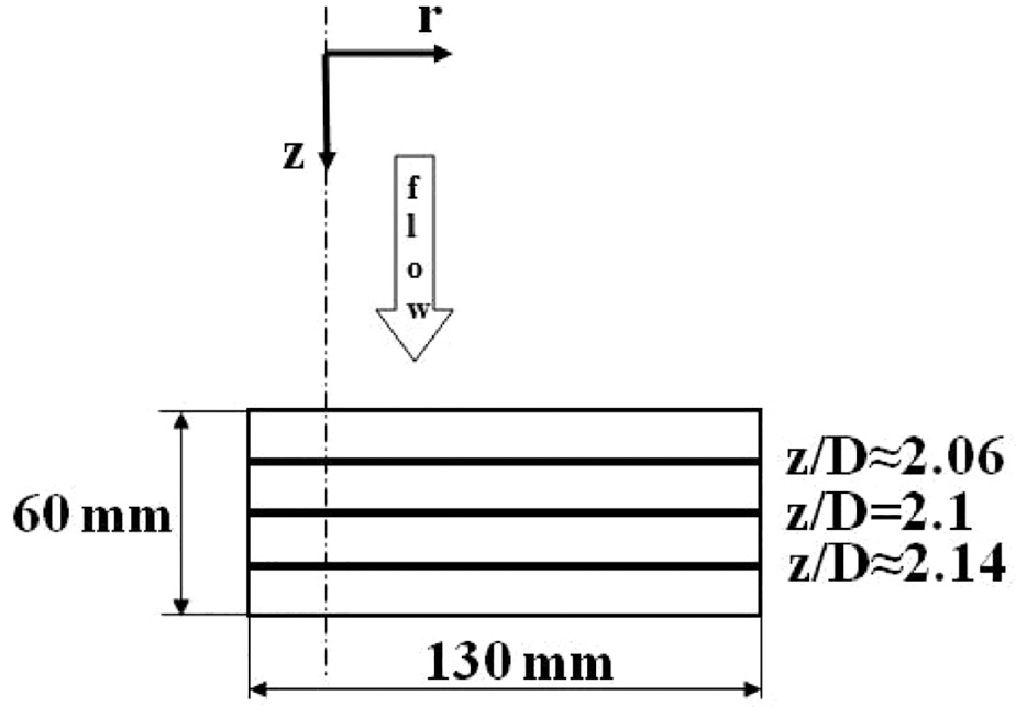
This straight pipe has total length of 20D, where the pipe inner diameter is D = 2R ≈ 0.402 m. It is followed by the exhaust hose, Venturi flow meter, regulation valve, and booster fan. Software coordinate system is presented in Figure 2.

Figure 2.

Measurement cross-section in position z/D = 2.1, with the coordinate system: 1 and 2 – left and right, respectively, high speed cameras FASTCAM SA4, by Photron, 3 – coordinate system in the measuring section, 4 – axial fan impeller, and 5 – profiled inlet.

Measuring sections are presented in Figure 3, where 1 – Nd:YLF laser, 2 and 3 – high speed cameras, 4 – axial fan impeller, and 5 – profiled inlet.

Figure 3.

Measurement planes, with the coordinate system: (a) cross-section (x-y plane) and (b) meridian section (z-x plane).

HSS PIV measurements and parameters for data analysis are provided in Mattern et al. ⁴ and Čantrak et al. ¹⁰ A dual oscillator-single head, diode pumped Nd:YLF laser Darwin Duo, by Quantronix, with an output light wavelength of 527 nm was used for flow illumination. Two high speed cameras FASTCAM SA4 by Photron, with scheimpflug tilt adapters and two Canon EF 85 mm f/1.8 USM lenses on automated EOS Rings from ILA GmbH were employed in the experiments. Photron FASTCAM Viewer software was used for recording. Resolution was 1008 × 1024 pix at 4000 fps. The time delay between two laser pulses was 50 μs. So, every single PIV vector field is averaged over this time interval. The flow was seeded by the Antari Z3000 fog machine with the Eurolite Smoke Fluid “-X-Extrem A2.” Seeding was naturally sucked in the test rig by the axial fan impeller, so the particle were well scattered in the flow. The post processing was performed by the software PIVview Version 3.2. Cylindrical pipe was a challenge for measurements, so common methods of dewarping and disparity correction were applied. The integration area for cross correlation was 32 × 32 pix and the overlap was 50%. ⁴ The distributions of the time-averaged velocity fields are calculated based on 2771 correlations.

Thorough analysis of the velocity measuring uncertainty on the same test rig is presented in Mattern et al. ¹⁵ Namely, PIV measurements have been compared in some points in the velocity field with the LDA (laser Doppler velocimetry) measurements. This analysis showed a clear and good correlation in time and magnitude between the performed time-resolved PIV and LDA signals. It was shown that the systematic error is in the range of approximately 0.5 m/s and it is independent of flow velocity and turbulence intensity. This could be even improved by fine-tuning of the PIV system.

Fan characteristic curve is tested and reported in Mattern et al. ⁴

Integral flow parameters

Radial distributions of the non-dimensional time averaged axial (U), radial (V), circumferential velocities (W), as well as circulation (rW) are shown in Figure 4 for the measuring cross-section (x-y plane), as well as meridian section (z-x plane) for z/D = 2.1, along θ = 0°. Diagrams with the abbreviation “mer” denote results from the meridian plane. The distributions of the time-averaged velocity fields are calculated as the average of 2771 PIV correlations. All velocities correspond to a cylindrical coordinate system and were made non dimensional by the averaged value of the axial velocity U_m = 6.85 m/s. Reynolds number is Re = 176,529. Volume flow rate is Q = 0.8695 m³/s. Calculated circulation is Г = 7.98 m²/s. Swirl number, that is one of the characteristics for the turbomachinery, is Ω = Q/(RГ) = 0.542, while flow rate coefficient is φ = 0.271.

Figure 4.

Radial distributions of the non-dimensional, time-averaged velocities, and circulation in the measuring cross-section (x-y plane), as well as the meridian section (z-x plane) in z/D = 2.1, along θ = 0°.

Profiles of all three average velocities in the cross and meridian sections are almost totally overlapped (Figure 4). Presented profile of the circumferential velocity presents Rankine swirl, which is composed of the forced vortex in the central region, also named as a “solid body,” and free vortex in the outer region, also named as a “sound flow region.” It could be also seen that as circumferential velocity profile reaches the value of zero on the pipe axis, and afterwards increases, that it is symmetrical. This shows that the axially restricted turbulent swirling flows are more stable than the unrestricted ones. ⁸

Circumferential velocity linear distribution characterizes the solid body region in the vortex core. Shear layer, which is between the vortex and outer region, is characterized by W_max (Figure 4). This value is reached in the position r/R = 0.325. Outer region, also named as a “sound region,” is characterized hereby almost constant circulation (rW ≈ const.). The fourth region is the boundary layer, that is wall region. It is here of great interest that this region is captured by using the HSS PIV system.

Axial velocity distribution reveals back flow region in the vortex core and almost constant distribution in the sound flow region.

Radial velocity is very small and approximately zero in the sound flow region, while in the vortex core region it increases and reaches maximum (V/U_m)_max = 0.3 at the pipe axis.

Figure 5(a) presents instantaneous total velocity field measured in the cross-section (x-y plane), while Figure 5(b) presents instantaneous total velocity field measured in the meridian section (z-x plane).

Figure 5.

Instantaneous total velocity field ( $\tilde{\mathrm{c}}$ ) measured in the (a) cross-section (x-y plane) and (b) meridian section (z-x plane).

It is obvious that instantaneous velocity fields, although not taken at the same moment, almost overlap. This is also shown after the comparison between the average total velocity fields in paper ¹⁰ for very close flow parameters. Figure 6 shows the average total velocity field (c) in the z-x plane.

Figure 6.

Average total velocity field (c) in the meridian section (z-x plane).

It shows that the velocity is symmetrical, as also presented in Figure 4 for the plane z/D = 2.1

Reynolds stresses and statistical moments

Distribution of turbulence levels is shown in Figure 7. Turbulence levels reach local maxima, for all velocities, in the vortex core region. After this, turbulence level decreases and increases again in the shear layer region.

Figure 7.

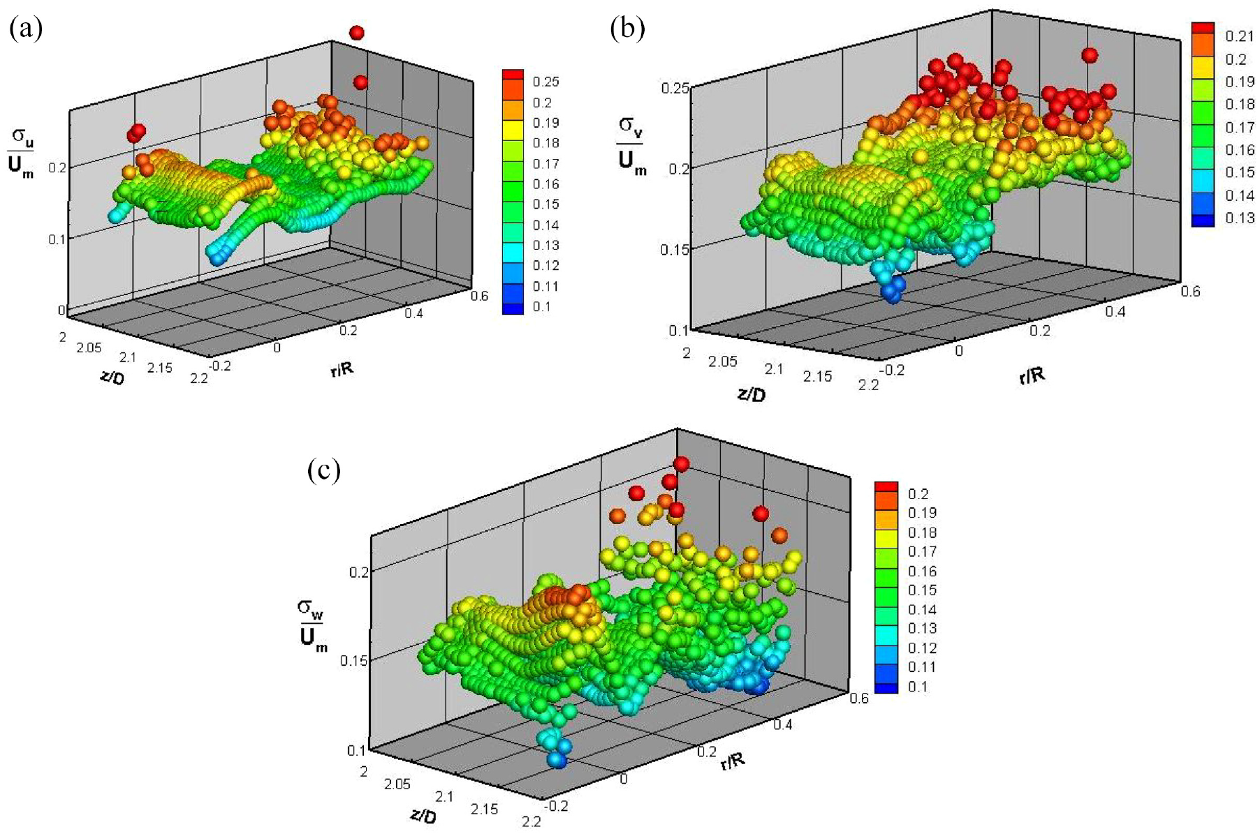
Turbulence levels in the meridian section (z-x plane) for: (a) axial, (b) radial, and (c) circumferential velocities.

Figure 8 shows turbulence level distributions for all three velocities measured in the meridian z-x plane in the measuring section z/D = 2.1, along the θ = 0° direction.

Figure 8.

Turbulence levels for all three velocities in position z/D = 2.1, along direction θ = 0°, in the meridian section (z-x plane).

The highest levels of turbulence are reached in almost all regions for the radial velocity, while the minima are reached in almost all points for the circumferential fluctuating velocity. It is also obvious that the maxima reached on the pipe axis are almost identical for all three velocity components. This indicates turbulence isotropy on the pipe axis. This will be also discussed with the help of the invariant maps (Figure 12(b)).

Radial and circumferential velocities have very similar trend in the vortex core region, decreasing in the region closest to the pipe axis, for r/R =  (0, 0.1), and afterwards increasing till r/R = 0.16. Both distributions reach their local minima in the point r/R = 0.1. All three distributions show different behavior in the vicinity of the shear layer region, characterized by W_max in position r/R = 0.325. Turbulence level for radial velocity is the highest and constant, while for circumferential velocity it decreases and, at the end, increases for axial velocity. Although stochastic, all three velocities have similar behavior in the sound flow region. Turbulence level for circumferential velocity reaches here its global minimum.

Statistical moments of the third (skewness factor S) and the fourth (flatness factor F) order are determined as follows:

$${\mathrm{S}}_{\mathrm{i}}=\overline{{\mathrm{u}}_{\mathrm{i}}^3}/{\sigma }_{\mathrm{i}}^3,{\mathrm{F}}_{\mathrm{i}}=\overline{{\mathrm{u}}_{\mathrm{i}}^4}/{\sigma }_{\mathrm{i}}^4,$$

(1)

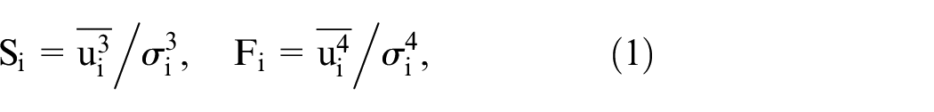
where i = u, v, w, and σ_i is standard deviation. Skewness and flatness factors are presented in Figure 9.

Figure 9.

Skewness factors in the meridian section (z-x plane) for (a) axial, (b) radial, (c) circumferential velocities, and (d) flatness factor in the meridian plane (z-x) for axial velocity.

It can be seen like in all results presented above that distributions are symmetrical to the pipe axis. It is obvious that all skewness and flatness factors differ from the values for normal, that is Gaussian distribution, which are zero and three, respectively. Skewness factor distributions are very similar to all three velocities. However, the closest values to those for normal distribution are reached for the axial velocity, that is S_u (Figure 9(a)) in almost all measuring points. This is followed by the radial (Figure 9(b)), and the most extreme values are reached for the circumferential velocity (Figure 9(c)). The extreme values in all three cases are reached, like in the case of the turbulence levels, in the vicinity of the shear layer region. Negative skewness factors, which exist in all three cases, indicate that large velocity fluctuations are negative (Figure 9(a)–(c)).

The values of flatness factor for axial velocity (F_u) have values higher than 3 (Figure 9(d)) in the vicinity of the pipe axis. This indicates great probability of small fluctuations.

The following figures present averaged Reynolds shear stresses calculated on the basis of the HSS PIV results measured in the meridian (z-x) plane (Figure 10).

Figure 10.

Non-dimensional Reynolds shear stress determined in the meridian section (z-x plane).

All Reynolds shear stresses have characteristic distributions for turbulent swirl flow. This opens discussion on the non-gradient turbulent transfer in swirl flows, what is also discussed in Čantrak et al. ¹⁶

Presented results in this chapter reveal all possibilities of application of the HSS PIV velocity data. The following chapter will present a research on the turbulence structure using the invariant maps, which are calculated after the Reynolds stresses.

Application of invariant maps derived from the HSS PIV data

The idea underlying turbulence investigation is a quantitative description of turbulence anisotropy. The approach of calculation of the invariant (Lumley) maps presented here is based on the HSS PIV data.

Anisotropy tensor is introduced as the measure of anisotropy, ¹⁷ where its components are a_ij. Three independent invariants are expressed as:

$$\begin{array}{c}\multicolumn{1}{c}{{\mathrm{I}}_{\mathrm{a}}=0,\mathrm{I}{\mathrm{I}}_{\mathrm{a}}=-\frac{1}{2}{\mathrm{a}}_{\mathrm{ij}}{\mathrm{a}}_{\mathrm{ji}},\mathrm{II}{\mathrm{I}}_{\mathrm{a}}=\frac{1}{3}{\mathrm{a}}_{\mathrm{ij}}{\mathrm{a}}_{\mathrm{ik}}{\mathrm{a}}_{\mathrm{jk}},\mathrm{where}{\mathrm{a}}_{\mathrm{ij}}}\\ =\frac{1}{2\mathrm{k}}\overline{{\mathrm{u}}_{\mathrm{i}}{\mathrm{u}}_{\mathrm{j}}}-\frac{1}{3}{\delta }_{\mathrm{ij}}\mathrm{and}\mathrm{k}=\frac{1}{2}(\overline{{\mathrm{u}}^2}+\overline{{\mathrm{v}}^2}+\overline{{\mathrm{w}}^2}),\hfill \end{array}$$

(2)

where k is turbulence kinetic energy and δ_ij is Kronecker delta.

Positions of the calculated invariant maps in the meridian section (z-x plane) are given in Figure 11.

Figure 11.

Positions of the calculated invariant maps in the meridian section (z-x plane).

Calculated invariant maps are presented in the following figures. Figure 12(a) shows characteristic points with their coordinates, where 0 (0, 0) denotes three-component isotropic turbulence, 1 (2/27, 1/3) one-component isotropic turbulence, and 2 (−1/108, 1/12) two-component isotropic turbulence. Boundaries of the invariant maps are given as follows:

$$\overline{21}:-\mathrm{I}{\mathrm{I}}_{\mathrm{a}}=3\mathrm{II}{\mathrm{I}}_{\mathrm{a}}+\frac{1}{9};201:-\mathrm{I}{\mathrm{I}}_{\mathrm{a}}=\frac{3}{4}{\left(4\left|\mathrm{II}{\mathrm{I}}_{\mathrm{a}}\right|\right)}^{2/3}.$$

(3)

Figure 12.

Invariant maps: (a) whole meridian section (z-x plane) and (b) along the pipe axis.

Straight line $\overline{21}$ presents cases of two-component turbulence, while 20 presents axis-symmetric turbulence (contraction) and 01 axis-symmetric turbulence (expansion).

All points from the meridian section (z-x plane) are given in Figure 12(a). Almost all points are positioned in the area between the 20 and 01 boundaries in the vicinity of the state of three-component isotropic turbulence (0). Now, the focus is here on the points on the pipe-axis.

Three-component isotropic turbulence (state 0) is reached on the pipe axis (Figure 12(b)) and remains in that point for all measurement positions along pipe axis in the meridian section. This is also shown in Figure 8 and discussed in that chapter.

Invariant maps calculated in the sections denoted in Figure 12 are shown in the figures to follow. They all behave in a very similar manner. Some measuring points reach regions of the axis-symmetric turbulence contraction and expansion and they are in the vicinity of the point 0, which represents again the three-component isotropic turbulence (Figure 13).

Figure 13.

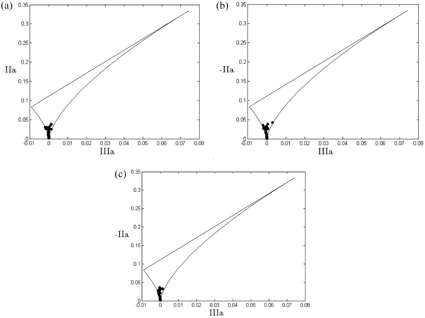
Invariant maps in the measuring sections z/D: (a) 2.06, (b) 2.1, and (c) 2.14.

Conclusions

HSS PIV experimental results obtained in this paper show the complexity of the turbulent swirl flow, axially restricted, generated by the axial fan in a pipe, as well as its three-dimensionality and non-homogeneity.

It could be concluded the following:

• Good overlapping of average velocity profiles is obtained using the HSS PIV in the meridian and pipe cross-section, although they are not measured at the same time. This is a consequence of the good experiment organization, as well as flow quasi-stationarity.

• Significance of the application of laser techniques such as HSS PIV, especially in the regions of recirculating flows – existence of the finite values of radial velocities in the vortex core, which again indicates that flow in the vortex core region must be studied as three-dimensional.

• Possibility to fast calculate relevant statistical characteristics of turbulence from HSS PIV.

• Determined invariant maps revealed three-component isotropic turbulence in the vortex core region, especially in the pipe axis and its zone. This is not case for the unrestricted flows, as shown in Čantrak et al. ⁹ On the basis of obtained invariant maps, Reynolds stresses (an)isotropy were found to manifest in a similar way even in different flow regions.

It can be concluded that fast measurement technique HSS PIV with invariant maps can rapidly resolve the nature of turbulence anisotropy in very complex flows such as the turbulent swirl flow. In addition, these experimental data, with the high turbulence levels, could be of great importance for CFD models calibration.