Sage Journals: Discover world-class research

Abstract

Integrated electro-mechanical actuators (EMAs) are widely used in cooperative robots. Their control system has to be carefully designed to achieve a desirable performance. The proportional-integral (PI) control and the active disturbance rejection control (ADRC) are the two commonly used controllers. Compared with the PI, the ADRC shows better performance in terms of disturbance rejection, response speed and overshooting suppression. However, the ADRC utilises numerous parameters and the optimisation of these parameters is a challenge. In this study, the influence of the parameters of β₀₁, β₀₂, β₀₃, β₁, β₂ on the ADRC performance is deeply analysed. Considering the two non-linear factors of permanent magnet synchronous motor and harmonic transmission in the EMA, a simulation model of the EMA was established. An improved swarm optimisation algorithm was employed to optimise the parameters of the ADRC. A second-order ADRC in speed and position modes was designed. The parameters of the ADRC in these modes were adjusted using improved particle swarm optimisation. ADRC was applied to the EMA field-oriented control system instead of cascade PI, and the simulation and experimental results were compared using the cascade PI control method. When the target speed is to 15 rpm, the speed fluctuation range of the ADRC is about ±0.3 rpm, which is smaller than that of the PI controller’s ±0.5 rpm. Compared with the cascade PI control, ADRC affords a faster response speed, greater robustness and stronger disturbance resistance in the steady-state operation process.

Keywords

Electro-mechanical actuator permanent magnet synchronous motor active disturbance rejection control simulation particle swarm optimisation field-oriented control

Introduction

Electro-mechanical actuators (EMAs) comprises a motor, a mechanical transmission and a driver. EMAs are widely used in robots, automobiles, navigation systems, aviation, aeronautics, surgical systems and precision machine tools to name a few.^1–5 During the operation of the EMA, a series of actions are intermittently and frequently performed. An EMA is required to output a large torque in a limited space and realise accurate speed and positional control. EMAs are mainly integrated with a permanent magnet synchronous motor (PMSM) or a brushless direct current (BLDC) motor, precision harmonic reducers, drives, controllers and other devices. EMAs are generally compact, lightweight, capable of accurate positioning and afford a large output torque. PMSM has the advantages of simple structure, small volume, light weight, high efficiency and fast response. Currently, PMSM control methods mainly include PI,⁶ intelligent control,^7–9 PID hybrid intelligent control mode, sliding mode variable structure control^10,11 and active disturbance rejection controller (ADRC).^12–16 The cascade PI control method is most commonly used in PMSM control systems, where the current loop is the inner loop, the velocity loop is the middle loop and the position loop is the outer loop.^17,18 This control method has the advantages of a simple structure, easy implementation and convenient adjustment of the control parameters. However, the PI controller has some disadvantages such as tracking delay, susceptibility to interference and an inability to compromise between overshoot and speed.^19,20 During operation of the EMA operation, start–stop and speed regulation functions must be frequently performed. If overshoot and oscillation occur during the process of start-up and speed regulation, long-term operation will cause precision harmonic reducer to exhibit a certain wear and reduce the accuracy of the EMA. When the structural parameters of the controlled system are known and fixed, stable control can be achieved using PI. However, the EMA is a complex time-varying non-linear system and the introduction of a harmonic reducer greatly enhances the non-linear factors of the system. In the actual operation process, the resistance, inductance and flux linkage change with the temperature, thereby reducing the accuracy and robustness of PI control.

It is difficult to achieve high-precision control of EMAs using a PI controller. Han proposed an ADRC theory based on an in-depth analysis of PID control.¹² This theory does not depend on precise mathematical modelling of the controlled object. An ADRC sets the system in the form of an integral series and achieves high-precision. control performance through the real-time estimation of internal and external disturbances and the compensation of control signals.²¹ ADRCs have been widely used in the field of motor control. In previous reports,^22,23 the physical meaning of ADRC was investigated and the second-order ADRC was applied to the position servo system. Prior studies²⁴ proposed a position current double-loop control method based on ADRC, which improved the disturbance rejection ability of the servo system. The model compensation method was applied to the second-order ADRC system, which effectively enhanced the observation accuracy of the extended state observer (ESO) and the tracking accuracy of PMSM.¹⁶ Fuzzy ADRC was used to replace the PI controller to realise position control.²⁵ Previously,^26,27 the first-order ADRC was used for the current loop, the second-order ADRC was used for the position loop. It was verified that this control method has the advantages of high tracking speed and non-overshoot performance. The second-order ADRC was used in prior studies^28,29 to improve the disturbance resistance and control accuracy of the PMSM position control process. Moreover, ADRCs have been used to study interior PMSM control and applied for sensorless control.^27,30,31

The ADRC has numerous parameters and requires tedious tuning. ADRC parameter tuning methods mainly include empirical methods, bandwidth/zero pole assignment methods, neural network and the swarm intelligence algorithm. The parameters that need to be adjusted for the second-order ADRC are $β_{01}$ , $β_{02}$ and $β_{03}$ in ESO and $β_{1}$ and $β_{2}$ in non-linear states error feedback (NLSEF). The EMA utilises the PMSM and harmonic reducer, which significantly increase the non-linear factors of the system. The PMSM and harmonic reducer are two major non-linear factors that pose a significant challenge for the construction of a mathematical model of the EMA system.

The traditional method of tuning system control parameters has significant limitations. The two non-linear factors are regarded as a combined factor. Based on the PMSM field-oriented control (FOC) model, the harmonic gear drive module was added to PMSM output and the EMA simulation model was established using MATLAB/Simulink. The inertia weight of sigmoid variation law and the learning factor of linear variation law has been used to improve the standard particle swarm optimisation (PSO). Using the improved PSO (IPSO) for multi-space optimisation, the control parameters required by the system can be obtained quickly and accurately. By changing the input and control parameters of the ADRC, position control and speed control can be realised.

In this study, the IPSO method was introduced to adjust the parameters of ADRC in an EMA control system for better control conformance. A second-order ADRC for position and speed modes is proposed to realise position and speed control. The feasibility of the control method is verified via simulation and experiment and compared with the PI controller. The results show that the control method can realise speed/position mode operation and lead to fast response, non-overshoot and strong disturbance resistance.

Mathematical model of PMSM for EMA

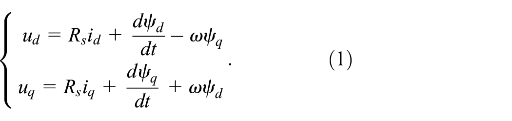
The mathematical model of the PMSM for the EMA comprises the voltage, flux, torque and mechanical equations. To simplify the analysis and not affecting the control, the saturation of the motor core, eddy current loss and hysteresis loss are ignored. The stator winding current is a three-phase symmetrical sinusoidal current. Under the FOC method, in the d–q coordinate system, the voltage equation is provided as follows:

{\begin{matrix} u_{d} = R_{s} i_{d} + \frac{d ψ_{d}}{d t} - ω ψ_{q} \\ u_{q} = R_{s} i_{q} + \frac{d ψ_{q}}{d t} + ω ψ_{d} \end{matrix} .

(1)

The flux equation for d–q axis is

{\begin{matrix} ψ_{d} = L_{d} i_{d} + ψ_{f} \\ ψ_{q} = L_{q} i_{q} \end{matrix} .

(2)

The electromagnetic torque equation is

T_{e} = 1.5 p_{n} [ψ_{f} i_{q} + (L_{d} - L_{q}) i_{d} i_{q}] .

(3)

The mechanical equation is

J \frac{d ω_{r}}{dt} = T_{e} - T_{L} - B ω_{r} .

(4)

Where R_s is the winding resistance and i_d, i_q, u_d, u_q, L_d, L_q, ψ_d and ψ_q are the d–q axis current (i), voltage (u), inductance (L) and flux linkage (ψ), respectively. p_n is the polar logarithm, T_e is the electromagnetic torque, J is the moment of inertia, T_L is the load torque, B is the damping coefficient. ψ_f is the permanent magnet flux linkage, ω is the electrical angular velocity and ω_r is the mechanical angular velocity. For a surface-mounted PMSM, L_d = L_q = L_s . When L_d = L_q = L_s or i_d = 0, equation (3) can be simplified as

T_{e} = 1.5 p_{n} ψ_{f} i_{q} .

(5)

ADRC control principle and parameter tuning

Mathematical model of ADRC

ADRC is a non-linear control method that does not require an accurate mathematical model of the controlled object. It can make real-time estimation and compensation for the internal and external disturbances of the system and achieve excellent control performance through non-linear feedback.³² An ADRC includes a tracking differentiator (TD), an ESO and an NLSEF. The transition process arranged by the TD can eliminate the compromise between overshoot and speed as well as realise fast target tracking without overshoot. ESO is the core component of an ADRC. It can effectively observe the system output and internal and external disturbances and extract the interference signal from the controlled output. The compensation in the control law can effectively improve the disturbance resistance of the system. NLSEF involves a non-linear combination of the TD and ESO output. Simultaneously, the output of NLSEF and the ‘total disturbance’ estimator of ESO are coupled to perform on the controlled plant.

The expression of the differential equation for an uncertain object subjected to unknown disturbance is given as follows:

{\begin{matrix} x^{n} = f (x, \overset{\cdot}{x}, ~, x^{(n - 1)}, t) + d (t) + bu (t) \\ y = x (t) \end{matrix} .

(6)

Here, $f (x, \overset{\cdot}{x}, ~, x^{(n - 1)}, t)$ is an unknown function, $d (t)$ is an unknown disturbance, y is the system output and $u (t)$ is the system control quantity. The block diagram showing the principle of the ADRC structure is presented in Figure 1.^33,34

Figure 1.

Schematic diagram of an Active disturbance rejection control (ADRC) structure.

First- and second-order ADRC are generally used in practical application. The third-order ADRC has a complex expression and needs a long calculation time, which requires a high-performance controller; it is thus rarely used in practice. The second-order ADRC equations are represented by equations (7)–(9).

For TD,

{\begin{matrix} x_{1} (k + 1) = x_{1} (k) + T x_{2} (k) \\ x_{2} (k + 1) = x_{2} (k) + Tfhan (x_{1} (k) - x^{*}, x_{2} (k), r, h_{1}) \end{matrix} .

(7)

Here, x* is the input signal, $x_{1}$ is the tracking signal of x*, $x_{2}$ is the differential of x₁, r is the speed factor, which determines the tracking speed, T is the sampling time and h₁ is the filter factor; fhan(.) is the fastest synthesis function, expressed as follows:

{\begin{matrix} d = r h_{1}; d_{0} = h_{1} d \\ y = x_{1} + h_{1} x_{2} - v (k); a_{0} = \sqrt{d^{2} + 8 r | y |} \\ a = {\begin{matrix} x_{2} + \frac{(a_{0} - d)}{2}, | y | > d_{0} \\ x_{2} + \frac{y}{h_{1}}, | y | \leq d_{0} \end{matrix} \\ fst = {\begin{matrix} - \frac{ra}{d}, | a | \leq d \\ - rsign (a), | a | > d \end{matrix} \end{matrix} .

(8)

For ESO,

{\begin{matrix} e (k) = z_{1} (k) - y (k) \\ z_{1} (k + 1) = z_{1} (k) + T (z_{2} (k) - β_{01} e) \\ z_{2} (k + 1) = z_{2} (k) + \\ T (z_{3} (k) - β_{02} fal (e (k), α_{01}, δ) + b_{0} u (k)) \\ z_{3} (k + 1) = z_{3} (k) - T β_{03} fal (e (k), α_{02}, δ) \end{matrix} .

(9)

Here, e(k) is the error signal, $y (k)$ is the output of the system, $z_{1} (k)$ is the tracking signal of $y (k)$ , $z_{2} (k)$ is the tracking signal of $z_{1} (k)$ and $z_{3} (k)$ is the total disturbance of the system. $z_{3} (k)$ is fed back to the control quantity to realise compensation. b is the compensation factor. β₀₁, β₀₂ and $β_{03}$ are output error correction gains. α₀₁ and α₀₂ are the non-linear factors. $δ$ is the filter factor. If fal(·) is a non-linear function, it is called a non-linear ESO. If fal(·) = e, it is called the linear ESO.

For NLSEF,

{\begin{matrix} e_{1} (k) = x_{1} (k) - z_{1} (k) \\ e_{2} (k) = x_{2} (k) - z_{2} (k) \\ u_{0} (k) = β_{1} fal (e_{1} (k), α_{1}, δ) + β_{2} fal (e_{2} (k), α_{2}, δ) \\ u (k) = u_{0} (k) - \frac{z_{3} (k)}{b_{0}} \end{matrix} .

(10)

Here, $e_{1} (k)$ and $e_{2} (k)$ are error signals and $β_{1}$ and $β_{2}$ are the error and differential gains respectively. When 0 < α < 1, fal(.) realises the mathematical fitting of ‘small error large gain, large error small gain’. Variable gain PID, fuzzy control and intelligent control are all based on the control idea of ‘small error and large gain, large error and small gain’. fal(.) is a non-linear feedback function, specifically expressed as

fal = {\begin{matrix} {| e |}^{α} sgn (e), | e | > δ \\ \frac{e}{δ^{(1 - α)}}, | e | \leq δ \end{matrix} .

(11)

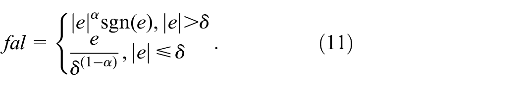
Figure 2(a) shows the change in $fal (e, α, δ)$ when $α$ is varied and $δ$ fixed, and Figure 2(b) shows the change in $fal (e, α, δ)$ when $δ$ is varied and $α$ is fixed.

Figure 2.

Changes in $fal (e, α, δ)$ function with different (a) α and (b) δ values. (a) δ = 0.5, different α values (b) α = 0.5,different δ values.

ADRC parameters tuning rules

The main parameters to be adjusted in the TD are the velocity factor (r) and the filter factor (h₁). The velocity factor mainly affects the tracking effect. A larger velocity factor corresponds to a shorter transition time and thus a faster tracking response. However, very large velocity factor leads to overshoot and oscillation. When the velocity factor is constant and the filter factor is large, the tracking signal error is large; when the h₁ is small, the noise suppression is more prominent. However, when the h₁ is too small, the ability of the TD to suppress noise will be weakened.

The role of the ESO is to observe and compensate for both internal and external disturbances, which is the core function of the ADRC. The disturbance compensation factor $b_{0}$ mainly affects the disturbance compensation capacity. If the system disturbance is significant, b₀ should be slightly larger; if the system disturbance is small, b₀ should be marginally lower.

Directional adjustment is adopted. When we set $α_{01} = α_{02}$ =1, $fal (e, α, δ)$ can be linearised to $fal (e, α, δ) = e$ . Then, equation (9) is rewritten as

{\begin{matrix} e (k) = z_{1} (k) - y (k) \\ z_{1} (k + 1) = z_{1} (k) + T (z_{2} (k) - β_{01} e) \\ z_{2} (k + 1) = z_{2} (k) + T (z_{3} (k) - β_{02} e + b_{0} u (k)) \\ z_{3} (k + 1) = z_{3} (k) - T β_{03} e \end{matrix} .

(12)

The characteristic expression of equation (12) is obtained using Laplace transformation:

p (s) = s^{3} + β_{01} s^{2} + β_{02} s + β_{03} .

(13)

According to the bandwidth-parameterisation-based controller tuning method proposed by Gao,³⁵ the reference value for the parameters β₀₁, β₀₂ and β₀₃ can be obtained as follows:

β_{01} = 3 ω_{c}, β_{02} = 3 {ω_{c}}^{2}, β_{03} = {ω_{c}}^{3} .

(14)

The values for the parameters β₀₁, β₀₂ and β₀₃ need to be adjusted in practical applications according to the system output. The tuning rules for these parameters are listed in Table 1. Notably, when one parameter is tuned, the other two remain constant.

Table 1.

Tuning rules for β₀₁, β₀₂ and β₀₃ parameters.

System response phenomena	Constantparameters	Tuning rules
Oscillation occurs	β₀₂, β₀₃	Decrease β₀₁
Divergence occurs		Decrease β₀₁
Steady-state high-frequencyoscillation occurs		Increase β₀₁
High-frequency oscillation occurs	β_01,β₀₃	Decrease β₀₂
Disturbance rejection performance decrease		Increase β₀₂
Oscillation amplitudeincrease		Increase β₀₂
Overshoot occurs		Increase β₀₂
Respond time is long	β_01, β₀₂	Increase β₀₃
Large oscillation occurs	β_01, β₀₂	Decrease β₀₃

The value of $δ$ in NLSEF is the same as that in ESO. $β_{1}$ and $β_{2}$ are equivalent to the proportional and differential coefficients of PID control, respectively. To achieve the ideal control effect, the parameters determined theoretically need to be adjusted for practical application.

Design of ADRC for PMSM

Second-order ADRC for position/speed compound controller

Rotational speed provides the differential signal of the rotor angle. The speed/position controller is designed as a second-order ADRC to replace the position and speed cascade PI controllers.

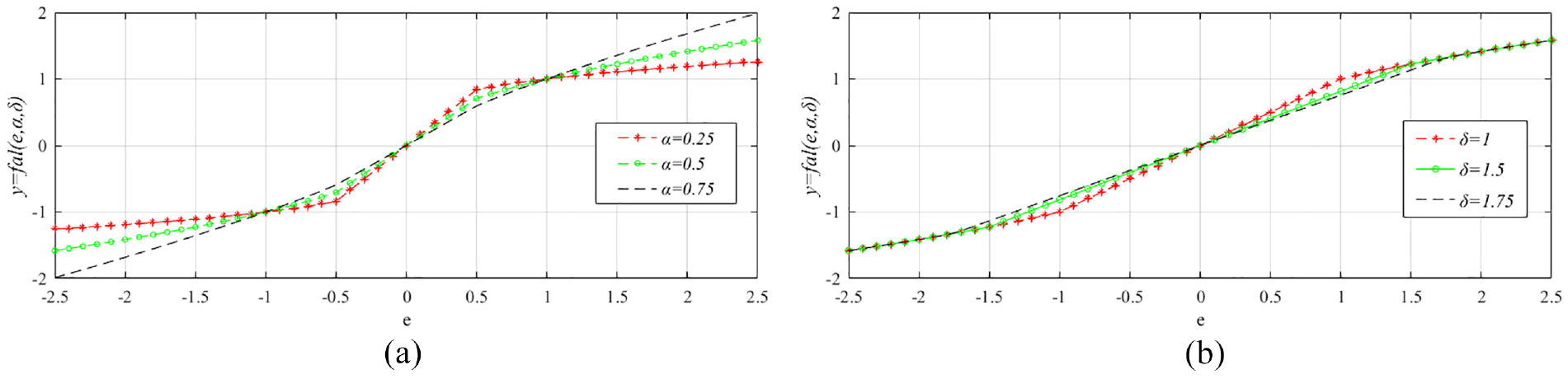
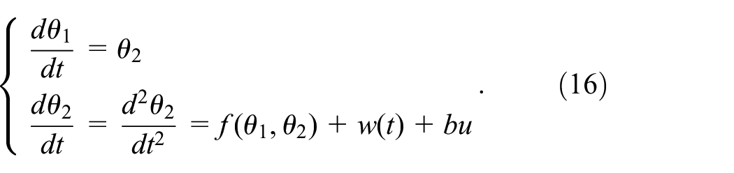
The second-order equation of state for the angle of the position loop is given as

\frac{d^{2} θ}{d t^{2}} = \frac{d ω_{r}}{dt} = 1.5 \frac{p_{n} ψ_{f}}{J} i_{q} - \frac{T_{L}}{J} - \frac{B ω_{r}}{J} .

(15)

Here, $θ$ is the rotor position, $ω_{r}$ is the rotor speed, $i_{q}$ is the control quantity, $- \frac{B ω_{r}}{J}$ is the known disturbance and $w (t) = - \frac{T_{L}}{J}$ , $b_{0} = 1.5 \frac{p_{n} ψ_{f}}{J}$ is the unknown disorder. The angle can be measured using the sensor. Thus, the second-order state equation of the position loop is given by

{\begin{matrix} \frac{d θ_{1}}{dt} = θ_{2} \\ \frac{d θ_{2}}{dt} = \frac{d^{2} θ_{2}}{d t^{2}} = f (θ_{1}, θ_{2}) + w (t) + bu \end{matrix} .

(16)

The fastest synthesis function fhan(.) can track the target position without overshoot. The displacement planning of TD is shown using equation (17).

{\begin{matrix} θ (k + 1) = θ (k) + T ω_{r} (k) \\ ω_{r} (k + 1) = ω_{r} (k) + T * fhan (θ (k) - θ_{ref}, ω_{r} (k), r_{0}, h) \end{matrix} .

(17)

Here, θ_ref is the target position. θ(k) and ω_r(k) are the angle and speed during operation, respectively. At steady state, $θ = θ_{ref}$ .

The process of moving the rotor to the target position involves load disturbance, change in the moment of inertia, etc. ESO can estimate and compensate for the position disturbance w(k) in real-time. The ESO of the second-order ADRC of the position ring is expressed as

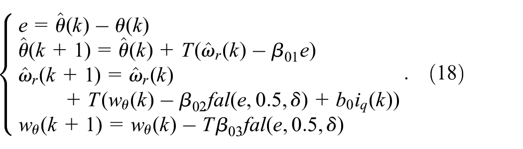
{\begin{matrix} e = \hat{θ} (k) - θ (k) \\ \hat{θ} (k + 1) = \hat{θ} (k) + T ({\hat{ω}}_{r} (k) - β_{01} e) \\ {\hat{ω}}_{r} (k + 1) = {\hat{ω}}_{r} (k) \\ + T (w_{θ} (k) - β_{02} fal (e, 0.5, δ) + b_{0} i_{q} (k)) \\ w_{θ} (k + 1) = w_{θ} (k) - T β_{03} fal (e, 0.5, δ) \end{matrix} .

(18)

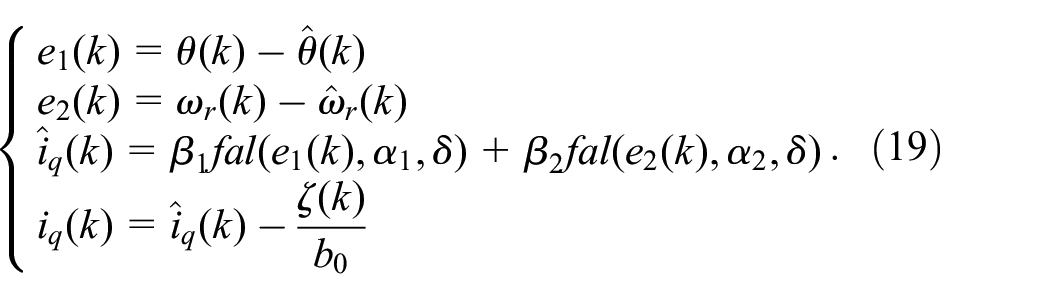
Here, $\hat{θ} (k)$ and $\hat{ω} (k)$ are estimators of $θ (k)$ and, $ω (k)$ respectively, and $w_{θ} (k)$ is the observed value of disturbance.

To improve the disturbance rejection ability of the controller, the non-linear control law is used herein. The non-linear control law of the position loop is designed as follows:

{\begin{matrix} e_{1} (k) = θ (k) - \hat{θ} (k) \\ e_{2} (k) = ω_{r} (k) - {\hat{ω}}_{r} (k) \\ {\hat{i}}_{q} (k) = β_{1} fal (e_{1} (k), α_{1}, δ) + β_{2} fal (e_{2} (k), α_{2}, δ) \\ i_{q} (k) = {\hat{i}}_{q} (k) - \frac{ζ (k)}{b_{0}} \end{matrix} .

(19)

Second-order ADRC for a speed loop

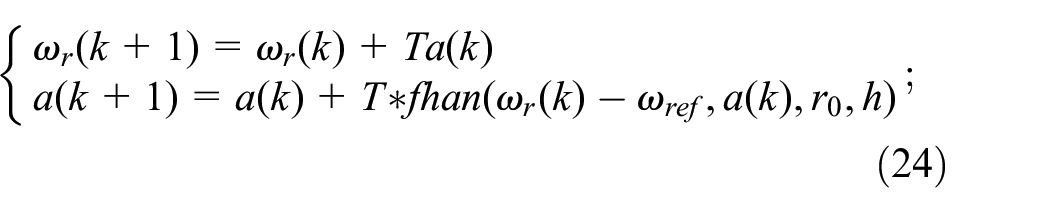
The target position entered in TD is changed to the target speed and the position signal fed back to the ESO is changed to the velocity signal. Second-order ADRC in speed mode can be realised by modifying the control parameters for second-order ADRC in the position mode.

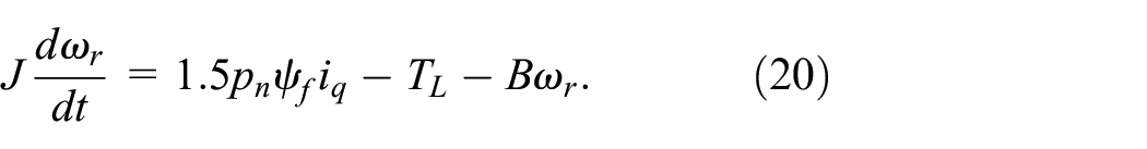
The state expression for the rotating speed is given by

J \frac{d ω_{r}}{dt} = 1.5 p_{n} ψ_{f} i_{q} - T_{L} - B ω_{r} .

(20)

By setting, $K_{1} = 1.5 p_{n} ψ_{f}$ and $T_{1} = T_{L} + B ω_{r}$ ,

J \frac{d ω}{dt} = K_{1} i_{q} - T_{1} .

(21)

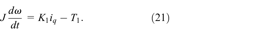
The differential of equation (21) leads to the following equation

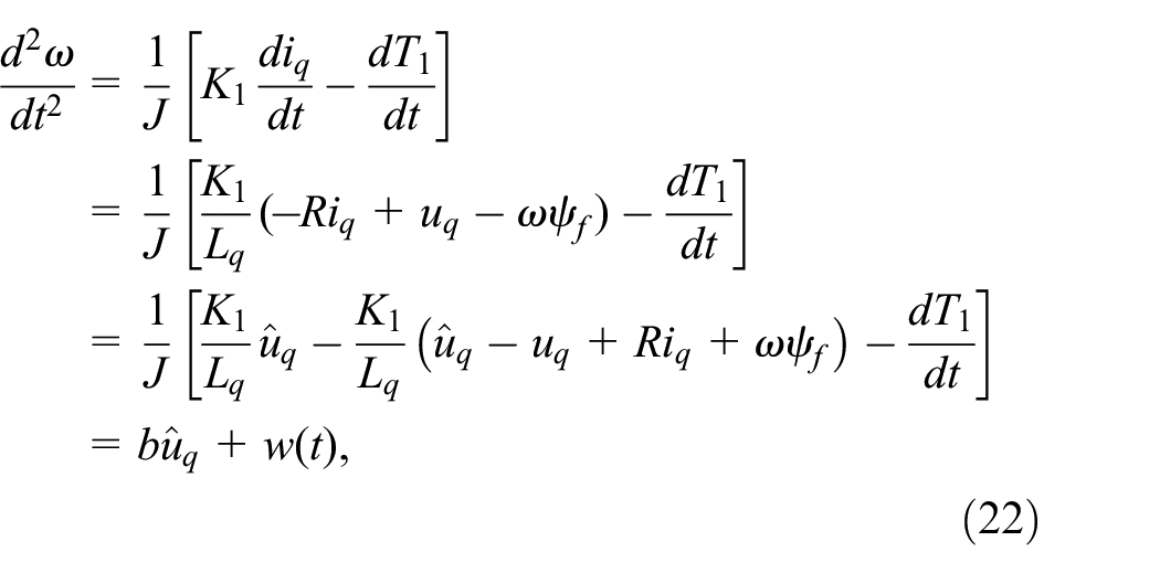
\begin{matrix} \frac{d^{2} ω}{d t^{2}} = \frac{1}{J} [K_{1} \frac{d i_{q}}{dt} - \frac{d T_{1}}{dt}] \\ = \frac{1}{J} [\frac{K_{1}}{L_{q}} (- R i_{q} + u_{q} - ω ψ_{f}) - \frac{d T_{1}}{dt}] \\ = \frac{1}{J} [\frac{K_{1}}{L_{q}} {\hat{u}}_{q} - \frac{K_{1}}{L_{q}} ({\hat{u}}_{q} - u_{q} + R i_{q} + ω ψ_{f}) - \frac{d T_{1}}{dt}] \\ = b {\hat{u}}_{q} + w (t), \end{matrix}

(22)

where $b = \frac{u_{dc} K_{1}}{\sqrt{3} J L_{q}}$ , $w (t)$ is the disturbance term, $w (t) = \frac{1}{J} [- \frac{K_{s}}{L_{q}} ({\hat{u}}_{q} - u_{q} + R i_{q} + ω ψ_{f}) - \frac{d T_{d}}{dt}]$ .

The structure of the second-order speed loop ADRC is the same as that of the second-order position/speed loop compound ADRC; however, the input variables of the controller are different. The input of the second-order speed ADRC is the set target speed and the actual feedback speed. The mechanical angular velocity is $ω_{r}$ , the state variable is ω_r1 and the angular acceleration is the state variable ω_r2. Thus, the following equation is obtained:

{\begin{matrix} \frac{d ω_{r 1}}{dt} = ω_{r 2} \\ \frac{d ω_{r 2}}{dt} = \frac{d^{2} ω_{r}}{d t^{2}} = f (ω_{r 1}, ω_{r 2}) + w (t) + b_{0} u \end{matrix},

(23)

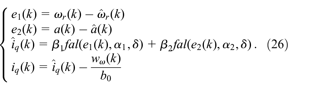
The second-order speed ADRC is presented using equation (24)–(26). The meaning of the parameters in the formulae is the same as for the position loop ADRC; $w_{ω} (k)$ is the observed value of disturbance, and $\hat{a} (k)$ is the acceleration observation.

{\begin{matrix} ω_{r} (k + 1) = ω_{r} (k) + Ta (k) \\ a (k + 1) = a (k) + T * fhan (ω_{r} (k) - ω_{ref}, a (k), r_{0}, h) \end{matrix};

(24)

{\begin{matrix} e = ω (k) - y (k) \\ {\hat{ω}}_{r} (k + 1) = {\hat{ω}}_{r} (k) + T (\hat{a} (k) - β_{01} e) \\ \hat{a} (k + 1) = \hat{a} (k) + T (w_{ω} (k) - β_{02} fal (e, 0.5, δ) + b_{0} i_{q} (k)) \\ w_{ω} (k + 1) = w_{ω} (k) - T β_{03} fal (e, 0.5, δ) \end{matrix};

(25)

{\begin{matrix} e_{1} (k) = ω_{r} (k) - {\hat{ω}}_{r} (k) \\ e_{2} (k) = a (k) - \hat{a} (k) \\ {\hat{i}}_{q} (k) = β_{1} fal (e_{1} (k), α_{1}, δ) + β_{2} fal (e_{2} (k), α_{2}, δ) \\ i_{q} (k) = {\hat{i}}_{q} (k) - \frac{w_{ω} (k)}{b_{0}} \end{matrix} .

(26)

A schematic of the second-order position mode and speed mode ADRC is shown in Figure 3. In the position mode, the ADRC inputs the target and current positions. In the speed mode, the ADRC inputs the target and current speeds.

Figure 3.

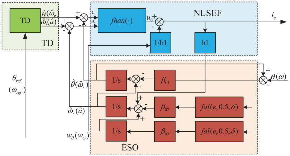
Schematic of second-order ADRC for determining EMA position and velocity.

In the abovementioned analysis, $β_{01}$ , $β_{02}$ and $β_{03}$ in ESO and $β_{1}$ and $β_{2}$ in NLSEF are the key factors affecting the controller. Two non-linear factors (PMSM and harmonic reducer) are integrated in EMA; thus, it is difficult to construct a mathematical model for the system. There are some limitations in tuning the control parameters of the system using traditional methods. In this study, the EMA model was built on the MATLAB/Simulink platform and the multi-objective parameters of the ADRC were adjusted using IPSO.

IPSO

PSO is derived from the study of foraging of birds. It was first proposed by Kennedy and Eberhart in 1995.³⁶ PSO has the advantages of a simple structure, fewer parameters, fast convergence speed and robust optimisation ability. It is applied to non-linear, multivariable and strong coupling control systems, which can search for the optimal global solution and achieve a good control effect.^37,38

In the D-dimensional search space, n particles are initialised to form a population. Each particle represents the potential optimal solution in the optimisation problem and its characteristics are represented by velocity, position and fitness. The position of the i-th particle in D-dimensional space is $X_{i} = (x_{i 1}, x_{i 2}, . . ., x_{iD})$ , $i = 1, 2, . . ., n$ . The velocity of the i-th particle is $V_{i} = (v_{i 1}, v_{i 2}, . . ., v_{iD})$ , $i = 1, 2, . . ., n$ . The individual extremum of the i-th particle searched for is $Pbes t_{i} = (p_{i 1}, p_{i 2}, . . ., p_{iD})$ , $i = 1, 2, . . ., n$ . The extremum of the population search for the group is $Gbes t_{i} = (g_{1}, g_{2}, . . ., g_{D})$ .

The velocity and position update formulae of the original PSO are as follows.

\begin{matrix} V_{id}^{k + 1} = V_{id}^{k} + c_{1} r and ({Pest}_{id}^{k} - X_{id}^{k}) \\ + c_{2} rand ({Gbest}_{d}^{k} - X_{id}^{k}) and \end{matrix}

(27)

X_{id}^{k + 1} = X_{id}^{k} + V_{id}^{k},

(28)

where $X_{id}^{k}$ is the D-dimensional component of the position vector for particle i in the k-th iteration, $d \in [1, D]$ . The range of the positional change is limited between V_min and V_max. ${Pest}_{id}^{k}$ represents the individual extremum of particle i in the D-dimensional component of the k-th iteration. ${Gbest}_{d}^{k}$ represents the population extremum of the k-th iteration population in the D-dimensional component. c₁ and c₂ are the learning factors, which mainly affect the target recognition ability for particles; rand is a random number between 0 and 1.

To address the issue of premature convergence encountered with the original PSO and the ease of falling into the optimal local solution, Shi³⁷ introduced the inertia weight factor of linear decline; thus, the speed update formula was transformed to

\begin{matrix} V_{id}^{k + 1} = ω V_{id}^{k} + c_{1} r and ({Pest}_{id}^{k} - X_{id}^{k}) \\ + c_{2} rand ({Gbest}_{d}^{k} - X_{id}^{k}) . \end{matrix}

(29)

The range of $ω$ for standard PSO is between 0.4 and 0.95 and the linear decreasing method is adopted; that is given as

ω = \frac{(ω_{max} - ω_{min}) (K_{max} - k)}{K_{max}} + ω_{min} .

(30)

Here, $ω$ is the inertia weight. $ω$ , c₁ and c₂ are the key factors affecting the convergence of PSO. When ω is large, the particle search range is wide and the global search ability is strong. When ω is small, the particle search range is narrow and the algorithm has strong local search ability. When c₁ is high, the behaviour of the particles is more independent, the convergence speed of the algorithm is slower and the blindness of the optimal global solution is more significant. When c₂ is large, the proportion of social cognition is greater, the consciousness of the particle group is stronger, the agglomeration phenomenon is more obvious and it is easier to obtain precocity. By changing the variation law of these three parameters, premature convergence of the PSO to fall into the optimal local solution can be avoided.

A reasonable search process must have robust global search ability in the early stage. With the evolution of PSO gradually narrowing the search area, the search process should have strong local search ability. ω and c₁ should be initially large and then small; c₂ should be initially small and then become large.

Based on this concept, the standard PSO is improved. The non-linear sigmoid function is used as the law of variation of $ω$ . By adjusting the coefficient of the sigmoid function, the value range is adjusted to [0.4, 0.95]. The non-linear decreasing mode of $ω$ is represented as follows:

ω = \frac{1}{1 + \exp [\frac{(\ln 1.5 + \ln 19) k}{K_{max}} - \ln 19]} .

(31)

c₁ and c₂ are no longer fixed values and vary linearly according to the number of iterations. The variation rules are as follows:

{\begin{matrix} c_{1} = {c_{1}}_{\min} + \frac{({c_{1}}_{max} - {c_{1}}_{min}) (K_{max} - k)}{K_{max}} \\ c_{2} = {c_{2}}_{\max} - \frac{({c_{2}}_{max} - {c_{2}}_{min}) (K_{max} - k)}{K_{max}} \end{matrix} .

(32)

To test the performance of the IPSO, the classical multimodal function Rastrigrin is used as the test object. The function has several local optimal solutions in the feasible region. The expression is given by

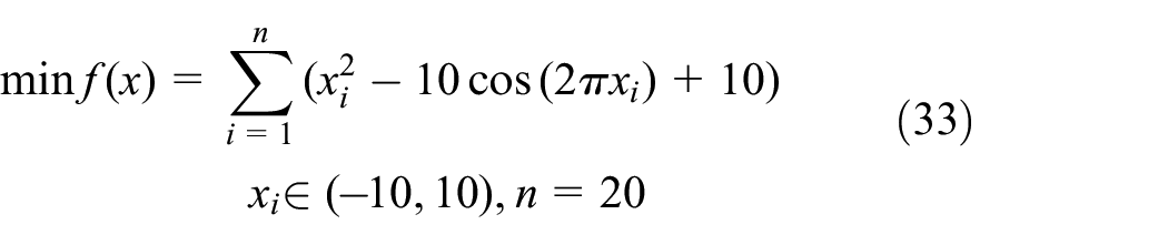
\begin{matrix} min f (x) = \sum_{i = 1}^{n} (x_{i}^{2} - 10 \cos (2 π x_{i}) + 10) \\ x_{i} \in (- 10, 10), n = 20 \end{matrix}

(33)

The minimum value of the function is 0 and the optimal position is (0, 0,…,0). Standard PSO, PSO based on sigmoid inertia weight (SPSO) and IPSO were used for the test. The population number and the number of iterations were set to 20 and 50, respectively. For standard PSO and SPSO, the learning factors were set as c₁ and c₂, with a value of 2. For IPSO, the learning factor was set to change between 0.1 and 2. The programme execution flow of IPSO is shown in Figure 4(a). The test results are shown in Figure 4(b).

Figure 4.

Flowchart of IPSO, and three algorithms test results: (a) Flowchart of IPSO and (b) comparison of convergence results of the three algorithms.

As shown in Figure 4(b), the three algorithms achieved the global extremum of 0. Standard PSO had the slowest convergence speed, followed by SPSO, whereas IPSO had the fastest convergence speed. IPSO has the advantages of good global convergence, fewer iteration times and high optimisation efficiency.

The common performance indexes of the control system are the integral of the squared error, integral of time multiplied by the squared error (ITSE), integral absolute error (IAE), integral of time multiplied by the absolute error (ITAE), etc. The details are as follows:

ISE = \int_{0}^{\infty} e^{2} (t) dt,

(34)

ITSE = \int_{0}^{\infty} t e^{2} (t) dt,

(35)

IAE = \int_{0}^{\infty} | e (t) | dt and

(36)

ITAE = \int_{0}^{\infty} t | e (t) | dt .

(37)

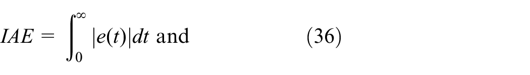
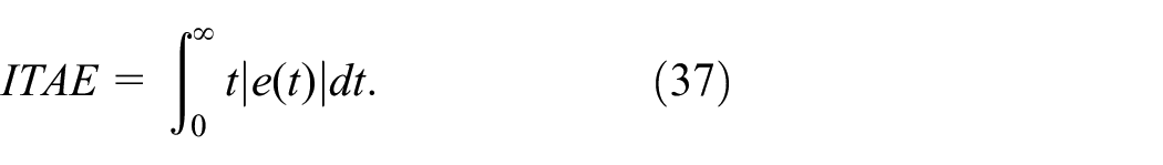
Equations (34) and (35) will cause a large overshoot to approach the target value in a short time. However, equations (36) and (37) considerably reduce this defect. IAE has good transient response characteristics. The disadvantage is that when the system parameters are different, the response on the performance index is not obvious. ITAE criterion can make the system have a fast transition process and high-precision steady-state tracking. The ITAE index has reasonable practicability and selectivity and has been widely used in single input–output and adaptive control systems.^39,40 In this study, ITAE was selected as the performance index function.

Simulation analysis and experimental verification

Simulation model

The block diagram of the EMA position and speed mode FOC based on the ADRC is shown in Figure 5. The control parameters for ESO and NLSEF in the ADRC were obtained using IPSO. Compared with the cascade PI control mode, the cascade PI controllers of the position and speed loops were integrated into the second-order ADRC speed/position composite controller. The stability and disturbance resistance ability of the system were improved via ESO disturbance compensation.

Figure 5.

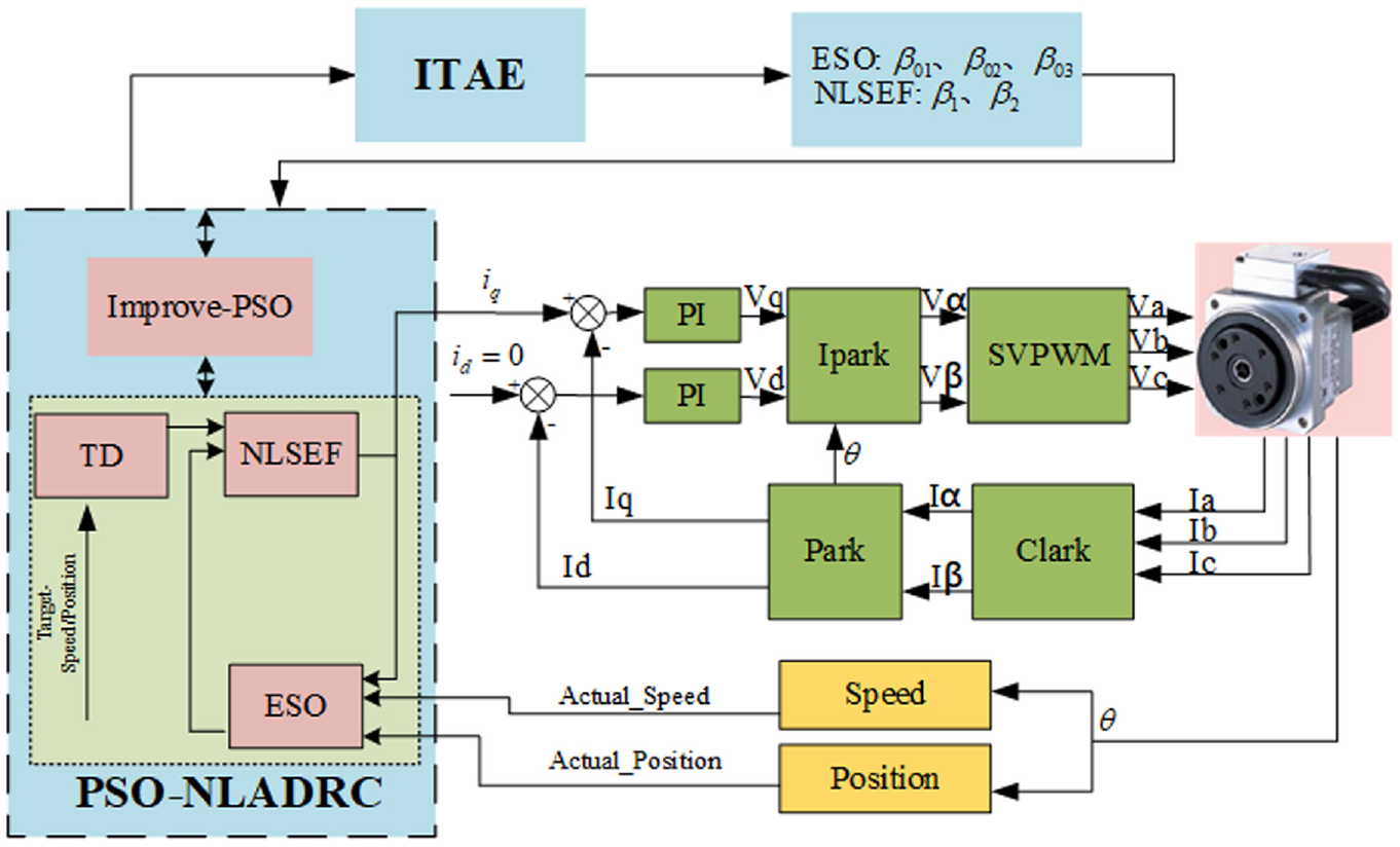
EMA position and speed compound controller based on IPSO.

The parameters to be set in the ADRC include $β_{01}$ , $β_{02}$ and $β_{03}$ in ESO and $β_{1}$ and $β_{2}$ in NLSEF. There are five parameters in total. ITAE is used as the fitness function of IPSO.

According to the modular design concept, the algorithm is divided into the ADRC module, ITAE, FOC control, PMSM and driver and harmonic reducer. The structure of Simulink for speed mode operation is shown in Figure 6. For position mode operation, only the input source of ADRC to the position signal needs to be changed.

Figure 6.

Simulink simulation models: (a) ADRC module, (b) ITAE module, (c) FOC calculation module, (d) PMSM and controller module and (e) Harmonic Driver Module.

Analysis of simulation results

The Simulink model utilises five parameters in the MATLAB workspace for simulation. The five parameters to be optimised in the ADRC were updated iteratively and the corresponding ITAE values were obtained. The population size was set to five and the number of iterations was limited to 20. Figure 7 presents a comparison of the iteration fitness of SPSO and IPSO over 20 iterations, demonstrating that the convergence speed and fitness value obtained using IPSO were better than those achieved using SPSO.

Figure 7.

Optimisation results for sigmoid PSO and improved IPSO.

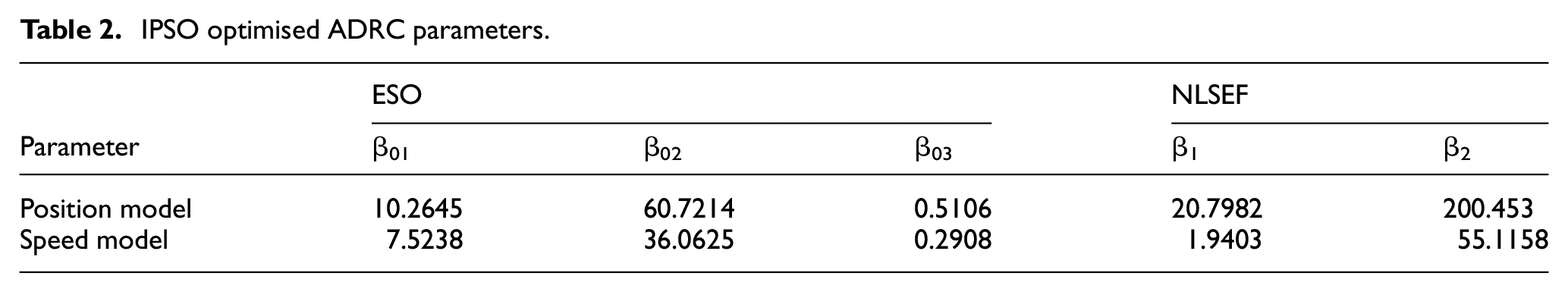
The control parameters for position and speed modes obtained using IPSO are summarised in Table 2.

Table 2.

IPSO optimised ADRC parameters.

	ESO			NLSEF
Parameter	β₀₁	β₀₂	β₀₃	β₁	β₂
Position model	10.2645	60.7214	0.5106	20.7982	200.453
Speed model	7.5238	36.0625	0.2908	1.9403	55.1158

The parameters for the current loop in cascade PI control mode were the same as those in the ADRC control mode. IPSO was used to optimise the parameters for the speed and position loops in cascade PI control mode. The population size was set to 2 and the number of iterations was set to 20. The obtained PI parameters for the speed and position loops are summarised in Table 3.

Table 3.

IPSO optimised PI parameters.

Parameter	P	I
Speed_LOOP	3.12	1.15
Position model_LOOP	175.2	0.2

Analysis of position simulation results

The input step signal and sine signal were used as follows to verify the stability of the cascade PI and ADRC modes. For step signal, the target position was set to 20 rad at the beginning, 50 rad at 0.5 s, 70 rad at 1 s, 50 rad at 1.5 s and 40 rad at 2 s. The simulation results are shown in Figure 8.

Figure 8.

Position control curve: (a) step signal response curve and (b) sinusoidal signal response curve.

Figure 8(a) demonstrates that the response speed for the ADRC is faster than that of the PI controller. The expanded region denoted as B shows that the PI control mode has a small overshoot, while regions A and C have no overshoot. For a set of fixed PI parameters, PI control cannot adapt to different target positions. In some control situations with high precision, it is often necessary to set multiple PI parameters in stages. As seen from the sinusoidal response curve in Figure 8(b), the sinusoidal tracking signal of the ADRC is faster than that of the PI controller. For some cases where the position frequency conversion is fast, using a set of fixed PI parameters lead to an ‘out-of-step’ situation.

Analysis of speed simulation results

The start-up target speed was set to 500 rpm. At 0.05 s, the target load was set to 1 N.m. The target speed was set to 1000 rpm at 0.1 s. The target load was set to 3 N.m at 0.15 s. The parameters of the PI controller and the ADRC were adjusted. The speed simulation results presented in Figure 9 show that the time required for the ADRC and PI controller to reach steady state is basically the same. However, PI control mode has noticeable overshoot before reaching steady state and tends to achieve the steady state after one oscillation, whereas the ADRC has no overshoot or oscillation.

Figure 9.

Speed simulation data.

When 1-N.m load was applied at 0.05 s, expansion of region A showed no apparent difference in the velocity of the two changes. When the 3-N.m load was applied at 0.15 s, expansion of region C showed that the ADRC speed decreased to 995 rpm and then returned to 1000 rpm, whereas with the PI controller, the speed was reduced to 985 rpm and then gradually returned to 1000 rpm. The speed recovery time for the ADRC is less than that of the PI controller. The disturbance rejection ability and stability of the ADRC is better than those of the PI control in speed mode.

Current simulation results

The current response curve was obtained in speed control mode. The current simulation results are shown in Figure 10, corresponding to the speed change curve presented in Figure 9. In the start-up stage, the amplitude and frequency of the current oscillation of the ADRC are less than those of the PI controller. The expansion of region A showed an obvious distortion in the current while using the PI controller at 500 rpm, whereas the profile for the ADRC was more sinusoidal. When the target speed was changed at 0.1 s, the oscillation and convergence times of the ADRC were less than those of the PI control. When the load is constant, the amplitude of the current does not change. According to the relationship between current frequency and speed, the frequency of 1000 rpm current is twice that of 500 rpm current. When a 3-N.m load was applied at 0.15 s, the amplitude of the current curve fluctuation in the PI control method was larger than that in the ADRC control method. When the load is applied at 0.15 s, the three-phase current distortion of the PI controller is obvious and the fluctuation amplitude is larger than that of the ADRC. Therefore, the current change in the case of the ADRC has less impact on the drive when the external load changes.

Figure 10.

Current simulation data.

Analysis of experimental results

The control method based on the ADRC position and speed modes was further verified using STM32f407 as the main controller and the harmonic actuator as the control object. The reduction ratio of the precision harmonic reducer was 50. The experimental platform is shown in Figure 11. The specifications of the actuator used in the experiment are listed in Table 4.

Figure 11.

Experimental platform.

Table 4.

Actuator specifications.

Items	Value	Unit
Maximum torque	8.3	N·m
Maximum current	8.2	A
Rated Speed	2500	rpm
Torque coefficient	1.3	N·m/A
Phase resistance (20°C)	0.19	Ω
Phase inductance	0.11	mH
Moment of Inertia	0.017	kg·m²
Relative encoder	2000	pulse/rev
Reduction ratio	50	without unit
Mass	0.62	kg
Pole pairs number	4	without unit

Figure 12 shows the speed start-up curve using the ADRC algorithm and cascade PI step response. While using the ADRC and PI algorithms, the execution period of the speed loop was 2 kHz. The target speed was set at 750 rpm, and then set at 1250 rpm after 30 s.

Figure 12.

Step velocity response curve of ADRC and cascade PI.

It has been demonstrated in Han et al.⁴¹ that the ADRC had a stronger disturbance rejection ability than PID, Fuzzy-PID under the condition of 20% maximum control torque disturbance, and it also had a large stability margin and bandwidth. Guo et al.³⁴ proved that compared with the PI controller, the ADRC has faster response but without overshoot in a PMSM servo system.

The reduction ratio of harmonic gear drive is 50. After the harmonic gear drive, the actual output speed was 15 and 25 rpm. This is suitable for low speed and heavy load operation of the EMA. The expanded views of regions A and B in Figure 12 show the changes in the speed curve during the acceleration process. As shown in these regions, the time required for the two algorithms to reach steady-state operation is basically the same. However, when the target speed is reached, the PI control mode produces an obvious overshoot and stable operation is achieved after several oscillations. The ADRC has a smooth transition without overshoot. This is consistent with the speed simulation curve presented in Figure 9. From the expanded views of regions A, B and C, it can be seen that the jitter frequency and amplitude of PI control are larger than those of the ADRC control in steady-state operation. When the rotating speed was 15 rpm, the jitter range of the ADRC was approximately ±0.3 rpm and that of PI controller was approximately ±0.5 rpm.

The target speed was set at 10 rpm. After steady-state operation, a load torque of 4 N m was applied at 32 s. The expanded view in Figure 13 shows that the speed fluctuation of the PI controller is greater than that of the ADRC. The ADRC has greater ability to resist disturbance than the PI controller. The execution frequency of the position loop was 1 kHz. In the position step response test, set the EMA output to 1 turn and 3 turns. The output end was set to 1 turn and 3 turns. The position change curve presented in Figure 14 demonstrates that the ADRC requires a shorter time to reach the target position than the cascade PI controller. The expanded view shows that the steady-state error of the ADRC is smaller than that of the PI controller; the ADRC reached a steady state at 2.9995 turns, and the PI reached a steady state at 2.9985 turns.

Figure 13.

Comparison of disturbance resistance for the ADRC and cascade PI.

Figure 14.

Comparison of ADRC and cascade PI position response curves.

The speed and position tuning performance of the PI controller and ADRC are shown in Table 5, which includes the speed fluctuation, overshoot, disturbance rejection capability and steady-state error. The ADRC has a faster response, smaller steady-state error and no overshoot as compared with the PI controller. The ESO in the ADRC can realise real-time observation of the internal and external disturbances and compensate for them in the control law. Thus, the robustness of the system can be significantly improved. However, the tuning process of the parameters of the ADRC is tedious. The proposed IPSO-based controller parameter-tuning method has a faster convergence speed than the simple PSO and can avoid reaching local optimisation. Therefore, improved performance of the ADRC can be achieved using the proposed IPSO.

Table 5.

Comparison of PI and ADRC test results.

Items	Target speed/position	Controller	Performance
Speed	10 rpm	PI	Speed fluctuation range ±0.5 rpm
	10 rpm	ADRC	Speed fluctuation range ±0.25 rpm
	15 rpm	PI	Speed fluctuation range ±0.5 rpm
	15 rpm	ADRC	Speed fluctuation range ±0.3 rpm
	25 rpm	PI	Speed fluctuation range ±0.4 rpm
	25 rpm	ADRC	Speed fluctuation range ±0.2 rpm
Speed regulation amplitude	10 rpm	PI	Overshoot ≤9%
	10 rpm	ADRC	Overshoot ≤3%
	15 rpm	PI	Overshoot ≤10%
	15 rpm	ADRC	No overshoot
	25 rpm	PI	Overshoot ≤5.2%
	25 rpm	ADRC	No overshoot
Disturbance rejection ability (4 N m)	10 rpm	PI	Maximum speed deviation 3.5 rpm
Disturbance rejection ability (4 N m)	10 rpm	ADRC	Maximum speed deviation 2 rpm
Position	3 turns	PI	Steady-state error ≤0.5‰
Position	3 turns	ADRC	Steady-state error ≤0.17‰

Conclusion

The ADRC utilised many control parameters and complex setting-up processes. IPSO based on the sigmoid inertia weight and variable learning factor was used to optimise the ADRC parameters. Taking the harmonic reducer and PMSM as a whole, the EMA simulation model was built on the MATLAB/Simulink platform. Without changing the structure of the ADRC, position and speed modes were realised for the EMA by adjusting the ADRC parameters via IPSO. The feasibility of IPSO for tuning and optimising the ADRC parameters was verified. Moreover, the ADRC helped to reduce wear on the harmonic reducer. Compared with PSO, the IPSO algorithm has faster convergence speed; the optimal solution is obtained in a shorter time. The simulation and experimental results show that compared with the cascade PI controller, the ADRC has a faster response speed and can eliminate overshoot. Especially considering the robustness and disturbance rejection performance in the steady state, the ADRC is better than the PI controller.

Footnotes

Appendix

Handling Editor: Chenhui Liang

Declaration of conflicting interests

The author(s) declared no potential conflicts of interest with respect to the research, authorship, and/or publication of this article.

Funding

The author(s) disclosed receipt of the following financial support for the research, authorship, and/or publication of this article: This work was supported by the Beijing Municipal Natural Science Foundation Project, Beijing Municipal Education Commission Science and Technology Plan Key Project (KZ201910005005).

ORCID iD

Pan Zhang

References

Wang

Lancée

Beurskens

, et al. Development of a high-speed synchronous micro motor and its application in intravascular imaging. Sens Actuators A Phys 2014; 218: 60–68.

Cugat

Reyne

Delamare

, et al. Novel magnetic micro-actuators and systems (MAGMAS) using permanent magnets. Sens Actuators A Phys 2006; 129: 265–269.

Qiao

Liu

Shi

, et al. A review of electromechanical actuators for more/all electric aircraft systems. Proc IMechE, Part C: J Mechanical Engineering Science 2018; 232: 4128–4151.

Lee

Hong

. Development of a lightweight and high-efficiency compact cycloidal reducer for legged robots. Int J Precis Eng Manuf 2020; 21: 415–425.

Kim

Chung

, et al. Development of a new neurosurgical 5-DOF parallel robot for stereotactic DBS operations. Int J Precis Eng Manuf 2017; 18: 333–343.

Huang

Wang

. Robust PID tuning strategy for uncertain plants based on the Kharitonov theorem. ISA Trans 2000; 39: 419–431.

Chen

. Adaptive speed control of a PMSM servo system using an RBFN disturbance observer. Trans Inst Meas Contr 2012; 34: 615–626.

Mandra

Galkowski

Rogers

, et al. Performance-enhanced robust iterative learning control with experimental application to PMSM position tracking. IEEE Trans Control Syst Technol 2019; 27: 1813–1819.

Liu

, et al. Barrier Lyapunov functions-based adaptive neural control for permanent magnet synchronous motors with full-state constraints. IEEE Access 2017; 5: 10382–10389.

10.

Qian

Luo

Sun

. Improved nonlinear sliding mode control based on load disturbance observer for permanent magnet synchronous motor servo system. Adv Mech Eng 2016; 8: 1–12.

11.

Chen

Wen

, et al. Discrete-time fast terminal sliding mode control for permanent magnet linear motor. IEEE Trans Ind Electron 2018; 65: 9916–9927.

12.

Han

. From PID to active disturbance rejection control. IEEE Trans Ind Electron 2009; 56: 900–906.

13.

Zheng

Duan

. Automatic disturbances rejection controller for precise motion control of permanent-magnet synchronous motors. IEEE Trans Ind Electron 2005; 52: 814–823.

14.

Sira-Ramirez

Linares-Flores

Garcia-Rodriguez

, et al. On the control of the permanent magnet synchronous motor: an active disturbance rejection control approach. IEEE Trans Control Syst Technol 2014; 22: 2056–2063.

15.

Zhang

Wang

, et al. Improved active disturbance rejection control of dual-axis servo tracking turntable with friction observer. Electronics 2021; 10: 2012–2032.

16.

Wang

Wei

. Precision control of spraying quantity based on linear active disturbance rejection control method. Agriculture 2021; 11: 761–778.

17.

Jung

Leu

, et al. Adaptive PID speed control design for permanent magnet synchronous motor drives. IEEE Trans Power Electron 2015; 30: 900–908.

18.

Paponpen

Konghirun

. An improved sliding mode observer for speed sensorless vector control drive of PMSM. In: 2006 CES/IEEE 5th international power electronic control conference, China, Shanghai, 14–16 August 2006, pp.1–5. New York, NY: IEEE.

19.

Barkat

Tlemçani

Nouri

. Noninteracting adaptive control of PMSM using interval type-2 fuzzy logic Systems. IEEE Trans Fuzzy Syst 2011; 19: 925–936.

20.

Gao

. A simple and robust speed control scheme of permanent magnet synchronous motor. J Contr Theor Appl 2004; 2: 165–168.

21.

Gao

Huang

Han

. An alternative paradigm for control system design. In: Proceedings of the 40th IEEE conference on decision and control, Orlando, FL, 4–7 December 2001, pp.4578–4585. New York, NY: IEEE.

22.

Hanhong

Pengxiang

. The research on second-order ADRC algorithm of using wind turbine virtual inertia to participate in primary frequency regulation in a small stand-alone microgrid. Math Probl Eng 2018; 2018: 1–13.

23.

Zhou

, et al. Simulation and parameters tuning of second order ADRC controller in Simulink. Adv Mater Res 2011; 383–390: 1356–1362.

24.

Huang

Xue

. Active disturbance rejection control: methodology and theoretical analysis. ISA Trans 2014; 53: 963–976.

25.

Gai

Huang

, et al. A new fuzzy active-disturbance rejection controller applied in PMSM position servo System. In: International conference on electrical machines and systems (ICEMS), 22–25 October 2014, pp.2055–2059. New York, NY: IEEE.

26.

Chen

. Active disturbance rejection control of PMSM speed-adjusting system. Electric Drive 2005; 9: 2–6.

27.

Wang

Zhang

Liu

. Robust sensor1ess of ADRC controlled PMSM based on MRAS with stator resistance identification. In: Proceedings of the 30th Chinese control conference, 2011, pp.3575–3579. New York, NY: IEEE.

28.

. Output predictor-based active disturbance rejection control for a wind energy conversion system with PMSG. IEEE Access 2017; 5: 5205–5214.

29.

Liu

. Adaptive speed control for permanent-magnet synchronous motor system with variations of Load Inertia. IEEE Trans Ind Electron 2009; 56: 3050–3059.

30.

Han

, et al. Application of linear active disturbance rejection controller for sensorless control of internal permanent-magnet synchronous motor. IEEE Trans Ind Electron 2016; 63: 3019–3027.

31.

Sun

Zhao

Shu

. A position sensorless vector control system of permanent magnet synchronous motor based on active-disturbance rejection controller. In: 2009 International conference on mechatronics and automation, 2009, pp.3833–3837. New York, NY: IEEE.

32.

Han

. From PID to auto disturbances rejection control. Control Eng 2002; 9: 13–18.

33.

Zhou

Sun

Wang

. Active disturbance rejection control of PMSM speed control system. Electric Machines and Control 2018; 22: 57–63.

34.

Guo

Bacha

Alamir

. A review on ADRC based PMSM control designs. In: IECON 2017-43rd annual conference of the IEEE Industrial Electronics Society, 2017, pp.1747–1753. New York, NY: IEEE.

35.

Gao

. Scaling and bandwidth-parameterization based controller tuning. In: Proceedings of the American control conference, 6, 2006, pp.4989–4996. New York, NY: IEEE.

36.

Kennedy

Eberhart

. Particle swarm optimization. In: Proceedings of ICNN’95-international conference on neural networks, 4, 1995, pp.1942–1948. New York, NY: IEEE.

37.

Shi

. Particle swarm optimization: developments, applications and resources. In: Proceedings of the 2001 congress on evolutionary computation (IEEE Cat. No. 01TH8546), 1, 2001, pp.81–86. New York, NY: IEEE.

38.

Ibraheem

. Motion control of an autonomous mobile robot using modified particle swarm optimization based fractional order PID controller. Eng. Technol. J 2016; 34: 2406–2419.

39.

Wang

Sun

Wang

, et al. A new and better design method of yaw channel of flight control system using ITAE standards. J Northwest Polytech Univ 2012; 30: 345–349.

40.

Ajiboye

Popoola

Oniyide

, et al. PID controller for microsatellite yaw-axis attitude control system using ITAE method. Telkomnika 2020; 18: 1001–1011.

41.

Han

Wang

Jiao

, et al. Research on active disturbance rejection control technology of electromechanical actuators. Electronics 2018; 7: 174–186.

High performance control method of electro-mechanical actuator based on active disturbance rejection control

Abstract

Keywords

Introduction

Mathematical model of PMSM for EMA

ADRC control principle and parameter tuning

Mathematical model of ADRC

ADRC parameters tuning rules

Design of ADRC for PMSM

Second-order ADRC for position/speed compound controller

Second-order ADRC for a speed loop

IPSO

Simulation analysis and experimental verification

Simulation model

Analysis of simulation results

Analysis of position simulation results

Analysis of speed simulation results

Current simulation results

Analysis of experimental results

Conclusion

Footnotes

Appendix

Declaration of conflicting interests

Funding

ORCID iD

References