Sage Journals: Discover world-class research

Abstract

In the fault diagnosis of high-pressure common rail diesel engine, the problem of low accuracy of fault diagnosis is caused by the inability to classify untrained state problems and training sets. To solve the above problems, an anti-interference classification model for fault diagnosis of high-voltage common rail system based on alpha shapes algorithm and K-means algorithm is proposed in this paper. This model can improve the anti-interference ability and training set updating ability of the fault diagnosis model. Using the anti-interference classification model composed of anti-jamming device and classifier, the samples for fault diagnosis are screened in advance, and the singular values of untrained state and trained state are classified. By constructing an anti-interference classification model composed of anti-interference device and classifier, the fault is diagnosed, and then the dependency of singular values is obtained through cluster analysis, which improve the anti-interference ability and training set updating ability of the fault diagnosis model. By comparing the diagnosis results of the fault diagnosis model with and without anti-interference classifier, we can found that the addition of anti-interference classifier makes the fault diagnosis model of high-voltage common rail system obtain the anti-interference ability to the untrained state and the ability to update the training set of the singular value of the trained state, and can slightly improve the accuracy of fault diagnosis.

Keywords

High-pressure common rail fault diagnosis anti-interference training set update alpha shapes K-means

Introduction

High-pressure common rail system is a complex system composed of high-pressure oil pump, common rail pipe, electronically controlled injector and high-pressure oil pipe, which is prone to various types of faults in operation. In order to improve the fault diagnosis accuracy of high-voltage common rail system, in the single fault state, a new fault diagnosis mode is often used to extract state parameters, construct feature vectors and classify them by various classification algorithms, which can ensure high diagnosis accuracy for the single fault state. In terms of fault diagnosis of high-voltage common rail system, the time-frequency fault diagnosis method can be carried out by using signals such as vibration, vibration sound or rail pressure, which can solve various problems existing in practical application, such as difficulty in rail pressure signal extraction and post-processing, insufficient number of signal samples and so on.^1–8 However, the anti-interference ability of these methods is very poor, the trained fault diagnosis model can only classify it into a known state when facing an unknown signal. The assumption that researchers usually make is: training set $α$ and test set $β$ . The state types of are consistent. There are no states in the test set that are not included in the training set, that is $β \in α$ .

However, in practice, for any unknown state signal ω, it may belong to any of the following situations:

This signal is a training set $α$ and eigenvalue vector of this signal is not singular value in the point set composed of this state eigenvector. The fault diagnosis model has trained this eigenvalue vector or similar eigenvector.

This signal is a training set $α$ , while the eigenvalue vector of this signal is the singular value in the point set composed of this state eigenvector. The fault diagnosis model has not trained this singular value or similar eigenvector.

This signal is not a training set $α$ , in which the fault diagnosis model has not been trained.

The first is that all kinds of fault diagnosis models can handle well, but for the second and third cases, the existing fault diagnosis models can not handle well. The ability of a fault diagnosis model to deal with an untrained eigenvalue vector, that is, the anti-interference ability of the fault diagnosis model of high voltage common rail system described in this paper; The ability of a fault diagnosis model to deal with a known state singular value and update the training set accordingly, that is, the updating ability of the training set of the fault diagnosis model of high voltage common rail system described in this paper. The existing research has not conducted in-depth discussion on this issue. After deeply studying the anti-interference ability of fault diagnosis model of high-voltage common rail system, this paper divides this problem into two aspects: the first is the problem of identifying untrained state by fault diagnosis model of high-voltage common rail system; The second is the singular value problem of identifying the trained state by the fault diagnosis model of high pressure common rail system.

In order to solve the above two problems, an anti-interference classification model is added to the fault diagnosis model, which is composed of two parts: the first part is an anti-jamming device for screening singular values of trained state and untrained state; The second part is the classifier used to classify the filtered singular values. The complete fault diagnosis model of high-pressure common rail system is shown in Figure 1.

Figure 1.

Fault diagnosis flow chart of high voltage common rail system.

In order to build an anti-jamming device, it is necessary to establish a layer around the boundary of the eigenvector of each state in the fault diagnosis model training set. The training set of fault diagnosis model is composed of eigenvalue vectors of various states. In this training set, the eigenvectors of each state are relatively concentrated together. When the number of eigenvectors of a state is infinite, that is, when all eigenvectors of this state are collected, a boundary can be found to wrap all eigenvectors of this state. The eigenvectors outside the boundary must not belong to this state (but the eigenvectors inside the boundary do not necessarily belong to this state due to mixed signals). However, due to various factors, it is impossible to collect all the eigenvectors of a state. At this time, it is necessary to rely on limited eigenvectors to build a boundary that can complete the above mission, which needs to meet the following conditions:

This boundary needs to completely cover the known eigenvector of this state.

The wrapping normal space of this boundary should not be too small, which will miss some eigenvectors obviously belonging to this state; nor should it be too large, which will wrap some eigenvectors obviously not belonging to this state.

In solving the boundary problem of discrete points, there have been mature methods such as meshing, row column method, rotating boundary, Delaunay algorithm and so on, but their space utilization efficiency is very poor when facing concave boundary, which will cover some unnecessary space. In the field of image recognition, the boundary is mainly constructed by color difference, which has no reference value to solve the problems faced in this paper. Considering comprehensively, this paper selects alpha shapes algorithm to construct the boundary of discrete points, which is a boundary extraction method based on rolling, which can construct the boundary with moderate size and allow fine-tuning of some details. After establishing the boundary of each state feature vector, the boundary fusion is carried out for the intersecting or too close boundary. Finally, several regions composed of different state feature vectors are obtained in the whole feature vector space. Considering the number and distribution of samples in a certain area, in order to solve the possible problems such as insufficient sample distribution of training set, the boundary relaxation variable is set to increase the range of the boundary. At this time, there are two sets in the whole eigenvector space: the wrapped set wrapped by the relaxed boundary (including all eigenvectors in the fault diagnosis training set) and the uncoated set outside the relaxation boundary. In the uncoated set, several eigenvectors and all eigenvectors in the known state are randomly selected to form the anti-jamming training set, and a bisection model is constructed based on SVM. This bisection model and the regional boundary together form an anti-jamming device for the known state and the known state Singular values and unknown states are classified.^9–21

In order to detect the possible classification of singular values, it is necessary to classify the exact attribution of singular values. Common classification methods such as SVM, random tree forest and neural network will distinguish them according to the feature relationship, and the effect is poor when distinguishing samples not included in the training set such as singular value. In this paper, cluster analysis is used, which is a method to classify according to the similarity of different classification features, and singular values are classified to update the training set and as a reference basis for fault diagnosis.^22–31

Based on the above methods, in order to improve the anti-interference and training set updating ability of the fault diagnosis model of high-voltage common rail system, alpha shapes algorithm and relaxed boundary variables are used to construct the covering sets of various states in the fault diagnosis model training set, Randomly generate the point set that does not belong to the covering set, and input it with the training set of the fault diagnosis model into the binary model constructed by SVM for training. Before fault diagnosis, the anti-interference model composed of binary model and regional boundary is used to classify, so as to improve the anti-interference ability of the fault diagnosis model of high-voltage common rail system. For the singular values obtained by classification, the possible subordinate states are obtained through cluster analysis to assist in judging the fault state and updating the training set, so as to improve the updating ability of the training set of the fault diagnosis model of high-voltage common rail system.

Decomposition of rail pressure signal, construction of eigenvector, and establishment of fault diagnosis model

In order to fully demonstrate the anti-interference ability of the fault diagnosis model of high-voltage common rail system proposed in this paper, the improved EEMD (ensemble empirical mode decomposition) is used to decompose the rail pressure signal of high-voltage common rail system, and the energy method is used to obtain the eigenvector. The fault diagnosis model of high-voltage common rail system is built by SVM (Support Vector Machine) to classify and diagnose the four states.

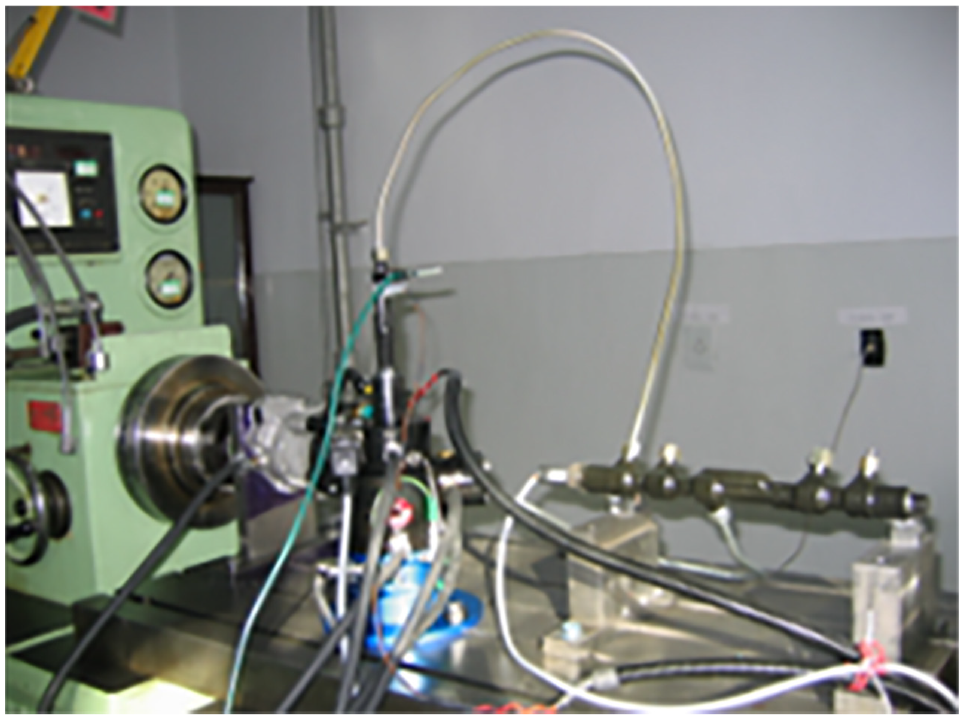
In this paper, the high-pressure common rail system of 10 cylinder diesel engine is taken as the research object. In order to simplify the calculation, a bench of high-pressure common rail fuel supply system of 5 cylinder monorail diesel engine is built for research. The relevant parameters are shown in Table 1. The operating conditions are as follows: the engine speed is 3800 rpm, the circulating fuel injection quantity is 220 mm³, and the fuel injection pulse width is 0.398 ms. The average rail pressure in one working cycle is 185 MPa, and the fluctuation is less than 5%. The injector is named a–E. according to the injection sequence. The test bench adopts Bosch rail pressure sensor with sampling frequency of 1000 Hz and dewe43 signal acquisition module as data collector. This paper uses MATLAB R2016b to build various mathematical models. The operating environment is win10, and the workstation is configured as Intel c621 series chipset; Intel Xeon gold 6145 processor, 40 cores, 80 threads, main frequency 2.0 GHz, maximum Rui frequency 3.7 GHz; 128 GB memory; NVIDIA gt1030, 2 GB graphics card. The fuel injector is shown in Figure 2 and the test bench is shown in Figure 3.

Table 1.

High pressure common rail system parameters.

Part	Parameter name	Numerical value
Rotor oil pump	Rotating speed (rpm)	600–2800
	Plunger diameter (mm)	8
	plunger stroke (mm)	12
	bearing clearance (mm)	0.04–0.07
	Plunger pair fitting clearance (mm)	0.002–0.004
	Inlet valve type	Poppet valve
	Outlet valve type	Ball valve
Common rail tube	total length (mm)	720
	Common rail tube inner diameter (mm)	14
	Inner diameter of high pressure oil pipe (mm)	3
fuel injector	Control valve lift (mm)	0.03
	Inlet hole diameter (mm)	0.28
	Outlet hole diameter (mm)	0.30
	Needle lift (mm)	0.2
	Number of nozzles	12
	Nozzle diameter (mm)	0.22
	Calibration cycle fuel injection quantity (mm³)	220
	Calibration injection duration (ms)	≤1.45
	Nozzle pressure chamber volume (mm³)	0.134

Figure 2.

Fuel injector.

Figure 3.

Common rail system test diagram.

According to the common faults and classification of oil supply system of high pressure common rail diesel engine, four operating states are selected, one of which is normal operation state, and three are fault state. The four states are: normal state, delayed injection state of injector C, oil leakage state at the inlet of common rail pipe and oil leakage state at the inlet of injector C, respectively. The above four states are named state 1–state 4 respectively. In this paper, the rail pressure data is pre processed with reference to the method proposed by Li et al. To improve the quality of rail pressure signal. The rail pressure signal is shown in Figure 4.⁸

Figure 4.

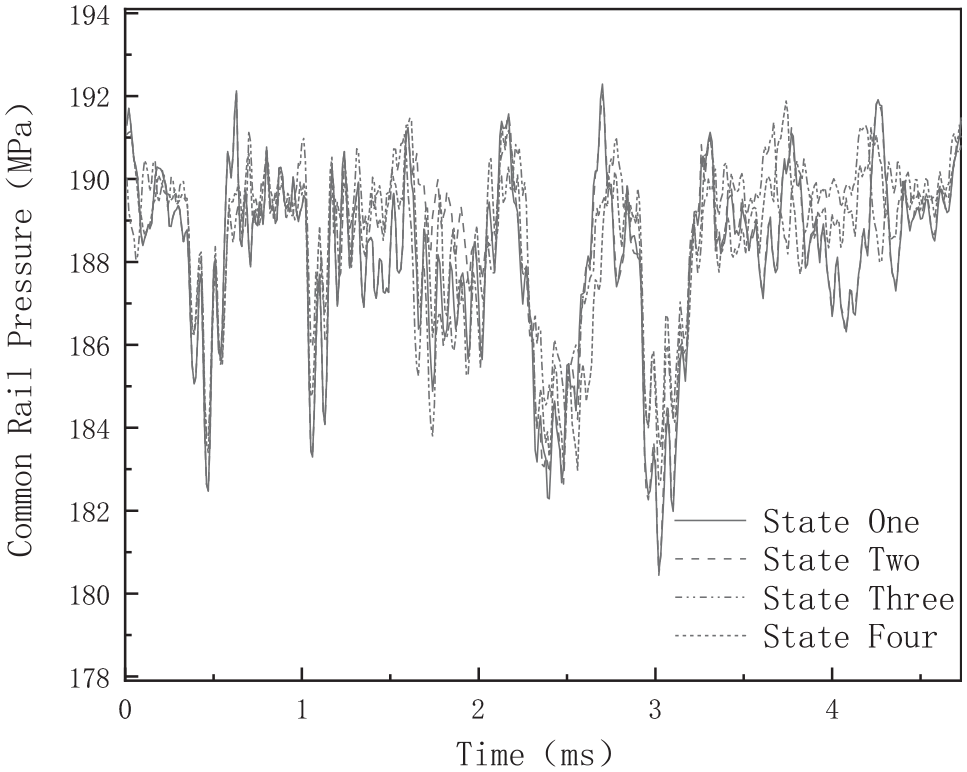
Rail pressure signals in different operating states.

In order to accurately extract the eigenvalues of rail pressure signal, the rail pressure signal is decomposed into different IMF by EEMD, and the extracted multiple energy eigenvalues are constructed as energy eigenvectors for fault diagnosis.

EEMD is a method based on EMD to decompose signals into intrinsic modal functions. By adding white noise signal to the original signal, the signals of different time scales are distributed to the appropriate reference scale. After several times of averaging to offset the noise, the final result is obtained by integrating the mean value. EEMD solves the mode aliasing problem of EMD by using the uniform distribution of white noise signal spectrum, further improves the decomposition accuracy, and accurately retains the characteristics in the original data.

The purpose of EEMD is to decompose a signal into n IMF and a residual. Among them, each IMF needs to meet the following conditions:

In the whole data range, the number of local extreme points and zero crossings must be equal, or the difference number must be at most 1.

At any time, the average value of the envelope of the local maximum (upper envelope) and the envelope of the local minimum (lower envelope) must be zero.

If a signal meets the following characteristics:

The signal has at least one maximum and one minimum.

The time scale characteristic of signal is determined by the time scale between two extreme points.

Then this signal can be EEMD.

Set M as the total number of expected EMD, m as the current number of EMD, and construct m different white noise signals for use. After all m times of decomposition are completed, the mean value of IMF corresponding to each stage obtained by m times of EMD is the final IMFs obtained by EEMD. The decomposition flow chart is shown in Figure 5.

Figure 5.

EEMD flow chart.

In the process of fitting the curve to get the upper and lower envelope, this paper uses cubic spline interpolation curve to construct the envelope.¹¹ Set interval $[a, b]$ . There are: $a = x_{0} < x_{1} < \dots < x_{n} = b$ , then for the interpolation function $s (x)$ . The following conditions shall be met:

For all internal nodes, the left and right limits of the interpolation function are equal and fixed.

For all internal nodes, the left and right limits of the first derivative are zero.

The interpolation function value of the head and tail nodes is fixed and the first derivative is zero.

According to the decomposition steps in this section, EEMD is performed on the rail pressure signals from state 1 to state 6 respectively, as shown in Figure 6(a)–(b) is the sixth order IMF component and spectrum decomposed from state 1 to state 6. It can be clearly seen that the frequency of each order IMF component is clear and the signal aliasing is not serious.

Figure 6.

Sixth-order IMF components and frequency spectrum of the state one rail pressure signal: (a) IMF and (b) spectrum.

In this paper, the IMF component with the largest zero crossing slope ratio of adjacent curves is selected as the separated IMF, which means that the signal contribution of this IMF component decreases suddenly. Compare the zero crossing rates of the sixth order IMF components from state 1 to state 6 respectively. As shown in Figure 7, the slope ratio of the number of zero crossings of imf1 to imf6 components of state 1 to imf1 to imf5 components is shown. It can be seen from the figure that the maximum slope ratio can be obtained at imf3. The slope ratio of the number of zero crossings of imf1–imf6 components and imf1–imf5 component signals in the other three states is similar to that in state 1, and the maximum slope ratio appears at imf3. Therefore, imf1, imf2, and imf3 components are used to extract eigenvalues.¹²

Figure 7.

The number of zero-crossing points and slope ratio of each IMF component.

The energy of each IMF component represents the energy of the signal within this frequency, so there is a mapping relationship between the signal and energy, which can be used as the basis of fault diagnosis. Here, the corresponding energy is extracted for imf1 and imf2 to construct the feature vector. Energy of each IMF component $E_{i}$ is:

E_{i} = \int_{0}^{T} c_{i}^{2} dt i = 1, 2, 3

(1)

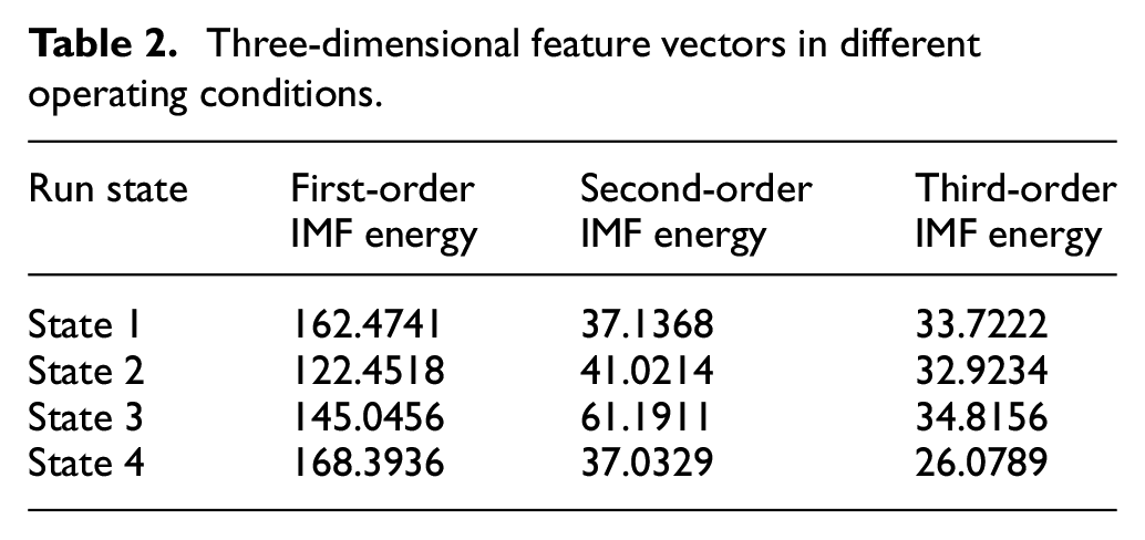
In equation (1) $E_{i}$ represents the energy of the ith IMF, $c_{i}$ represents the value of the ith IMF curve.

Table 2 shows the three-dimensional eigenvectors composed of the first three order IMF energy of rail pressure signals in four states after EEMD processing.

Table 2.

Three-dimensional feature vectors in different operating conditions.

Run state	First-order IMF energy	Second-order IMF energy	Third-order IMF energy
State 1	162.4741	37.1368	33.7222
State 2	122.4518	41.0214	32.9234
State 3	145.0456	61.1911	34.8156
State 4	168.3936	37.0329	26.0789

In order to verify the accuracy of the anti-interference model proposed in this paper, multiple groups of data need to be collected for classification training and testing. According to the above, 40 groups of rail pressure signals are collected as training samples for four operating states: normal state, delayed injection state of injector B, oil leakage state at the inlet of common rail pipe and oil leakage state at the inlet of injector B.

In order to construct the contour, it is necessary to reduce the discrete points of high latitude to two dimensions. In this paper, principal component analysis (PCA) is used to reduce the dimension of three-dimensional feature vector to two-dimensional eigenvalue vector, which is a common linear dimension reduction method. It maps high-dimensional data to low-dimensional space through some linear projection, and expects the maximum variance of data in the projected dimension. In this way, fewer data dimensions are used and more original data points are retained. PCA is a linear dimensionality reduction method with the least loss of original data information. After dimensionality reduction, the distribution is closest to the original data, and it can reduce the dimension of discrete points to any dimension.

The steps of dimensionality reduction using PCA can be expressed as follows:

Select a feature, average each feature, and subtract the average value from the original data to the new centralized data.

Find the characteristic covariance matrix.

According to the covariance matrix, the eigenvalues and eigenvectors are obtained.

The eigenvalues are arranged in descending order, the corresponding eigenvector is given, and the principal component is selected to calculate the projection matrix.

The reduced dimension data is obtained according to the projection matrix.

Extract the first three order IMF energy from the rail pressure signal of the training sample to form a three-dimensional feature vector. After dimensionality reduction, the box diagram is obtained, as shown in Figure 8, the abscissa in the figure represents state 1 to state 4 from left to right, and the two-dimensional diagram of energy distribution is drawn, as shown in Figure 9. It can be seen from the above figure that after EEMD decomposition, energy eigenvalue extraction and dimension reduction, the energy eigenvectors of the four states are clearly distinguished. The fault diagnosis model based on SVM is shown in Figure 10.

Figure 8.

Two dimensional eigenvector box diagram.

Figure 9.

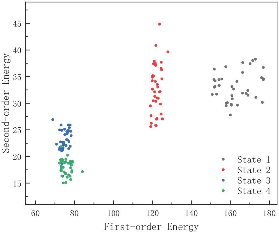
Schematic diagram of two-dimensional feature vector.

Figure 10.

Fault diagnosis model based on SVM.

This paper will build an anti-interference classification model based on 160 groups of training samples in four states and the fault diagnosis model.

Construction of anti-interference classification model

As can be seen from Figure 8, the distribution of eigenvalues of state 1 and state 2 is relatively independent for other states, while the eigenvalues of state 3 and state 4 cross together. It is expected that after complete fusion, three regions A, B, and C as shown in Figure 11 can be formed, in which a is composed of state 1, B is composed of state 2, and C is composed of state 3 and state 4. This section will show the whole process of constructing the anti-interference classification model: establishing the independent boundary of each state – boundary fusion to form the region – establishing the regional relaxation boundary – establishing the anti-interference classification model.

Figure 11.

Schematic diagram of expected fusion area of two-dimensional feature vector.

Construction of state boundary

In order to extract the boundary points of each state, this paper adopts the alpha shapes algorithm proposed by Edelsbrunner H. which is a simple and effective method to extract the boundary points quickly. It overcomes the disadvantage of the influence of the shape of the boundary points of the point cloud, and can extract the boundary points quickly and accurately. For two-dimensional discrete points of arbitrary shape, make a radius of $γ$ . The circle is rolled around it. If rolling circle radius $γ$ is small enough, each point in the discrete point is a boundary point; If properly increased $γ$ . To a certain extent, make it roll only on the boundary points, then the rolling track is the boundary of discrete points. The working diagram of the algorithm is shown in Figure 12.

Figure 12.

Schematic diagram of 2D discrete point boundary extraction.

The calculation steps of the algorithm are:

When the rolling radius is $γ$ . For including $z$ two dimensional discrete point set of point $P (p 1, p 2, \dots pz)$ . Any point in the $p (x, y)$ , find with $p$ distance in $2 α$ . All points within form a point set $Q (p_{1}, p_{2}, \dots, p_{n})$ .

Pick point $Q$ any point in the set $p_{i} (x_{i}, y_{i}), i \in (1, n)$ , calculate the corresponding center coordinates $R_{1} (x_{i}^{1}, y_{i}^{1})$ and $R_{2} (x_{i}^{2}, y_{i}^{2})$ :

\begin{matrix} x_{i}^{1} = x + \frac{x_{i} - x}{2} - H (y_{i} - y) \\ y_{i}^{1} = y + \frac{y_{i} - y}{2} - H (x_{i} - x) \\ x_{i}^{2} = x + \frac{x_{i} - x}{2} + H (y_{i} - y) \\ y_{i}^{2} = y + \frac{y_{i} - y}{2} + H (x_{i} - x) \end{matrix}

(2)

Where:

\begin{matrix} H = \sqrt[2]{\frac{α^{2}}{S^{2}} - \frac{1}{4}} \\ S^{2} = {(x_{i} - x)}^{2} + {(y_{i} - y)}^{2} \end{matrix}

(3)

3. If for a point set $Q$ division $p_{i}$ every point outside, its to $R_{1}$ or $R_{2}$ all distances are greater than $γ$ , indicates $p (x, y)$ is the boundary point.

4. If for a point set $Q$ division $p_{i}$ every point outside, its to $R_{1}$ or $R_{2}$ . The distance is not all greater than $γ$ , then traverse the point set $Q$ replace all points with $p = p_{c}, c \in (1, n)$ , return to step 2 for calculation. If present $p_{c}$ in the conditions of step 3 are met, this point $p_{c}$ . As boundary points, judge the point set $Q$ . The next point in the; If point set $Q$ , there are no points in the that comply with step 2. It indicates that there are no boundary points in this set. Repeat step 1 until traversal $P$ up to all points in the.

After the above steps, the two-dimensional discrete point set $P$ can be obtained . Boundary point set $T (t_{1}, t_{2}, \dots, t_{m}), m \leq z$ , Boundary circle point set $R (r_{1}, r_{2}, \dots, r_{m}), m \leq z$ .

Each state boundary constructed by the above method is shown in Figure 13.

Figure 13.

Schematic diagram of state boundary construction.

Boundary fusion and construction of relaxed boundary

As can be seen from Figure 13, the boundaries of state 1 and state 2 are relatively independent of other states, while the boundaries of state 3 and state 4 are intertwined. Therefore, the boundaries of state 3 and state 4 are fused here. In addition to the states where the boundaries intersect, the states where the boundaries do not intersect but are too close are also fused. For any state $α_{m}$ , if its boundary line and state $α_{n}$ . The intersection or minimum boundary distance is less than the fusion coefficient $μ$ , then the two states are fused and regarded as states $α_{mn}$ . And build according to the steps in Section 3.1 Repeat this step until no boundary lines of any state intersect or the small boundary distance is less than $μ$ . So far, the region boundary obtained by this step is shown in Figure 14.

Figure 14.

Schematic diagram of regional boundary construction.

At this time, if a point is not in the state $α_{x}$ , which cannot be said that this point must not belong to the state $α_{x}$ , this point may be a state $α_{x}$ . The singular value of or not included due to insufficient samples, so the boundary of each state should be extended.

For any state $α_{x}$ , it consists z points of two dimensional discrete point set composed of points $P (p_{1} (x_{1}, y_{1}), p_{2} (x_{2}, y_{2}), \dots p_{z} (x_{z}, y_{z}))$ form, $R$ is boundary circle points composed of $h$ points. The boundary circle point set composed of points is set in its boundary segment set $L$ inner point $Q (x, y)$ the minimize equation (4).

| \sum_{z}^{i = 1} [\begin{matrix} x_{i} - x \\ y_{i} - x \end{matrix}] |

(4)

This problem can be solved by genetic algorithm and other optimization algorithms. The solution and optimization process of this problem will not be repeated in this paper.

Select $δ_{x}$ as the status $α_{x}$ boundary relaxation variable, obtaining the status through the following steps $α_{x}$ relaxed boundary:

1. Set of line segments at boundary $L$ select a line from the list $l_{mn} = (p_{m} (x_{m}, y_{m}), p_{n} (x_{n}, y_{n}))$ calculate the relaxation distance $δ_{x} \sqrt[2]{{(x_{m} - x)}^{2} - {(y_{m} - y)}^{2}}$ and $d_{n} = δ_{x} \sqrt[2]{{(x_{n} - x)}^{2} - {(y_{n} - y)}^{2}}$ .

2. Through segment $l_{mn}$ corresponding boundary Center $r_{mn} (x_{mn}, y_{mn})$ , determine the relaxation vector $\vec{a_{mn}} = [\begin{matrix} x_{mn} - \frac{x_{m} + x_{n}}{2} \\ y_{mn} - \frac{y_{m} + y_{n}}{2} \end{matrix}]$ .

3. Calculated $p_{m}$ and $p_{n}$ by equation (5), corresponding relaxed boundary points $p_{m}^{mn} (x_{m}^{δ}, y_{m}^{δ})$ and $p_{n}^{mn} (x_{n}^{δ}, y_{n}^{δ})$

[\begin{matrix} \frac{x_{mn} - \frac{x_{m} + x_{n}}{2}}{| \vec{a_{mn}} |} \\ \frac{y_{mn} - \frac{y_{m} + y_{n}}{2}}{| \vec{a_{mn}} |} \end{matrix}] = [\begin{matrix} \frac{x_{m}^{mn} - x_{m}}{d_{m}} \\ \frac{y_{m}^{mn} - y_{m}}{d_{m}} \end{matrix}] = [\begin{matrix} \frac{x_{n}^{mn} - x_{n}}{d_{n}} \\ \frac{y_{n}^{mn} - y_{n}}{d_{n}} \end{matrix}]

(5)

4. Loop from step 1 to step 3 until you traverse the set Medium $L$ A boundary line $h$ . Can get $h$ line new relaxed boundary line for two adjacent segments $p_{a}^{ab} p_{b}^{ab}$ and $p_{b}^{bc} p_{c}^{bc}$ , if they intersect $p_{ac}^{δ}$ , replace the relaxed boundary line with $p_{a}^{ab} p_{ac}^{δ}$ and $p_{ac}^{δ} p_{c}^{bc}$ , if they do not intersect, a new relaxed boundary line is added $p_{b}^{ab} p_{b}^{bc}$ . From which the status is obtained $α_{x}$ relaxed boundary of $L^{δ}$ .

The two-dimensional feature vector set is constructed by the above method $α$ . The relaxation boundary of is shown in Figure 15.

Figure 15.

Schematic diagram of relaxation boundary.

Construction of classification model

In order to obtain the point set samples that do not belong to the known state, it is necessary to generate random points in a certain range. In order to make the generated points more evenly distributed, the fixed sized candidate set art (fscs-art) algorithm is used to generate random points. This is an adaptive random testing algorithm based on Art (adaptive random testing). Its core idea is to generate a candidate test set first. The shortest distance set is composed of the shortest distance between each individual in the candidate test set and each individual in the test set, and then the maximum distance in the shortest distance set is updated to the test set. It can be represented by equation (6).

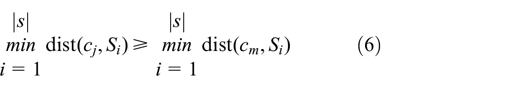
\begin{matrix} | s | \\ \min \\ i = 1 \end{matrix} dist (c_{j}, S_{i}) \geq \begin{matrix} | s | \\ \min \\ i = 1 \end{matrix} dist (c_{m}, S_{i})

(6)

The distance between a and b is representative by $dist (a, b)$ . As shown in Figure 16, taking $x \in (0, 100), y \in (0, 100)$ as an example, the comparison between the two-dimensional array obtained by art and the two-dimensional array obtained by random number generator. As can be seen from the figure, the data generated by art is more evenly distributed.

Figure 16.

Comparison of randomly generated two-dimensional arrays: (a) art and (b) randomly generated.

In order to make the point set evenly distributed in the non covered area, when initializing the candidate test set V, filter the points in the test set and eliminate the points in all covered areas. The steps are as follows:

For each candidate test set point, for a certain state, select a random direction to construct ray a, and construct ray b in the opposite direction at the same time.

When the rays on both sides do not pass through the endpoint of the state boundary. If there are odd intersections between ray a or ray b and the boundary of a state, the point is considered to be within this state, and the point is removed from the candidate test set. Return to step 1, reselect the state and build a new ray until the points of the candidate test set are determined.

When a side ray passes through the endpoint of the state boundary, return to step 1 and reconstruct the ray for this state.

The SVM dichotomy model using Gaussian kernel function is constructed for the obtained covered area point set and non covered area point set. This is a kernel function mainly used in the case of linear indivisibility. Its parameters are many and the classification results are very dependent on the parameters. Good results can be obtained when solving the classification problem with small feature dimension and normal sample number. The disadvantage is that finding the appropriate parameters often takes a lot of time and depends on manual selection. Thus, the trained anti-interference model can be obtained.

Cluster analysis

After classification by anti-interference model, for a certain area $α$ , three closed curves appear in the training space: boundary line, hyperspace plane and relaxed boundary. The space formed by it can be divided into space, space, space and space, and its relationship is shown in Figure 17, in which $a \in A, b \in B, c \in C$ .

Figure 17.

Schematic diagram of relationship between area and boundary.

For any data, there are only three situations: p

$p \in A$ At this time, it is considered that the data probability belongs to the status $α$ , classify the data for fault diagnosis.

$p \in B$ At this time, it is considered that the data has a high probability and belongs to state $α$ , no fault diagnosis classification is performed on the data, but it is marked as status $α$ . Singular value of.

$p \in D$ or $p \in C$ . At this time, it is considered that the data probability does not belong to the status $α$ , do not classify the data for fault diagnosis.

Through the corresponding steps in Section 3.3, any feature vector can be classified in the above three cases. For 1 and 3 cases, the specific status of the data will be accurately classified. For the second case, it is only marked as possible $α$ , but due to status $α$ . It may be formed by the fusion of multiple states, and this conclusion alone is not enough to make a clear analysis of the data. This paper introduces the concept of clustering in order to make a reference for the specific state analysis of data. This is a classification model that classifies some indicators according to certain standards (similarity, affinity, etc.), and it is a method to classify things with fuzziness.

In order to further accurate the possible state of data, this paper uses k-means algorithm to process data and state p and a. This is a hard clustering algorithm, which can strictly classify the identified objects into a specific category, and can better solve the data p either or problem faced in this paper. The calculation steps are as follows:

Set the number k of cluster centers and initialize the location of cluster centers $C^{0} = {c_{1}, c_{2}, \dots c_{k}}$ , input dataset X

Calculation $dis (c_{i}, x)$ , each data point can get k distances. Select the nearest distance and classify the point into this class.

After classifying all points in the data set, calculate the center point of all points in each class as the new clustering center of this class $C^{new}$ .

If the iteration conditions are met, the clustering results are obtained. If not, repeat the second step.

In this paper, the iteration stop condition shown in equation (7) is used.

J (C) = \sum_{i = 1}^{K} \sum_{x \in c_{i}} dis {(c_{i}, x)}^{2}

(7)

Experiment and result analysis

At present, multiple groups of signals are collected for four operating states: normal state, delayed injection state of injector C, oil leakage state at the inlet of common rail pipe and oil leakage state at the inlet of injector C to form a verification set; In order to verify the anti-interference ability of the anti-interference classification model constructed in this paper, Add several signals of the fifth state and several meaningless signals (named state 6) to the verification set; in order to verify the classification ability of the anti-interference classification model constructed in this paper, select several singular values of four states to the verification set. State 5 is the wear state of the oil pump plunger, and its rail pressure signal is shown in Figure 18.

Figure 18.

Rail pressure signal in state V.

Thus, 20 state one signals (including two singular values), 20 state two signals (including one singular value), 20 state three signals (including two singular values), and 20 state four signals are obtained (including a singular value), 10 state five signals and 10 randomly generated meaningless signals constitute a verification set. The signals are numbered as 1–100 in sequence, in which the singular values are numbered as 19, 20 (state I), 40 (state II), 59, 60 (state III) and 80, respectively (state 4) the two-dimensional feature vector is constructed by the method in the second section above, and its eigenvalues are shown in Figure 19.

Figure 19.

Schematic diagram of characteristic values.

Input the above training set into the fault diagnosis model without anti-interference classification model to classify the operation state. The classification results are shown in Figure 20. The abscissa in the figure is the signal number of the training set, and the ordinates 1–6 represent state 1–state 6 respectively.

Figure 20.

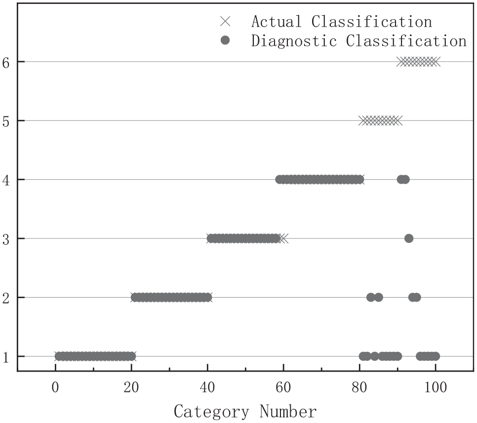
Classification results.

As can be seen from the above figure, the fault diagnosis model classifies all States into trained States, which leads to the classification of state 5 and state 6 to state 1 to state 4, respectively according to the set hyperspace plane. In state 5, two signals are classified in state 2 and eight signals are classified in state 1. In the face of the trained state, due to the existence of singular values, the signals of two state three are classified into state four.

As a comparison, input the above training set into the fault diagnosis model including the anti-interference classification model to classify the operation state, as shown in Figure 21, the abscissa in the figure is the signal number of the training set, and the ordinate is the screening result, where 1, 2, and 3 represent trained, singular value and untrained respectively. As shown in Figure 22, the diagnosis results combined with cluster analysis are shown, and the abscissa in the figure is the signal number of the training set; Ordinates 1–5 represent state I, state II, state III, State IV, and untrained state respectively; Red represents the singular value signal judging that it is in the trained state, which should be added to the training set for updating.

Figure 21.

Screening results.

Figure 22.

Classification and clustering results.

It can be seen from the figure that the fault diagnosis model with anti-interference classification model judges five of the six singular values correctly; 18 of the 20 interference states (state 5 and state 6) are judged correctly. Table 3 shows the accuracy analysis of the two fault diagnosis models.

Table 3.

Accuracy analysis.

Does not Include Anti-jamming Classification Model			Includes Anti-jamming Classification Model
Operational status diagnostics			Operational status diagnostics
State	Number of correct diagnoses/number of samples	Diagnosis accuracy rate/%	State	Number of correct diagnoses/number of samples	Diagnosis accuracy rate/%
1	20/20	100	1	20/20	100
2	20/20	100	2	20/20	100
3	18/20	90	3	19/20	95
4	20/20	100	4	20/20	100
5	0/10	0	5	10/10	100
6	0/10	0	6	8/10	80
Singular value			Singular value
State	Number of correct diagnoses/number of samples	Diagnosis accuracy rate/%	State	Number of correct diagnoses/number of samples	Diagnosis accuracy rate/%
1	0/2	0	1	2/2	100
2	0/1	0	2	1/1	100
3	0/2	0	3	1/2	50
4	0/1	0	4	1/1	100

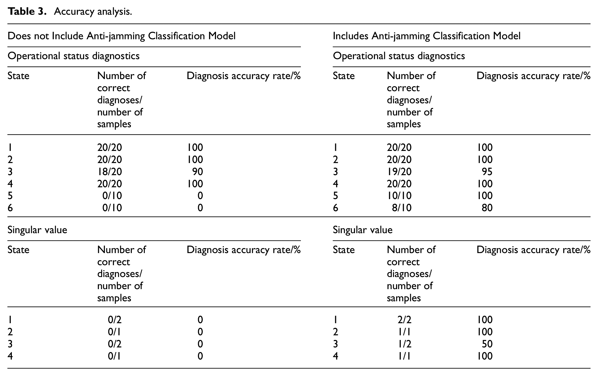
It can be seen from the Table 3 that the fault diagnosis model with anti-interference classification model has strong anti-interference ability and strong troubleshooting ability for untrained States, and its classification accuracy can reach 90%. It has strong classification ability for the singular values in the trained state, and at least 50% of the singular values can be selected to update the training set. At the same time, screening the samples in advance also helps to improve the diagnostic accuracy of the trained state, and the diagnostic accuracy is increased from 97.5% to 98.75%. From the experimental results, the addition of anti-interference classification model helps to improve the accuracy of fault diagnosis model of common rail system, and brings strong anti-interference and training set updating ability to the fault diagnosis model.

Conclusion

In order to improve the anti-interference ability and training set updating ability of the fault diagnosis model of high-voltage common rail system, the rail pressure signals under different operating states of high-voltage common rail system are obtained through bench test. The fault diagnosis model of high-voltage common rail system based on SVM is established through EEMD decomposition, energy eigenvector construction and dimension reduction processing. Based on alpha shapes algorithm and K-means algorithm, an anti-interference classification model composed of anti-jamming device and classifier is established. Compared with the fault diagnosis model without anti-interference classification model, the following conclusions can be obtained.

Compared with the fault diagnosis model without anti-interference classification model, the fault diagnosis model with anti-interference classification model has an ability to classify the untrained state. In the face of four trained states: normal state, delayed injection state of injector C, oil leakage state at the inlet of common rail pipe and oil leakage state at the inlet of injector C, and two untrained states: worn state and meaningless state of oil pump plunger, the fault diagnosis model with anti-interference classification model can classify the untrained state with a correct rate of 90%, most untrained states can be excluded.

Compared with the fault diagnosis model without anti-interference classification model, the fault diagnosis model with anti-interference classification model has an ability to update the training set. In the face of six singular values of four trained States, the fault diagnosis model with anti-interference classification model classifies five of them, and correctly classifies their possible subordinate states. The accuracy rate is 83.3%. It can be added to the training set of fault diagnosis model to update the training set.

Compared with the non-interference fault diagnosis model, the fault diagnosis accuracy of the fault diagnosis model with anti-interference classification model is slightly improved, which is due to the classification of singular values of trained states and cluster analysis.

To sum up, the anti-interference classification model for fault diagnosis of high-voltage common rail system proposed in this paper can effectively improve the anti-interference ability and training set updating ability of the fault diagnosis model, and can slightly improve the diagnosis accuracy of the fault diagnosis model for the trained state. Because it does not need to change the structure of the original fault diagnosis model, it can be added in front of any fault diagnosis model relying on eigenvector to improve its anti-interference ability and training set updating ability.

Footnotes

Handling Editor: Chenhui Liang

Declaration of conflicting interests

The author(s) declared no potential conflicts of interest with respect to the research, authorship, and/or publication of this article.

Funding

The author(s) received no financial support for the research, authorship, and/or publication of this article.

ORCID iD

Yaoyao Shi

References

Zhao

Research on high pressure common rail fuel injection quantity diagnosis based on rail pressure characteristics. PhD Thesis, Beijing University of Technology, China, 2020.

Qifeng

Research on key technology of fault diagnosis of high pressure common rail diesel engine. PhD Thesis, Kunming University of Science and Technology, China, 2020.

Zhao

Zhou

Yong

, et al. Experimental research on dynamic response of high-speed solenoid valve of common rail injector. J Harbin Eng Univ 2018; 39: 74–79.

Napolitano

Guido

Beatrice

, et al. Analysis of nozzle coking impact on emissions and performance of a Euro5 automotive diesel engine. SAE Int J Engines 2013; 6: 1801–1813.

Ikemoto

Omae

Nakai

, et al. Injection nozzle coking mechanism in common-rail diesel engine. SAE Int J Fuel Lubricants 2011; 5: 78–87.

Smith

Williams

Linking the physical manifestation and performance effects of injector nozzle deposits in modern diesel engines. SAE Int J Fuel Lubricants 2015; 8: 344–357.

d’Ambrosio

Ferrari

Diesel injector coking: optical-chemical analysis of deposits and influence on injected flow-rate, fuel spray and engine performance. J Eng Gas Turbine Power 2012; 134: 062801.

Tiexiong

, et al. Research on a small sample fault diagnosis method for a high-pressure common rail system. Adv Mech Eng 2021; 13: 15–27.

Awrangjeb

Using point cloud data to identify, trace, and regularize the outlines of buildings. Int J Remote Sens 2016; 37: 551–579.

10.

Xiaojun

Fang

Extraction of contour feature line of scattered point cloud based on morphology. J Tongji Univ (Nat Sci Ed) 2014; 42: 1738–1743.

11.

Wenjing

Shaoning

Qiu

, et al. Multi-density discrete point group boundary detection by convex hull shrinkage method. Surv Map Sci 2014; 39: 126–129.

12.

Yunfan

Debao

Guang

, et al. Research on building contour extraction from point cloud by double threshold alpha shapes algorithm. J Changjiang Acad Sci 2016; 33: 1–4.

13.

Wang

, et al. Automatic extraction of building boundaries using aerial LiDAR data. J Appl Remote Sens 2016; 10: 016022.

14.

Zhan

Zhang

Research on the integrated algorithm of point cloud boundary extraction and triangular mesh generation. Comput Simul 2013; 30: 272–275.

15.

Yang

Liyan

Chunxia

, et al. Variable radius alpha shapes extraction of building contours from airborne LiDAR point cloud. Chinese J Image Graph 2021; 26: 910–923.

16.

Zhou

Yingnan

Yongchao

Overview of data processing and analysis algorithms for big data. J Nanjing Univ Aeronaut Astronaut 2021; 53: 664–676.

17.

Wang

Hilbert-Huang transform and its application in non-stationary signal analysis. PhD Thesis, North China Electric Power University (Beijing), China, 2008.

18.

Xuejiao

Research on vibration fault diagnosis of rotating machinery based on support vector machine. Electron Des Eng 2016; 24: 104–107.

19.

Shalev-Shwartz

Singer

Srebro

, et al. Pegasos: primal estimated sub-gradient solver for SVM. Math Program 2011; 127: 3–30.

20.

Zhuang

WANG

Crammer

Vucetic

Breaking the curse of kernelization: budgeted stochastic gradient descent for large-scale SVM training. J Mach Learn Res 2012; 13: 3103–3131.

21.

Nguyen

, et al. Approximation vector machines for large-scale online learning. J Mach Learn Res 2017; 18: 3962–4016.

22.

Tang

Jiabin

, et al. Improved bridge crack extraction combined with mask uniform light and K-means clustering. Electron Meas Technol 2021; 13: 1–17.

23.

Fahim

Salem

Torkey

, et al. An efficient enhanced k-means clustering algorithm. J Zhejiang Univ Sci A 2006; 7: 1626–1633.

24.

Lai

JZC

Huang

Liaw

YC.

A fast k -means clustering algorithm using cluster center displacement. Pattern Recognit 2009; 42: 2551–2556.

25.

Zhao

Liang

Dang

A stratified sampling based clustering algorithm for large-scale data. Knowl Based Syst 2019; 163: 416–428.

26.

Hadian

Shahrivari

High performance parallel K-means clustering for disk-resident datasets on multi-core CPUs. J Supercomput 2014; 69: 845–863.

27.

Mautz

Plant

, et al. Discovering non-redundant K-means clusterings in optimal subspaces. In: Proceedings of the 24th ACM SIGKDD International conference on knowledge discovery & data mining, Berlin, Germany, 2018, pp.1973–1982. Dallas, TX: ACM.

28.

Dongdong

CHEN

Jiancheng

Zhang

. Unsupervised multi-manifold clustering by learning deep representation. In: Proceedings of workshops at the thirty-first AAAI conference on artificial Intelligence, San Francisco, CA, 2017, pp.385–391. San Francisco, CA: AAAI.

29.

Kobren

Monath

Krishnamurthy

, et al. A hierarchical algorithm for extreme clustering. In: Proceedings of the 23rd ACM SIGKDD International conference on knowledge discovery and data mining, Toronto, ON, 2017, pp.255–264. Dallas, TX: ACM.

30.

Monath

Dubey

Guruganesh

, et al. Scalable hierarchical agglomerative clustering. In: Proceedings of the 27th ACM SIGKDD Conference on knowledge discovery & data mining, Singapore, 2021, pp.1245–1255. Dallas, Texas: ACM.

31.

Erdem

Gündem

Tİ.

M-FDBSCAN: a multicore density-based uncertain data clustering algorithm. Turk J Electr Eng Comput Sci 2014; 22: 143–154.

Research on anti-interference and training set updating ability of fault diagnosis model of high voltage common rail system

Abstract

Keywords

Introduction

Decomposition of rail pressure signal, construction of eigenvector, and establishment of fault diagnosis model

Construction of anti-interference classification model

Construction of state boundary

Boundary fusion and construction of relaxed boundary

Construction of classification model

Cluster analysis

Experiment and result analysis

Conclusion

Footnotes

Declaration of conflicting interests

Funding

ORCID iD

References