Sage Journals: Discover world-class research

Abstract

In this paper, long short-term memory (LSTM) and Transformer neural network models were developed for classification of different conveyor belt conditions (loaded and unloaded). Comparative shallow models such as logistic regression, support vector machine and random forest were also developed and summarized. Six different-length belt pressure signals were analyzed: 0.2, 0.4, 0.8, 1.6, 3.2, and 5.0 s. Both LSTM and Transformer models achieved 100% accuracy using pressure raw signal. Furthermore, LSTM model reached the highest classification level with the shortest signals. Accuracy and F1-score of 98% and 100% were reached using only 0.8 and 1.6 s-length signals, respectively. Also, LSTM model performed training and testing procedures faster than Transformer. Random forest model demonstrated the best classification level using aggregated signal data with accuracy of 85% and F1-score for loaded and unloaded conditions of 85% and 69%, respectively. Loaded conveyor belt condition was significantly easier to classify than the unloaded one in all models. Only LSTM showed better classification recall for unloaded conveyor belt condition using short signal. Experimental research dataset CORBEL (Conveyor belt pressure signal dataset) and models are open-sourced and accessible on GitHub https://github.com/TadasZvirblis/CORBEL.

Keywords

Conveyor rubber belt classification machine learning logistic regression support vector machine random forest long short-term memory neural networks transformer neural networks

Introduction

This study is dedicated to the belt conveyors (CB), one of the many types of devices applied in industrial transportation systems. Conveyors are used in production process to ensure its efficiency in terms of timely transportation of loose materials or components and assembled units.¹ In industrial applications, new CB solutions may substantially reduce overall production costs.² However, due to lack of systems for real-time monitoring of CBs, interruptions in the manufacturing process may occur and generate additional expenses and losses.³

Research data obtained by some authors from metro-tomographic analysis showed that the initial damage of the inner structure of the CB occurred at the tensile load 2157 N.⁴ Under dynamic conditions, especially when sharp elements fall on the belt, much smaller tensions may cause damages and breakdowns. Therefore it was found important to perform experimental research on the belt tension under working conditions.

Within the Industry 4.0 framework, cyber-physical systems (CPS) gain increasing significance and are oriented to future realization of a CPS-based smart factories.⁵ The most recent CBs maintenance trends include creating monitoring systems which would be able to perform real-time data analysis with machine learning algorithms and further decision making.⁶ Such a CB-monitoring system can be integrated with a CPS due to introduction of Internet of Things (IoT).⁷ Moreover, in recent studies failure analysis of the belts employs virtual reality in order to achieve higher degree of sustainability.^8,9

The above-mentioned tasks can be performed by monitoring some critical elements of the conveyor. In some literature sources, electrical motor, gearbox, rollers, joints, and the belt itself are mentioned among the components that can be monitored and included to a diagnostic system.¹⁰ CB fault classification analysis includes a wide range of statistical and machine learning methods.

Simple statistical classification models were presented in several research works by Andrejova et al.^9,11,12 The same independent factors such as CB type, impactor type, and the drop height were used in all these studies. In the first article,¹¹ the authors presented classification analysis of four-conditions CB damage using naïve Bayes classifier which showed 78.8% classification accuracy. Later, the authors expanded their investigation by using additional models.¹² Decision tree and linear regression models showed identical accuracy of 81.5%. In the later research paper,⁹ Andrejova et al. presented four classification models: logistic regression, linear regression, decision tree, and naïve Bayes classifier. All the models showed identical accuracy of 85.0%. It should be noted that in their latest research paper the authors developed binary classification models.

For real-time monitoring of CBs, the measurement of audio noise was proposed,¹³ also by using acoustic camera that allows verification of correct operation of individual elements of CB by searching for improper frequencies in the analyzed spectrum during the operation.¹⁴ Other proposed solutions were multispectral visual inspection based on visible, mid-infrared, and far infrared images,¹⁵ and gearbox temperature measurement with training process in the statistics domain for complex decision making.¹⁶ An interesting solution was proposed involving application of magnetized steel cord when the changes of magnetic field are generated around the defects and the measurements of these changes provide information on the growing defects.¹⁷ However, existing methods either involve advanced devices and thus are very expensive, or provide signals of low reliability. For instance, application of permanent magnets embedded in CB identified by a semiconductor magnetic field sensor to inspect the belt¹⁸ generate additional costs of the belt preparation and its utilization after damage. On the other hand, impact of sharp material may lead to local anomalies that are not recognizable as a breakdown because perforation for all CB layers does not take place so that the belt cannot be unequivocally determined as suitable or unsuitable for operating condition.¹⁹

Some authors proposed CB monitoring system based on the combination of sound and thermal infrared image which is able to perform fault analysis of CB idlers.²⁰ This study developed gradient boost decision tree for classification of CB idler rolls’ faults which used Mel-frequency cepstral coefficients of acoustic signal. The proposed method achieved accuracy of 94.5% on the average.

Che et al.²¹ proposed a new method, named audio-visual fusion (AVF), for detecting longitudinal tear of CB. Authors used both visible light and microphone array to monitor CB in different running states. Mel-frequency cepstral coefficients, spectral centroid, short-time energy, zero crossing rate, and spectral roll-off were used for extraction of the audio feature and histogram of oriented gradient was used for extraction of the visual feature. Using K-nearest neighbors, support vector machine, and random forest algorithms the authors reached excellent accuracy of 93%–97%. However, the authors did not specify selection of their training and testing sets, therefore it is not clear if that accuracy level was reached by using unseen data.

Santos et al.²² presented binary classification models which use using CB images. This classification was performed using convolutional neural networks such as visual geometry group (VGG) network, residual network (ResNet) and densely connected convolutional network (DenseNet). The best average accuracy (89.8%) result was reached by using DenseNet model.

A comprehensive machine learning (ML) algorithms’ research was performed by Zhang et al.²³ The authors compared a wide range of sophisticated ML algorithms such as Faster R-CNN, SSD, RFBnet, M2det, Yolov3, and Yolov4. The Yolov3 algorithm was improved by the authors and reached a 97.3% precision on the average for four classes.

To summarize, despite many proposals of real-time devices for the monitoring of CB condition, no satisfactory measurement system has been built yet. In this research, we propose a novel solution of cheap and simple measurement method that is able to perform real-time monitoring tasks (see Figure 1). The objectives of this study are the following: (1) to develop ML models for distinguishing loaded and unloaded conditions of CB; (2) to identify optimal signal length of tensile pressure which enables achieving the best classification accuracy; (3) to evaluate the robustness of the best model for distinguishing CB conditions when CB and measurement system are not calibrated.

Figure 1.

Graphical abstract: Conveyor belt pressure signals are collected from CB work. The machine learning algorithms classify the load impact.

After the novel monitoring system had been projected, it was necessary to find the algorithm to identify reliably the collected signals for further decision making. The main contributions of this paper are:

For the first time, conveyor belt load status was classified using only belt tension signals;

Developed LSTM and transformer neural networks was able to classify conveyor belt load status with accuracy of 100%;

The sensitivity analysis was suggested to investigate the robustness of developed models;

The largest known conveyor belt pressure signal dataset was created and open-sourced.

The rest of the paper is organized as follows: first, CB real-time monitoring concept and mathematical methods are described; secondly, design and setup of our experiment are presented; later on, the results of the investigated algorithms of classification of CB pressure signal are presented, and conclusions close the article.

Methodology and data description

We started our study by creating CB-monitoring system based on strain gages. We have built an experimental rig (Figure 2) in order to simulate the work of CB. It consisted of two rollers with controllable rotational speed and a rubber belt between them. We used the belt of type EDV08PB-AS 2.0, 2 mm thickness, and adapted to work with rollers of minimal diameter of 30 mm. It had two inner layers and the PVC outer coating on the one side, which ensured the inner working force $F 1 % = 8$ N/mm.

Figure 2.

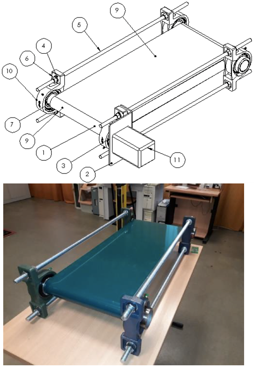
Schematic and the photo of the conveyor belt tension experimental rig: 1 – measurement system imbedded to the roller, 2 – reducer fixing plate, 3 – seal of the driving roller, 4 – tension regulation, 5 – leading thread, 6 – regulating nut, 7 – precise hollow shaft, 8 – rubber belt, 9 – strain gage on the roller surface, 10 – bearing, 11 – motor reducer.

The experimental rig enabled initial adjustment of the tension in order to achieve similar pressing forces on the roller at both sides of the belt width. In the middle of the belt width, the pressing force is always slightly higher. In this way, the system with strain gages solved several problems indicated by other researchers who investigated belt tension²⁴ and the belt mistracking during conveyor’s operation.²⁵

Our test campaign included measuring static tension under 2 kg load in different points of the CB and measurements in dynamic conditions. The latter conditions presumed the range of the linear belt speeds between $ν_{1} = 0.5$ and $ν_{\max} = 1.7$ m/s, which corresponded with the typical conditions of industrial transportation of the small components. The tension of the moving belt was measured both under loaded and unloaded conditions.

CB-monitoring system concept and calibration issue

The main idea of our novel concept was to place strain gages directly on roller’s surface making them the object of the tension-dependent pressuring force from the belt. The unit consisted of two strain gages, one in the middle of the roller’s length and the other at its end, signal-receiving and transmitting system, and the dedicated software for data processing and presentation. After the initial tests, strain gages CP 152 NS were found to be optimal.²⁶ Their nominal sensitivity was 0.5–0.8 mV/V, sampling frequency up to 20,000 Hz, and response time was 5 µs, what qualified the gages to perform dynamical measurements.

The strain gages, subject to the pressing force from the CB, were connected with electronic system placed in the hollow roller. The as-formed measurement system was able to measure the belt pressing force F continuously, as well as to collect and transmit data through a Bluetooth port. The data received by the computer were then processed in the real-time mode using a specialized program based on the LabView software.²⁷

However, before the strain gages could be applied properly, it was necessary to perform relevant calibration procedure. We decided to use a well-equipped laboratory of Radwag Company in Radom, Poland in order to minimize the impact of reference weights’ uncertainty, reading resolution, approximation error, and environmental conditions on the calibration uncertainty. It was also necessary to build special instrumentation providing repeatable contact conditions between the standard weight and the surface of the calibrated strain gage, as well as stable vertical movement able to transmit the force directly on the gage surface. After calibration in fully repeatable conditions with weights from 0.5 up to 10 kg, the strain gage characteristics were approximated as a polynomial with maximum error of conductance 7.73 [μS] determined with expanded uncertainty $U_{0.99} = 0.75$ [μS], assuming 99% level of confidence and corresponding coverage factor $k = 3$ .²⁸

Data acquisition

The strain gages with working area diameter of 16 mm were placed on the one side of the roller, so that they would be subject to the pressing force only when this particular side was under the belt. Thus, the gages emitted the signals of pressuring force only during half of the roller’s revolution time. Theoretically, assuming steady distribution of inner tensions in the belt, the signals would follow certain predictable pattern shown in Figure 3, where each rotation corresponds with a cyclic signal indicating a relevant pulse of pressure on the strain gage. However, in reality, very complex dynamical distribution of inner tensions resulted in certain differences between the shape of the pulses and in the forms of the pulses itself, as it is shown in Figure 3. Additional attention was paid to the maxima distinguishable at the beginning of a pulse and in its middle area.

Figure 3.

Conveyor belt tension signals of both strain gages.

The curves in Figure 4 were clipped peak-by-peak and centered by their starting point. It can be seen in Figure 4 that, on the average, load signals had higher tension peak values (see bold red vs blue curves). However, any time moment of the at curve shows that no-load/load distributions overlapped to such an extent that even their means were slightly shifted, and the curves were inseparable since both distributions totally overlapped. It is worthy to note that under no-load the curves were distributed with higher variation than under load condition. This also lead to conclusion that the curves, except for their shape, were inseparable at any time moment.

Figure 4.

Conveyor belt tension peak.

We chose a 400 Hz unified sampling frequency for the experiments. It corresponded with 140 samples per revolution at the minimum rotational speed of 159 rpm (for linear belt speed $ν_{1} = 0.5$ m/s) and 45 samples per revolution at the maximum rotational speed of 540 rpm (linear belt speed $ν_{max} = 1.7$ m/s). The experiment design was created based on the time stamps as follows: for the first 5 s there was no load, then for 15 s — load of 2 kg and for the last 5 s — no load (see Figure 3). Such experimental design allowed easy and quick data labeling based on fixed time stamps when preparing data for ML models. A special program based on the LabView software updates the plot each time when new data appear in the serial port buffer after initializing the measurement. There is a possibility to remove new data manually or stop recording them at any time. Operator can choose to export data to Excel file for additional analysis or to archive it. In the industrial monitoring system, all the data are planned to be archived and available for authorized users. Elsewhere in this publication, we define the dataset of collected data as CORBEL (Conveyor belt pressure signal dataset).

Machine learning methods

In this section, we cover the supervised ML methods and methodology used in our experiments. In this subsection $Y$ will be treated as CB load status and independent variable $X$ should be treated as input variable, that is, CB tension signal. Realizations (load target class/dependent variable) of $Y$ and $X$ are defined as $y$ and $x$ , respectively.

Logistic regression

Logistic regression model is commonly used for solution of binary classification problems. For binary response models, dependent variable $Y$ can take one of two possible values of the experiment outcome $Y \in {0, 1}$ . Suppose $X \subset R^{d}$ is a vector of explanatory (independent) variables, $x$ is a vector of observed vector $X$ and $P (Y = 1 | X = x)$ is the response probability to be modeled. Then logistic regression model takes the form ²⁹:

\begin{matrix} π (x) = P (Y = 1 | X = x) \\ = \frac{\exp (α + β_{1} x_{1} \dots + β_{d} x_{d})}{1 + \exp (α + β_{1} x_{1} + \dots + β_{d} x_{d})}, \end{matrix}

(1)

where $α$ is the intercept parameter and $β = (β_{1}, \dots, β_{d})^{T}$ is the vector of slope parameters.

Support vector machine

Support vector machine (SVM) model is widely applied for classification tasks in many research fields: text categorization, image classification, bioinformatics, fault detection, and other.³⁰

Assume that a dataset consists of pairs:

({\vec{x}}_{1}, y_{1}), ({\vec{x}}_{2}, y_{2}), \dots, ({\vec{x}}_{n}, y_{n}),

(2)

where ${\vec{x}}_{i} \in R^{d}$ and $y_{i} \in (+ 1, - 1)$ , $i = 1, 2, \dots, n$ . There is an infinite number of hyperplanes ${\vec{w}}^{T} x_{i} + b = 0$ that can separate data into two classes and there is only one hyperplane that separates data with a maximum margin. The latter hyperplane is called optimal separation hyperplane.

In order to estimate the parameters, Lagrangian formulation is used:

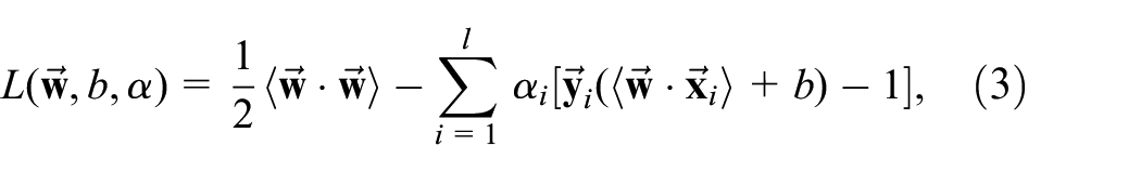
L (\vec{w}, b, α) = \frac{1}{2} 〈 \vec{w} \cdot \vec{w} 〉 - \sum_{i = 1}^{l} α_{i} [{\vec{y}}_{i} (〈 \vec{w} \cdot {\vec{x}}_{i} 〉 + b) - 1],

(3)

where $α_{i}$ are the Lagrange’s multipliers, and 〈·〉 - is dot product.

Random forest

Random forest is a classification model which enables a typical ensemble learning algorithm with a large number of decision trees.³¹ First, selected number $k$ of weak classifiers of decision tree $g_{j} (x^{*, j} | ϕ_{j}), j = 1, \dots, k$ with given depth $w$ and number of variables $l$ is constructed on random subset of variables $x^{*, j} \subset R^{l} \subset R^{d}$ . Afterward, the ensemble of weak classifiers is considered to construct the final model.

Long short-term memory

In deep learning, the problems of sequential and time series data $X = (x_{1}, x_{2}, \dots, x_{T})$ are very often approximated by recurrent neural networks.³² LSTM³³ is one of the prevailing models in the field of time series which relies on the combination of gate mechanism and state updates. The states of LSTM make a pair of hidden state vectors $(c_{t}, h_{t})$ .

After receiving new data input $x_{t}, t = 0, \dots, T$ , LSTM updates hidden state vector $h_{t - 1}$ to a new cell state ${\tilde{c}}_{t}$ and gate transformations are applied to calculate new variables $i_{t}$ , $f_{t}$ , and $o_{t}$ , which are known as input, forget, and output gates, respectively. The input gate $i_{t}$ has an interpretation of integration of cell vector ${\tilde{c}}_{t}$ into $c_{t}$ . The forget gate $f_{t}$ has an interpretation of integration of $c_{t - 1}$ and the output gate $o_{t}$ transforms cell $c_{t}$ into a new hidden state $h_{t}$ :

i_{t} = σ (ψ_{1, i} x_{t} + ψ_{2, i} h_{t - 1} + b_{i}),

(4)

f_{t} = σ (ψ_{1, f} x_{t} + ψ_{2, f} h_{t - 1} + b_{f}),

(5)

o_{t} = σ (ψ_{1, o} x_{t} + ψ_{2, o} h_{t - 1} + b_{o}),

(6)

{\tilde{c}}_{t} = \tanh (ψ_{1, c} x_{t} + ψ_{2, c} h_{t - 1} + b_{c}),

(7)

c_{t} = f_{t} ⊙ c_{t - 1} + i_{t} ⊙ {\tilde{c}}_{t},

(8)

h_{t} = o_{t} ⊙ \tanh (c_{t}),

(9)

where ⊙ denotes element-wise multiplication, $σ$ denotes sigmoid, $\tanh$ denotes hyperbolic tangent activations and $ψ$ denotes the unknown weights estimated from data. A fully connected layer $y = softmax (ψ h_{t} + b)$ is selected is an output for the many-to-one classification model.

Transformer neural network

Transformer neural networks³⁴ become state-of-the-art technique in natural language processing,³⁵ speech recognition,³⁶ time series³⁷, and many more sequential tasks.

Transformer’s mathematical model consists from multiple transformations: attention blocks, multi-head attention blocks, and fully connected layers.³⁴ The attention transformation $Attention (X) : R^{d_{x}} \to R^{d_{v}}$ is used to transform the sequence $x = (x_{1}, x_{2}, \dots, x_{d_{x}})$ to lower dimension. First, the input is decomposed by calculating the three matrices $Q = ψ^{Q} x$ , $K = ψ^{K} x$ , and $V = ψ^{V} x$ , then the attention is calculated:

Attention (Q, K, V) = softmax (cQ K^{T}) V,

(10)

where $c = 1 / \sqrt{d_{k}}$ is the normalization constant, $d_{k}$ is the dimension of $K$ . $Q$ is the matrix of unknown parameters.

Equivalently to multi layer perceptron (MLP), the attentions can be combined by using multi-head attention transformation $MHA$ , which combines information from different attention representations of input at different positions:

MHA (Q, K, V) = (Attentio n_{1}, \dots, Attentio n_{h}) ψ^{Y},

(11)

where $Attentio n_{i} = Attention (Q ψ_{i}^{Q}, K ψ_{i}^{K}, V ψ_{i}^{V})$ . Here the projections are parameter matrices $ψ_{i}^{Q} \in R^{d_{x} \times d_{k}}$ , $ψ_{i}^{K} \in R^{d_{x} \times d_{k}}$ , $ψ_{i}^{V} \in R^{d_{x} \times d_{v}}$ , and $ψ^{Y} \in R^{d_{y} \times d_{x}}$ .

Finally, the multi-head attention layer follows with fully connected transformation:

Y = relu (ψ \cdot MHA (Q, K, V)), ψ \in R^{d_{y} \times (d_{h} + 1)} .

(12)

The final output is calculated by applying the $sigmoid$ function, since we have a binary classification task.

Classification accuracy metrics

In our study, we used four accuracy measures for evaluation of accuracy of classification models:

Accuracy

Precision

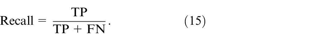
Recall

F1-score

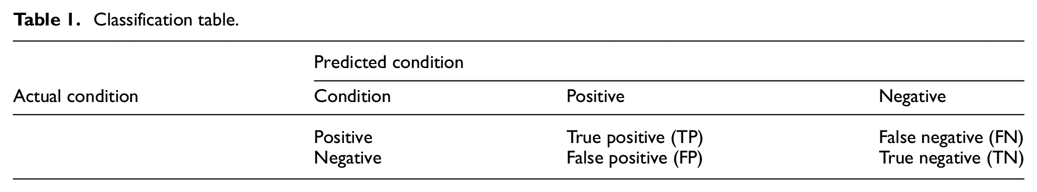
All of these measurements can be calculated according to the classification table which describes predicted and actual observed conditions (see Table 1).

Table 1.

Classification table.

	Predicted condition
Actual condition	Condition	Positive	Negative
	Positive	True positive (TP)	False negative (FN)
	Negative	False positive (FP)	True negative (TN)

Classification accuracy shows how accurately the model identifies investigated object conditions. Mathematically, accuracy can be expressed as:

\begin{matrix} Accuracy = \frac{Number of correct predictions}{Total number of predictions} \\ = \frac{TP + TN}{TP + FN + FP + TP} . \end{matrix}

(13)

Unfortunately, accuracy is an insufficient measure when experimental data are class-imbalanced.

Precision and recall are also well-known and commonly used classification accuracy metrics. Precision (or positive predictive value) shows the ratio of TP between all positively predicted conditions, while recall is the ratio of TP between all truly positive conditions:

Precision = \frac{TP}{TP + FP},

(14)

Recall = \frac{TP}{TP + FN} .

(15)

One more measure of classification accuracy, F1-score, is a so-called weighted mean of precision and recall. Also, F1-score can be treated as harmonic mean of the precision and recall and can be expressed as:

F 1 - score = \frac{2 TP}{2 TP + FP + FN} .

(16)

The F1-score is commonly used for class-imbalanced data, that is, when positive (or negative) condition ratio is significantly higher in the dataset.

Data processing

During our experiment, we have gathered the sequential data of both loaded and unloaded data as presented in Figure 3. Unfortunately, this amount of data was insufficient for model building, that is, for compilation of model training, validation, and testing sets. Under the homogeneity assumption, we developed two-step data augmentation approach for increasing the amount of experimental data. In the first data augmentation step, we divided signal into fixed-length (points $P$ ) signals of 0.2 s (80 points), 0.4 s (160 points), 0.8 s (320 points), 1.6 s (640 points), 3.2 s (1280 points), and 5.0 s (2000 points). The signal division interval was based on the principle of a sliding window:

S_{m}^{i} = [1 + i; m + i], i = 0, 1, \dots, 2000 - m,

(17)

where $S_{m}^{i}$ is $m$ -length $i$ th signal, $m$ is the fixed length of signal, $i$ is the step of signal generation. After the first data augmentation, the set of shortest signals (0.2 s) had the highest number of new signals ( $N = 384200$ ) (see Table 2).

Table 2.

Data augmentation: Number of signals after the first step and number of signals required to generate in the second augmentation step.

Signal length, s	#time points	Data augmentation
Signal length, s	#time points	Step 1	Step 2
0.2	80	384,200	0
0.4	160	368,200	16,000
0.8	320	336,200	48,000
1.6	640	272,200	112,000
3.2	1280	144,200	240,000
5.0	2000	200	384,000

Total number of signals after two steps of data augmentation were 384,200.

The second step of data augmentation was performed in order to equalize the number of signals in the sets of signals of different length. For time series data various other augmentations could be done like Hamiltonian Monte Carlo sampler³⁸ or Conditional GAN’s.³⁹ However, in order to measure the robustness of the created model, we using the noise generation techniques. The sum of two types of signal noise were used for this purpose. The first type of signal noise was a cumulative value $N_{i}$ of normally distributed random variables $N_{i} (x | μ, σ^{2})$ with mean $μ = 0$ and dispersion $σ^{2}$ in order to achieve slight drifts on signal. The second noise was a random variable of Laplace distribution in order to have small number of observations with large deviations. These signal noises are defined as follows:

U_{i} = U^{- 1} (0, 1), i = 1, 2, \dots, m,

(18)

F_{1} (x) = N_{i} (x | 0, σ^{2}) = \frac{1}{σ \sqrt{2 π}} e^{- \frac{1}{2} {(x / σ)}^{2}},

(19)

F_{2} (x) = \frac{1}{2 σ} e^{- | x | / 2 σ},

(20)

N_{i} = N_{i}^{CNorm} + N_{i}^{Lap} = (\sum_{j = 1}^{i} F_{1}^{- 1} (U_{j})) + F_{2}^{- 1} (U_{i})

(21)

here $U_{i}$ is random observations generated from uniform distribution, $σ$ is standard deviation of the distribution.

These random noises were summed up with the raw signals which were obtained from the first augmentation step. The results of data augmentation of the second step are shown in Table 2.

Results and discussion

Five models were developed for distinguishing loaded and unloaded conditions of CB: LR, SVM, RF, LSTM, and Transformer. Training and test data sets contained 80% and 20% of total separate experiments sessions to have realistic testing, respectively, for LR, SVM, and RF. For LSTM and Transformer, an additional validation data set was assigned from training set so that training, validation and test data sets contained 70% (268,940), 10% (38,420), and 20% (76,840), with same test set as for LR, SVM, and RF.

The experiments were run by using Google Colaboratory Platform, with GPU Tesla K80.

In this research, multiple configurations of all the considered models were investigated. Experimentally, the best-fitted models for our research objectives were identified. The architectures of those models are presented in Table 3. For all models, training and validation were carried out for 20 epochs with batch size of eight. The binary cross-entropy loss function was used for LSTM and Transformer.

Table 3.

Configurations of classification models.

Parameter expression
$T_{1} = \frac{1}{N} \sum_{n = 1}^{N} x_{n}$	$T_{2} = \sqrt{\frac{1}{N} \sum_{n = 1}^{N} x_{n}^{2}}$	$T_{3} = {(\frac{1}{N} \sum_{n = 1}^{N} \sqrt{\| x_{n} \|})}^{2}$	$T_{4} = \frac{1}{N} \sum_{n = 1}^{N} \| x_{n} \|$
$T_{5} = \frac{1}{N} \sum_{n = 1}^{N} (x_{n} - T_{1})^{3}$	$T_{6} = \frac{1}{N} \sum_{n = 1}^{N} (x_{n} - T_{1})^{4}$	$T_{7} = max_{n} x_{n}$	$T_{8} = min_{n} x_{n}$
$T_{9} = T_{7} - T_{8}$	$T_{10} = \frac{1}{N - 1} \sum_{n = 1}^{N} (x_{n} - T_{1})^{2}$	$T_{11} = \frac{T_{2}}{T_{4}}$	$T_{12} = \frac{T_{7}}{T_{2}}$
$T_{13} = \frac{T_{7}}{T_{4}}$	$T_{14} = \frac{T_{7}}{T_{3}}$	$T_{15} = \frac{T_{5}}{T_{2}^{3}}$	$T_{16} = \frac{T_{6}}{T_{2}^{4}}$

$N$ : signal length.

We estimated 16 parameters of time domain instead of raw signals in order to reduce the dimension of classification model input for LR, SVM, and RF models (see Table 4). Thus, all signals of 0.2 s (80 points), 0.4 s (160 points), 0.8 s (320 points), 1.6 s (640 points), 3.2 s (1280 points), and 5.0 s (2000 points) length were transformed to estimates of 16 parameters. Such a signal transformation allowed highlighting predominant features of the classes and allowed interpreting the results of LR, SVM, and RF models more accurately. Since deep neural network?/model? can obtain better generalization from raw data, we used raw signal data for both LSTM and Transformer neural networks.

Table 4.

Statistical parameters LR, SVM, and RF models.

Model	Architecture/hyper-parameters
LR	no hyper-parameters
SVM	regularization parameter-1.0, kernel-radial basis function, degree of the polynomial − 3,
RF	number of trees in RF-100, supported criteria-Gini, maximum depth of the tree-8 bootstrap used
LSTM*	LSTM → dropout → LSTM → linear → sigmoid
Transformer *	four sequential blocks:
	normalization → multi head attention
	dropout → normalization
	1D convolution → dropout →
	1D convolution →
	concatenation
	multilayer perceptron:
	global average pooling →
	linear → dropout →
	linear → sigmoid

Number of LSTM model hyper-parameters was 70,953. Transformer model hyper-parameters variated from 17,033 to 78,473 for 0.2 and 5.0 s-length signal models, respectively.

Aggregated signal classification models

Training time for models LR, SVM, and RF did not depend on signal length because the number of model input parameters was always stable and equal to 16. LR model was able to perform the training in the fastest way in ~4 s. RF and SVM models were much slower; their training session took ~86 s and even ~10,000 s, respectively.

The results that we present further are based on independent test data which was generated during independent experiment session. Testing of the models showed that the accuracy of the model classification increases monotonically as the input signal lengthens (see Table 5) with models used aggregated signal statistics. In LR, SVM, and RF models the accuracy of the model increased by 4% on the average each time when the signal length was doubled. RF was the most accurate among the three models and was able to classify 3.2 and 5.0 s-length signals with an accuracy of 79% and 78%, which was by 3% higher than that of LR or SVM. It is worth to pay attention that RF was the most accurate in classifying the signals of all lengths. Only 0.4 s length signal classification accuracy was the same in RF as in SVM. In general, the accuracy of the models satisfied the inequality:

accurac y_{L R} \leq accurac y_{S VM} \leq accurac y_{R F}

(22)

Table 5.

Classification metrics for all models.

Model		Signal length, s
Model		0.2	0.4	0.8	1.6	3.2	5.0
Accuracy, %
LR		57	61	65	69	72	76
SVM		58	62	66	71	74	76
RF		60	62	67	74	79	78
Transformer		60	63	69	81	92	100
LSTM		72	77	98	100	100	100
Precision
LR	Unloaded	47	51	56	60	64	70
	Loaded	68	71	73	76	78	81
SVM	Unloaded	48	52	56	64	67	69
	Loaded	69	70	73	76	79	81
RF	Unloaded	50	51	57	66	75	78
	Loaded	71	72	78	79	82	78
Transformer	Unloaded	50	54	60	73	88	100
	Loaded	68	70	76	87	96	100
LSTM	Unloaded	60	65	97	100	100	100
	Loaded	88	92	98	100	100	100
Recall
LR	Unloaded	64	63	63	66	69	72
	Loaded	68	60	67	71	75	79
SVM	Unloaded	64	59	63	64	69	72
	Loaded	65	64	68	77	78	79
RF	Unloaded	66	67	74	70	72	63
	Loaded	56	58	52	76	84	88
Transformer	Unloaded	55	58	67	81	94	100
	Loaded	63	67	70	80	92	100
LSTM	Unloaded	87	92	98	100	100	100
	Loaded	62	68	98	100	100	100
F1-score
LR	Unloaded	54	56	59	63	67	71
	Loaded	59	65	70	73	76	80
SVM	Unloaded	55	56	59	64	68	71
	Loaded	61	67	70	76	78	80
RF	Unloaded	57	58	64	68	73	70
	Loaded	63	64	69	77	83	83
Transformer	Unloaded	53	56	63	77	91	100
	Loaded	65	69	73	83	94	100
LSTM	Unloaded	71	76	98	100	100	100
	Loaded	72	78	98	100	100	100

for all length signals.

Precision of the models in classifying CB without load increased significantly faster with increasing signal length: precision of LR, SVM, and RF increased from the shortest to the longest signal by 23% and 13%, by 21% and 12%, by 28% and 7% for unloaded and loaded CB condition, respectively. Since 0.2 s is equivalent to the length of one peak cycle, this fact shows that the models were able to identify more accurately the unloaded signals as they lengthened what confirms the assumption that numerical characteristics of short signals of loaded and unloaded CB are very similar and only individual signal peaks stand out for their numerical characteristics. It follows that the models, combining the peaks into longer peak circuits, are able to classify the signals more accurately with less fluctuating numerical characteristics.

In all three models using aggregated signals, the highest recall was observed for classification of a loaded condition. Recall of the loaded condition classification has been considerably increasing with the signal elongation: LR, SVM, and RF models’ recall of loaded CB classification increased by 11%, 14%, and even 32%, respectively, while unloaded classification recall increased by 8%, 8%, and 6% for LR, SVM, and RF, respectively. Recall results show that by increasing signal length higher number of signals represented loaded CB condition can be correctly classified, while they were incorrectly classified as unloaded with shorter signal length. In this way, recall support the assumption that the signal peaks obtained from the CB under load are more characteristic, whereas rotating empty CBs generate signal peaks of different spectra, which are often incorrectly assigned to the load class and the models can classify unloaded CB more sensitively only by combining the peaks into longer sequences.

The F1-score summarizes the results of precision and recall tests. F1-score reflects the accuracy of the classification of models with imbalanced data better than the accuracy measure, therefore it can be argued that the models LR, SVM, and RF classify different CB conditions almost identically.

The latter analysis allows concluding that all classification models of aggregated signals gave similar classification results. Noteworthy, SVM model took unacceptably long time to train the model and due to this reason SVM is not suitable for solving this type of classification tasks. Meanwhile, although the classification statistics were almost identical for LR and RF, RF showed slightly higher accuracy and F1-score. However, the training time of LR was 21.5 times shorter than that of RF (4 and 86 s, respectively).

Raw signal classification models

LSTM and Transformer models were developed to classify raw CB signals. Each model was trained with signals of different lengths (0.2, 0.4, 0.8, 1.6, 3.2, and 5.0 s) by repeating the training for 20 epochs.

Training time for LSTM and Transformer models was strongly dependent on the length of the signal. The shortest signals of 0.2 s trained faster and the training for one epoch interfered with 343 s for LSTM and 410 s for Transformer using GPU memory. Meanwhile, models with the longest 5.0 s length signal also took the longest time to be trained and its training for one epoch interfered with 4600 s for LSTM and 14,800 s for Transformer using GPU memory, which took 17.5 and 36.1 times longer than training for 0.2 s signal, respectively (see Table 6).

Table 6.

Time required to train one epoch for LSTM and transformer models using raw signal.

Signal length, s	#time points	One epoch training time, s
Signal length, s	#time points	LSTM	Transformer
0.2	80	343	410
0.4	160	510	450
0.8	320	830	750
1.6	640	1550	1950
3.2	1280	2850	6460
5.0	2000	4600	14,800

Classification metrics of the models are shown in Table 5. The accuracy of LSTM and Transformer models increased very rapidly with increasing signal length and an accuracy of 100% was achieved when using both models with the longest signals. The accuracy of Transformer increased on average by 8% when doubling the signal length and after training with the longest signal of 5.0 s, its accuracy reached 100%. The accuracy of LSTM model grew even faster and after training with the 1.6 s signal, the accuracy reached 100%. In the case of Transformer, a monotonically constant increase in accuracy was observed with the elongation of the signal, but in the case of LSTM the accuracy of the model increased by 5%, and doubling the signal length up to 0.8 s led to increase in accuracy by 21% points up to 98%.

Comparative analysis of the precision of the models shows that LSTM classified the loaded CB even by 20% points more precisely than Transformer and reached 88$ with the shortest (0.2 s) signal. Transformer’s precision with the same-length signal reached 63% only. However, as in the case of classification of aggregated signals, both models classified the loaded CB much more precisely than the idle CB when using short signals. Nevertheless, both models achieved a precision of 100% when classifying both CB states: Transformer achieved this level of accuracy with 5.0 s-length signal and LSTM with 1.6 s-length signal.

The sensitivity of the models demonstrated some noteworthy aspects. Transformer, like other models (LR, SVM, and RF), classified loaded CBs more sensitively when using short signals than when using the longer ones. However, starting from 1.6 s-length signal Transformer’s sensitivity of classifying unloaded CB condition jumped significantly by 23% and reached 85%, while the sensitivity of loaded CB classification increased by only 5% and reached 79% for this length of the signal, that is, the model has started to classify the idle CB state more sensitively. In the case of LSTM model, the sensitivity to classify the unloaded CB condition using the shortest signal is significantly higher than that of the loaded CB (87% vs 62%, respectively), but starting from 0.8 s-length signal, the sensitivity started to be same for both CB conditions, and starting from 1.6 s-length signal, the sensitivity reached 100%.

The F1-score, which is more suitable to measure the accuracy of classification of imbalanced data, showed that LSTM model was the optimal one and was able to classify both CB states with equal accuracy for all lengths of signal. Meanwhile Transformer performed in exactly the same way as LR, SVM, or RF, that is, it classified the state of loaded CB more accurately than that of a idle CB regardless of signal length.

Summarizing our analysis of raw signal classification models, LSTM model demonstrated clear advantages in terms of both shorter training time and significantly better classification accuracy measurements.

Investigation of model robustness

We chose LSTM model with signal length of 1.6 s for evaluation of sensitivity of correct classification of CB conditions. Beginning with the first step of augmentation, we used 1.6 s-length signals as the set for the test of robustness assessment. Three types of noise (see equation (21)) were added to the signals:

Random Laplace noise $N^{Lap}$ . The errors of this type are caused by unpredictable fluctuations in signal reading and are not dependent on the deterioration of CB or the qualification of the experimenter. Random Laplace noise have small number of large deviations.

Drifted noise $N^{CNorm}$ . It cumulative error which can appear due to either the flaws of the measurement system, the deterioration of CB or poor qualification of the experimenter. Drifted noise is a cumulative value of normally distributed random variable.

Noise $N$ . It is a sum of random and drifted noise.

Eleven different noise levels were selected for evaluation of the sensitivity of the model. The signal with the highest noise was generated by adding the noise depending on the standard variation of the raw signal to the raw signal. The signal noise was further reduced by reducing the standard deviation by $10, 20, \dots, 100$ times (see Figure 5(a)–(c)).

Figure 5.

Signals with noise: (a) random Laplace noise $N^{Lap}$ , (b) drifted noise $N^{CNorm}$ , and (c) noise $N = N^{Lap} + N^{CNorm}$ .

Classification of signals with different types and levels of noise showed that the model was the least sensitive to the random element-wise Laplace noise. The random noise had almost no effect on the accuracy of the model until the noise reached 20-times lower value of the standard deviation, that is, only at extremely high noises $> std \times 10^{- 1}$ (see Figure 6). However, the biased noise had a much greater effect on the accuracy of the model, although under relatively large standard deviation the model was able to classify with the accuracy of >90%. Figure 6 shows that the biased noise was considerably more significant than the random noise and had higher effect at all noise levels.

Figure 6.

LSTM model classification accuracy when the signals of different noise type and level are classified.

Conclusion

In this article, the investigation of ML methods to classify CB load is presented. We have introduced CORBEL dataset and developed five ML models (LR, SVM, RF, LSTM, and Transformer) for distinguishing loaded and unloaded conditions of CB. The objective of this research was reached by working out the algorithm able to identify 100% and distinguish loads placed on the belt conveyor. The proposed LSTM and Transformer models were able to classify signals precisely with accuracy, precision, recall, and F1-score of 100%. Shallow models such as LR, SVM, and RF performed considerably worse in classification of different CB conditions. The final and the best-performing model is based on LSTM and can successfully classify CB condition starting even from 1.6 s-signal, while other models reach their best performance with the longest (5.0 s) signal only. The proposed LSTM and Transformer models solve the problem of signal classification by using raw signal information. Our experiments prove that class-weighting in addressing class imbalance can improve the model performance. Moreover, final model can be trained relatively quickly and have short inference time, therefore it can be meaningfully employed for practical use. Promising results of this paper indicate the feasibility of the model for identification of loaded states of the belt in real-time mode. In our future research, we plan to perform different tests on various failures and malfunctions. Finally, we have made available to the public the code of the proposed network architectures, our research data and the interface for CB classification. The repository can be found online at GitHub https://github.com/TadasZvirblis/CORBEL.

Footnotes

Acknowledgements

The authors would like to thank Google LLC for supplying computational resources for this study via Google Colaboratory Platform (abbr. Colab).

Handling Editor: Chenhui Liang

Declaration of conflicting interests

The author(s) declared no potential conflicts of interest with respect to the research, authorship, and/or publication of this article.

Funding

The author(s) received no financial support for the research, authorship, and/or publication of this article.

ORCID iDs

Tadas Žvirblis

Linas Petkevičius

References

Rybicka

Caban

The use of a plate conveyor for transporting aluminum cans in the food industry. Adv Sci Technol Res J 2020; 14: 26–31.

Mazurkiewicz

Maintenance of belt conveyors using an expert system based on fuzzy logic. Arch Civil Mech Eng 2015; 15: 412–418.

Błażej

Jurdziak

Kawalec

. Condition monitoring of conveyor belts as a tool for proper selection of their replacement time. In: International conference on condition monitoring of machinery in non-stationary operation, Lyon, France, 15–16 December2014, pp.483–494. Springer.

Fedorko

Molnár

Michalik

, et al. Failure analysis of conveyor belt samples under tensile load. J Ind Text 2019; 48: 1364–1383.

Napoleone

Macchi

Pozzetti

A review on the characteristics of cyber-physical systems for the future smart factories. J Manuf Syst 2020; 54: 305–335.

Zhang

Smart factory reference architecture based on cps fractal. IFAC-PapersOnLine 2019; 52: 2776–2781.

Mörth

Emmanouilidis

Hafner

, et al. Cyber-physical systems for performance monitoring in production intralogistics. Comput Ind Eng 2020; 142: 106333.

Fedorko

Application possibilities of virtual reality in failure analysis of conveyor belts. Eng Fail Anal 2021; 128: 105615.

Andrejiova

Grincova

Marasova

Identification with machine learning techniques of a classification model for the degree of damage to rubber-textile conveyor belts with the aim to achieve sustainability. Eng Fail Anal 2021; 127: 105564.

10.

Wodecki

Zdunek

Wyłomańska

, et al. Nonnegative factorization of spectrogram for local damage detection of belt conveyor gearboxes. IFAC-PapersOnLine 2017; 50: 4714–4718.

11.

Andrejiova

Grincova

Classification of impact damage on a rubber-textile conveyor belt using naïve-bayes methodology. Wear 2018; 414–415: 59–67.

12.

Andrejiova

Grincova

Marasova

Failure analysis of the rubber-textile conveyor belts using classification models. Eng Fail Anal 2019; 101: 407–417.

13.

Yang

Zhou

Song

Audio-based fault diagnosis for belt conveyor rollers. Neurocomputing 2020; 397: 447–456.

14.

Bortnowski

Nowak-Szpak

Ozdoba

, et al. The acoustic camera as a tool to identify belt conveyor noises. J Sustain Min 2021; 19: 286–294.

15.

Hou

Qiao

Zhang

, et al. Multispectral visual detection method for conveyor belt longitudinal tear. Measurement 2019; 143: 246–257.

16.

Grzesiek

Zimroz

Śliwiński

, et al. Long term belt conveyor gearbox temperature data analysis – statistical tests for anomaly detection. Measurement 2020; 165: 108124.

17.

Błażej

Jurdziak

Kozłowski

, et al. The use of magnetic sensors in monitoring the condition of the core in steel cord conveyor belts – tests of the measuring probe and the design of the diagbelt system. Measurement 2018; 123: 48–53.

18.

Dariusz

Computer-aided maintenance and reliability management systems for conveyor belts. Eksploatacja i Niezawodnosc 2014; 16: 377–382.

19.

Fedorko

Molnar

Marasova

, et al. Failure analysis of belt conveyor damage caused by the falling material. Part ii: Application of computer metrotomography. Eng Fail Anal 2013; 34: 431–442.

20.

Liu

Miao

, et al. Research on the fault analysis method of belt conveyor idlers based on sound and thermal infrared image features. Measurement 2021; 186: 110177.

21.

Che

Qiao

Yang

, et al. Longitudinal tear detection method of conveyor belt based on audio-visual fusion. Measurement 2021; 176: 109152.

22.

Santos

Rocha

FAS

Reis

AJDR

, et al. Automatic system for visual detection of dirt buildup on conveyor belts using convolutional neural networks. Sensors 2020; 20: 5762.

23.

Zhang

Shi

Zhang

, et al. Deep learning-based damage detection of mining conveyor belt. Measurement 2021; 175: 109130.

24.

Zhao

Typical failure analysis and processing of belt conveyor. Procedia Eng 2011; 26: 942–946.

25.

Kobayashi

Toya

Effect of belt transport speed and other factors on belt mistracking. Microsyst Technol 2007; 13: 1325–1330.

26.

Ryba

Initial tests of the rubber belts tension of conveyors with a prototype measuring system. Mechanik 2021; 1: 20–22.

27.

Bzinkowski

Ryba

Siemiatkowski

, et al. Real-time monitoring of the rubber belt tension in an industrial conveyor. Rep Mech Eng 2022; 3: 1–10.

28.

Ryba

Rucki

Siemiatkowski

, et al. Design and calibration of the system supervising belt tension and wear in an industrial feeder. Facta Universitatis Series Mechanical Engineering 2022; 20: 167–176.

29.

David

Mitchel

Erica Rihl

Logistic regression: a self-learning text. New York, NY: Springer, 2002.

30.

Cervantes

Garcia-Lamont

Rodríguez-Mazahua

, et al. A comprehensive survey on support vector machine classification: applications, challenges and trends. Neurocomputing 2020; 408: 189–215.

31.

Breiman

Random forests. Mach Learn 2001; 45: 5–32.

32.

Ian

Yoshua

Aaron

Deep learning. Cambridge, MA: MIT Press, 2016.

33.

Hochreiter

Schmidhuber

Long short-term memory. Neural Comput 1997; 9: 1735–1780.

34.

Ashish

Noam

Niki

, et al. Attention is all you need. Adv Neural Inf Process Syst 2017; 30: 1–15.

35.

Alec

Jeffrey

Rewon

, et al. Language models are unsupervised multitask learners. OpenAI blog 2019; 1: 9.

36.

Dong

. Speech-transformer: a no-recurrence sequence-to-sequence model for speech recognition. In: 2018 IEEE international conference on acoustics, speech and signal processing (ICASSP), April 2018, pp.5884–5888. New York, NY: IEEE.

37.

Shiyang

Xiaoyong

Yao

, et al. Enhancing the locality and breaking the memory bottleneck of transformer on time series forecasting. Adv Neural Inf Process Syst 2019; 32: 5243–5253.

38.

Bou-Rabee

Sanz-Serna

JM.

Randomized Hamiltonian Monte Carlo. Ann Appl Probab 2017; 27: 2159–2194.

39.

Smith

Conditional GAN for timeseries generation. arXiv preprint arXiv:2006.16477, 2020.

Investigation of deep learning models on identification of minimum signal length for precise classification of conveyor rubber belt loads

Abstract

Keywords

Introduction

Methodology and data description

CB-monitoring system concept and calibration issue

Data acquisition

Machine learning methods

Logistic regression

Support vector machine

Random forest

Long short-term memory

Transformer neural network

Classification accuracy metrics

Data processing

Results and discussion

Aggregated signal classification models

Raw signal classification models

Investigation of model robustness

Conclusion

Footnotes

Acknowledgements

Declaration of conflicting interests

Funding

ORCID iDs

References