Sage Journals: Discover world-class research

Abstract

Hollow ball screws play a vital role in high-quality precision manufacturing, in which sensors are used to obtain useful data. The use of artificial intelligence to determine the condition of machines is a major trend, and installing multiple sensors on relevant objects may be prohibitively expensive. This study compares a machine learning method based on a support vector machine (SVM) with deep learning methods. In the machine learning strategy, built-in signals from internal parameters are used to determine the condition of the hollow ball screw. Rather than using a graphics processing unit (GPU), feature engineering and then Fisher’s score were applied to determine the most representative parameters from fusion sensor signals to perform SVM classification. For the deep learning method, a GPU was employed instead of data cleaning; a long- and short-term memory (LSTM) network and hybrid convolutional neural network (CNN) and an LSTM network were used to automatically extract effective features and then perform classification. Thus, the deep learning approach enabled classification of one-dimensional (1D) and multidimensional data sets, through which users can obtain suitable configurations for various sensors according to cost and other requirements for classification accuracy. We compared the accuracies of the LSTM, CNN–LSTM, and SVM models by using multiple datasets. The 3D LSTM model with current, rpm, and additional linear scale signals provided good synergy for feature extraction and resulted in the maximum accuracy close to the highest accuracy of the supervised fine-tuned SVM model by using current signal. Datasets that are unrepresentative according to FE analysis may be useful in deep learning. The advantages of using a deep learning model without feature extraction relative to those of SVM learning was investigated.

Keywords

Hollow ball screw support vector machine convolutional neural network long- and short-term memory hybrid neural network

Introduction

The hollow ball screw is a transmission element that converts rotary motion into linear motion in manufacturing processes. The pretightening force of the ball screw results in thermal deformation following its continual motion. When this pretightening force is lost, the accuracy of the ball screw position is affected. Wei et al.¹ analyzed ball screw mechanical characteristics, such as the contact angle and the coefficient of friction between the ball nut and the ball screw. The Hilbert–Huang transform has also been applied to processing and research on ball screw failure and mechanical signals.^2,3 The pretension of the ball screw in a feed drive system improves its mechanical strength and maintains a minimum rigidity. However, the continual movement of the ball screw subjects it to thermal deformation, which results in positioning errors in the feed system and reduces the overall positioning accuracy. In addition, the ball screw generates pretension when it is subjected to thermal deformation; although this can be compensated for, a controller cannot display the previous positioning error. Therefore, studying the prediction of ball screw positioning errors and developing online compensation methods are essential.^4,5

Conventional maintenance tasks include breakdown maintenance, scheduled preventive maintenance, and condition-based maintenance (CBM). In CBM, experts monitor the health of a sensorless machine on the basis of variables such as the driving voltage and current, which are obtained by attaching sensors, such as accelerometers and microphones, at key positions or locations. Next, by combining these data with knowledge about the machine, experts can determine its health. Systematic, data-driven methods have been used to trace the causes of major problems that occur in the ball screws of feed drive systems or computer numerical control (CNC) machines in manufacturing processes. In such studies, the failure signatures have been identified and classified using various prediction models. Currently, artificial intelligence is increasingly applied to the maintenance, monitoring, and health determination of various production-line machines. Wang and Vachtsevanos⁶ applied a cyclic wavelet neural network to diagnose and forecast the breakdown of rolling components. Tsai et al.⁷ proposed an angular velocity Vold–Kalman order tracking filter to monitor changes in the passing frequency of a ball screw for the detection of any pretension loss. However, among fault diagnosis algorithms, support vector machines (SVMs) are commonly applied because they have a short training time and minimal training data requirements while still achieving highly effective classification of various features.⁸ Huang and Zheng⁹ investigated the ball screw preload problems by applying different ball nut preloads. Through the ball screw feed drive motion, the irregular change of current and the rolling ball vibration signals of the ball screw can be distinguished by SVM.

Wang et al.¹⁰ proposed an ensemble SVM to classify blur images into four types; moreover, they compared the standard SVM with other blur classification methods to demonstrate ensemble SVM superior performance. Patel and Upadhyay¹¹ compared SVM and artificial neural network (ANN) methods for the identification of ball bearing faults. However, ANN training is a challenging task. Several shortcomings of ANN classification are listed as follows:

ANNs train using gradient descent optimization, and they are black box models with many parameters. Therefore, the classification speed of ANNs is slow.

ANNs are often subject to overfitting due to insufficient or irrelevant training data.

The Vapnik–Chervonenkis (VC) dimension for ANN-based classification remains poorly understood.¹²

Studies have demonstrated that when the number of training samples is limited, the classification accuracy of SVMs is typically higher than that of ANNs. However, the SVM algorithm has no standard method for the selection of the parameters of the kernel functions or the parameters for the loss function.¹³ In addition, for SVMs, each classification problem is associated with an optimal parameter set. However, if the features of the training data are not clearly distinguished, then the accuracy of the SVM results will be reduced. To solve these problems, we developed an architecture for feature engineering based on data mining that increases the dimensionality of the raw data. We then expanded the data set by selecting the optimal combination of features.

Compared with conventional ANNs, deep ANNs have a higher number of hidden layers. When employing complex nonlinear models with large data sets, the hidden layers hidden in deep ANNs enable the model to accurately learn complex relationships between inputs and outputs. Ho et al.¹⁴ the convolutional neural networks (CNN) and traditional rule-based systems was also used for the automatic optical inspection for silicone rubber gaskets.

Long short-term memory (LSTM) is a type of deep learning architecture. Hochreiter and Jürgen¹⁵ developed the LSTM model by building on deep recurrent neural networks (RNNs); the LSTM model enables previous weights to be retained through the use of hidden layers. The LSTM model built on the RNN architecture by including the upper and lower signals from previous time steps. In particular, the LSTM model can predict time series signals, learn complex nonlinear models, and perform automatic feature extraction; thus, it is very suitable for time series data. Time series models usually employ a past observation lag to predict a future status. Therefore, when a time series model is being used to make predictions, the choice of an appropriate lag is highly important.¹⁶ This increases the accuracy of model predictions and facilitates understanding of the data generation.

However, conventional data-driven models are increasingly unable to meet the high requirements for forecast accuracy, and many methods for processing complex data have been introduced.¹⁷ To enhance the performance of Remaining useful life (RUL) prediction, a series of deep learning models have been developed with automatic feature extraction and high-accuracy prediction.¹⁸ In the field of RUL prediction, CNNs have been employed to obtain high-level spatial features from raw sensor signals,^19,20 and LSTM networks have been used to extract signals from a specific sensor.^21–24

However, these deep learning models have included either spatial or temporal signal characteristics. Therefore, recent studies^25–29 have proposed combining CNN and LSTM models. Most such studies have focused on natural language processing, video processing, and speech processing. The prediction set of a CNN–LSTM model is countable,³⁰ and raw sensor signals can be used to directly predict residential energy consumption.³¹

In the present study, a three-stage method was proposed for fault identification. In the first stage, let the single-axis ball screw travel back and forth for 5, 30, and 60 min; we then collected the motor current signal, screw rotation signal, and position signal using an optical ruler. Fisher’s score was applied to these data to determine which was most suitable for fault identification. During the second stage, we designed a process similar to the actual factory processing path to reduce the machine preheating time. In the final stage, conventional machine learning and deep learning methods were applied for classification with the same data set. A GPU was not used for the conventional machine learning methods, and Fisher’s score was used to determine the most suitable features in the fusion sensor signals for SVM classification. For the deep learning methods, a GPU was used to replace feature engineering, and we employed LSTM and CNN–LSTM models to perform automatic feature extraction prior to classification. The developed models were applicable to one-dimensional or multidimensional data sets, and their classification outputs enabled users to determine the appropriate configurations for various cost and accuracy requirements. Testing the LSTM, CNN–LSTM, and SVM models with multiple data sets revealed that the SVM model yielded the highest accuracy, followed by the LSTM model.

Methods

Support vector machines

Vapnik^32,33 developed the first linear classifier SVM to distinguish various categories. This original SVM solved binary classification problems by searching for the optimal hyperplane separating the data categories. In a simple binary classification problem, such as that shown in Figure 1, with a wide margin, the hyperplane can separate the data without errors. The mathematical model of the SVM is presented as follows.

Figure 1.

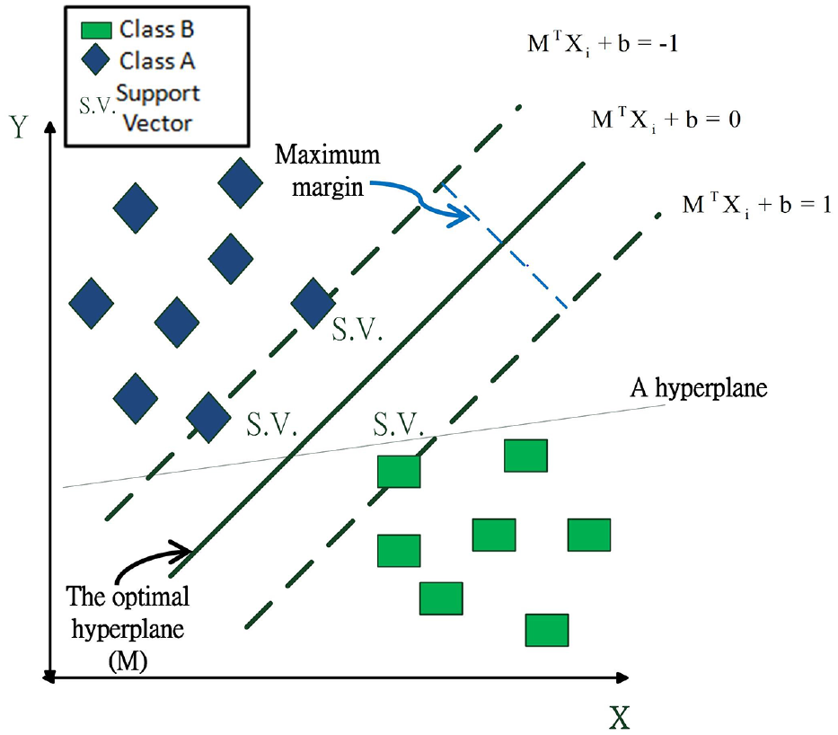
Diagram of SVM classification with a linearly separable data set.

A binary classification problem is defined for a valid set of points $X_{i}$ (i = 1, 2, …, n), where each point is classified as A or B, with labels $\forall_{i} = \pm 1$ . Equation (1) can satisfy the data points of the binary classification problem with $y_{i} (M^{T} X_{i} + b) \geq 0 \forall_{i}$ , where $M^{T}$ is the vector set of the optimal hyperplane and b is the bias.

y_{i} (M^{T} X_{i} + b) \geq 0 \forall_{i}

(1)

The goal of the SVM is to determine the optimal hyperplane with the widest margin. This optimization problem is represented by equations (2) and (3), which are the models that define a hard-edged SVM.

\min, Φ (M) = \frac{1}{2} M^{2}

(2)

Subject to, y_{i} (M^{T} X_{i} + b) \geq 1, i = 1, 2, \dots, n

(3)

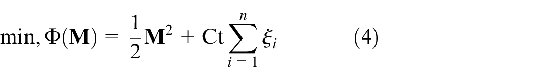
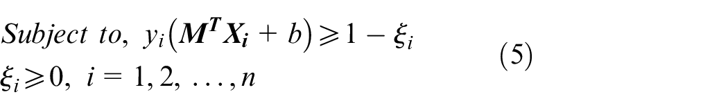
Most real-world classification problems are nonlinear and contain outliers, which presents challenges for classification and causes errors. Therefore, equations (4) and (5) are models for a soft margin SVM, where $ξ_{i}$ is the introduced loose variable and the entire data set has a tolerance range for misclassification. Each diagnostic point corresponds to the value of its loose variable. The cost parameter $Ct$ influences the maximum margin and the user can determine the influence of the loose variable.

\min, Φ (M) = \frac{1}{2} M^{2} + Ct \sum_{i = 1}^{n} ξ_{i}

(4)

\begin{matrix} Subject to, y_{i} (M^{T} X_{i} + b) \geq 1 - ξ_{i} \\ ξ_{i} \geq 0, i = 1, 2, \dots, n \end{matrix}

(5)

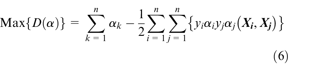
To reduce the complexity of equations (4) and (5), they can be transformed into equivalent dual problems, such as equations (6) and (7), by using a Lagrange transformation

Max {D (α)} = \sum_{k = 1}^{n} α_{k} - \frac{1}{2} \sum_{i = 1}^{n} \sum_{j = 1}^{n} {y_{i} α_{i} y_{j} α_{j} (X_{i}, X_{j})}

(6)

constraint : \sum_{j = 1}^{n} y_{j} α_{j} = 0 and C \geq α_{i} \geq 0, i = 1, 2, \dots, n

(7)

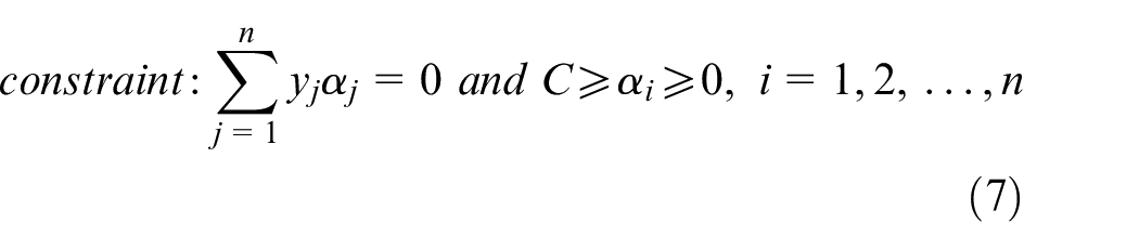
where $(X_{i}, X_{j})$ represents the inner product of $X_{i}$ and $X_{j}$ , $α$ is the Lagrangian multiplier, and the objective is to maximize ${D (α)}$ under the constraints defined in equation (7).

Feature engineering

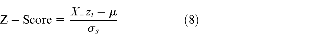
The original signals received by sensors are processed, in Data segmentation step, the data are split into a fixed number of segments. In Select torque or stationary section step, data within a limit of six standard deviations can then be filtered to obtain the torque or the fixed part of the signal; in Feature extraction step, feature extraction is performed. First, the original time-domain data are transformed into power spectral density–amplitude (PSD-Amp) and PSD-Shape in the frequency domain. Second, statistical features are extracted from the time and frequency domains. In remove outliers step, the Z-score is used to identify outliers for each feature; these outliers are removed to prevent them from interfering with the algorithm training. The Z-score formula is presented in equation (8).

Z - Score = \frac{X_z_{i} - μ}{σ_{s}}

(8)

$X_z_{i}$ stands for the ith section in the feature, µ expresses the mean of the feature, and $σ_{s}$ is the standard deviation of the feature.

In Feature Selection step, Fisher’s score³⁴ is used to pick out the most distinctive features. Criteria. The formula is shown in equation (9).

FS = \frac{{(m_{2 -} m_{1})}^{2}}{s_{1}^{2} + s_{2}^{2}}

(9)

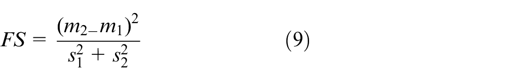
m expresses the mean of the class feature and s is the standard deviation of the class feature. The score derived from Fisher’s criteria is an index of the degree of distinction. In normalization step, the data are normalized to reduce computational complexity and facilitate classification.^35–38 The steps for feature engineering are illustrated in Figure 2.

Figure 2.

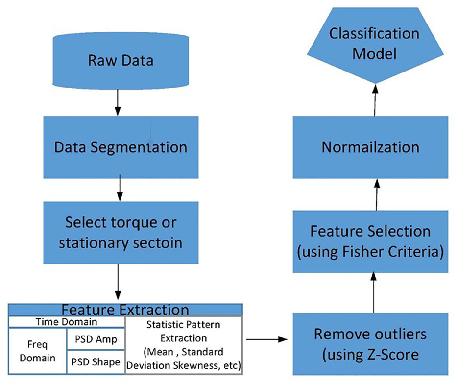
Feature engineering flow chart.³⁸

Convolutional neural network

CNNs are potentially suitable for processing sensor measurement data and extracting high-level spatial features. CNN architectures typically comprise a convolutional layer, a pooling layer, a fully connected (FC) layer with dropout, and a softmax layer for classification (Figure 3). In the convolutional layer, convolutional filters are used to extract features from the input, which thus performs feature extraction and feature mapping. An activation function is then applied to obtain the feature map for the next layer. The output of the convolution filter is calculated using the following formula:

z^{l} = w^{l} * c l^{l - 1} + b^{l},

(10)

c l^{l} = ac (z^{l})

(11)

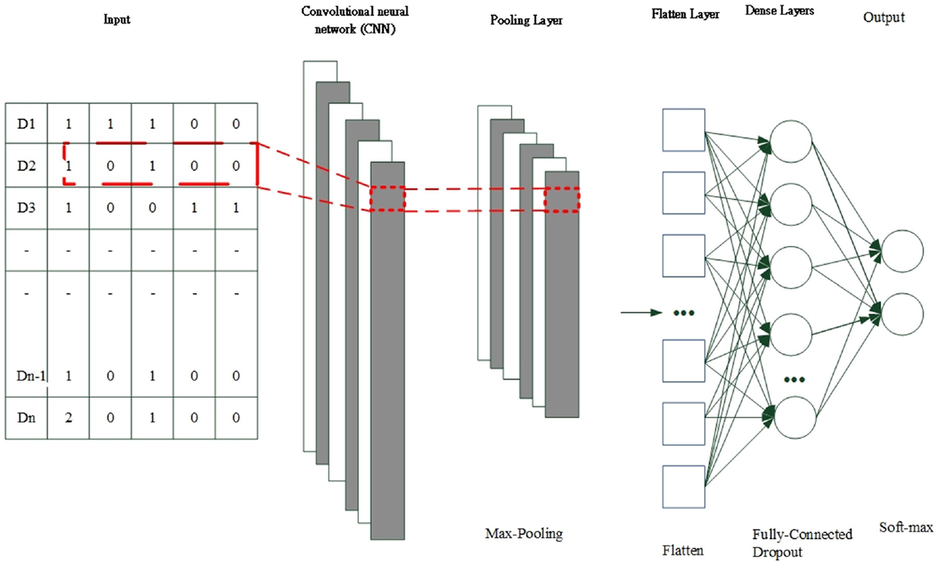
where * denotes the convolutional operation, $l$ is the layer number in the network, and $c l^{l - 1}$ and $c l^{l}$ are the input and output of the convolution filter, respectively. Moreover, $ac (.)$ is the activation function, $z^{l}$ is the input of the activation function, $w^{l}$ is the weight matrix of the convolutional filter, and $b^{l}$ is the additive bias vector.

Figure 3.

CNN architecture.

In the pooling layer, the output of the convolutional layer is downsampled by an appropriate factor to reduce the resolution of the feature map. Average pooling and maximum pooling are the most common methods, and maximum pooling is used herein. The formula for maximum pooling is given as follows:

c l^{l} = down (c l^{l})

(12)

where $down (\cdot)$ represents the downsample function for maximum pooling.

FC layers with dropout are used to aid training in deep neural networks. For each training batch, half of the feature detectors are ignored, which substantially reduces overfitting. This method reduces the interaction between feature detectors, without which some detectors rely on other detectors to function.

When the softmax operation is applied, the sum of the probability distributions of the final layer outputs is equal to 1. For example, consider a classification with two categories. The input is a signal image, and the output softmax activation function returns the probability of the image belonging to the two categories. The sum of these probabilities is 1.

S (fl)_{i} = \frac{e^{f l_{i}}}{\sum_{j = 1}^{Cs} e^{f l_{j}}}

(13)

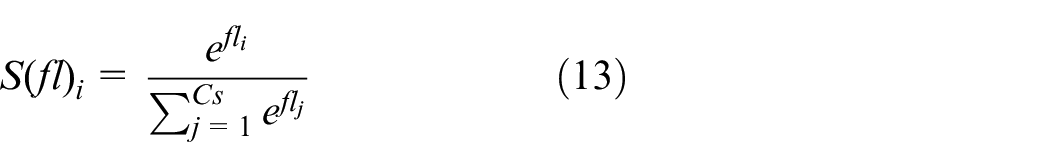
In equation (13), $S (fl)_{i}$ is in the range (0, 1), which is required for this value to be a probability. The $fl$ input vector for the softmax function is given as ( $f l_{1}$ , …, $f l_{c}$ ), with elements $f l_{i}$ . The standard exponential function is applied to each element of the input vector. Division by $\sum_{j = 1}^{Cs} e^{f l_{j}}$ ensures that the sum of the softmax output values is 1; this term is the normalization term. $Cs$ is the number of classes in the multiclass classifier.

RNN and LSTM-RNN

RNNs are special ANNs with a directional connection between the units in a single layer. This makes them suitable for sequential data. RNNs are called loops because RNNs perform the same task for each element in a sequence. RNNs also have memory because the current output state depends on previous calculations. However, because of the vanishing gradient problem, RNNs are only suitable for a limited number of time steps. An unfolded view of the RNN configuration is shown in Figure 4.³⁹

Figure 4.

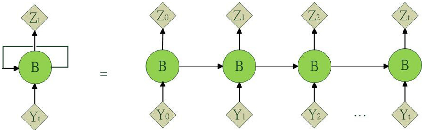
RNN and its unfolded view.

Standard RNNs are subject to the vanishing and exploding gradient problems, and the LSTM architecture was specially designed to overcome these problems. Gates are introduced in this model to control the gradient flow and retain long-term dependencies. The key components of the LSTM architecture are the memory cell and gates, as shown in Figure 5.³⁹

Figure 5.

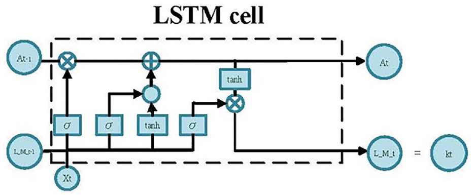
Information flow in the LSTM block of an RNN.

The gates in the LSTM block enable it to retain a more constant error, which can be backpropagated through time and layers. This improves the ability of the RNN to learn over many time steps.⁴⁰ The gates work together store information related to long-term and short-term sequences. RNNs use recursion to model the input sequence {x1, x2, …, xn} as follows:

L_M_{t} = g (L_M_{t - 1}, X_{t})

(14)

where $Xt$ is the input at time t and $L_M_{t}$ is the hidden state at time t. The gate is introduced using the recursive function g to solve the problems of vanishing or exploding gradients. The state of the LSTM unit is calculated as follows:

i g_{t} = σ (w_{i} [L_M_{t - 1}, X_{t}] + b_{i}

(15)

f g_{t} = σ (w_{f} [L_M_{t - 1}, X_{t}] + b_{f}

(16)

o g_{t} = σ (w_{o} [L_M_{t - 1}, X_{t}] + b_{o})

(17)

A_{t} = f g_{t} ⊙ A_{t - 1} + i g_{t} ⊙ {\tilde{A}}_{t}

(18)

\tilde{A} = thah (w_{c} [L_M_{t - 1}, X_{t}] + b_{c})

(19)

L_M_{t} = o g_{t} ⊙ \tanh (A_{t})

(20)

where $i g_{t}$ , $f g_{t}$ , and $o g_{t}$ are input, forget, and output gates, respectively; w and b are the parameters of the LSTM unit; A_t is cell state at time t; and $\tilde{A}$ is the candidate value of the cell state. Three sigmoid-type functions are used to obtain $i g_{t}$ , $f g_{t}$ , and $o g_{t}$ , as shown in equations (15) to (17); these functions ensure that the output is between 0 and 1. Whether the gates are open or closed depends on the current input $X_{t}$ and the previous output $M_{t - 1}$ . If the gate value is 0, then the signal is blocked by the gate. The forget gate $f g_{t}$ defines how many of the previous states $M_{t - 1}$ are retained. The input gate determines whether new information is updated from the input or added to the LSTM unit state. The forget gate $f g_{t}$ is used to assign information to output according to the status of the unit. These gates work together to learn and store information related to long-term and short-term sequences.

The storage unit A is used to accumulate status information. The old cell state $A_{t - 1}$ is updated to the new cell state $A_{t}$ by using equation (18). New candidates for the storage unit $\tilde{A}$ and the output of the current LSTM block $M_{t}$ are obtained from the hyperbolic tangent function, as shown in equations (19) and (20). For each time step, the LSTM unit state and a hidden state are transferred to the next unit. This process is then repeated. The model learns the weights and biases by minimizing the difference between the LSTM output and the ground truth in the training samples.

Hybrid CNN architecture

A hybrid CNN–LSTM architecture was inspired by previous research. The CNN can process spatial information, and the LSTM can process long-term memory. For high-frequency sensor measurements or measurements from multiple sensors, adding a convolutional layer before the LSTM layer may improve the model performance. The convolutional layer is followed by a pooling layer to reduce the calculation time and develop space and configuration invariance. The LSTM architecture models long-term temporal dependencies, the FC neural network with dropout provides mapping functionality, and the softmax activation function is used for classification. These layers are combined into a deep neural network classification model; the proposed scheme is illustrated in Figure 6.

Figure 6.

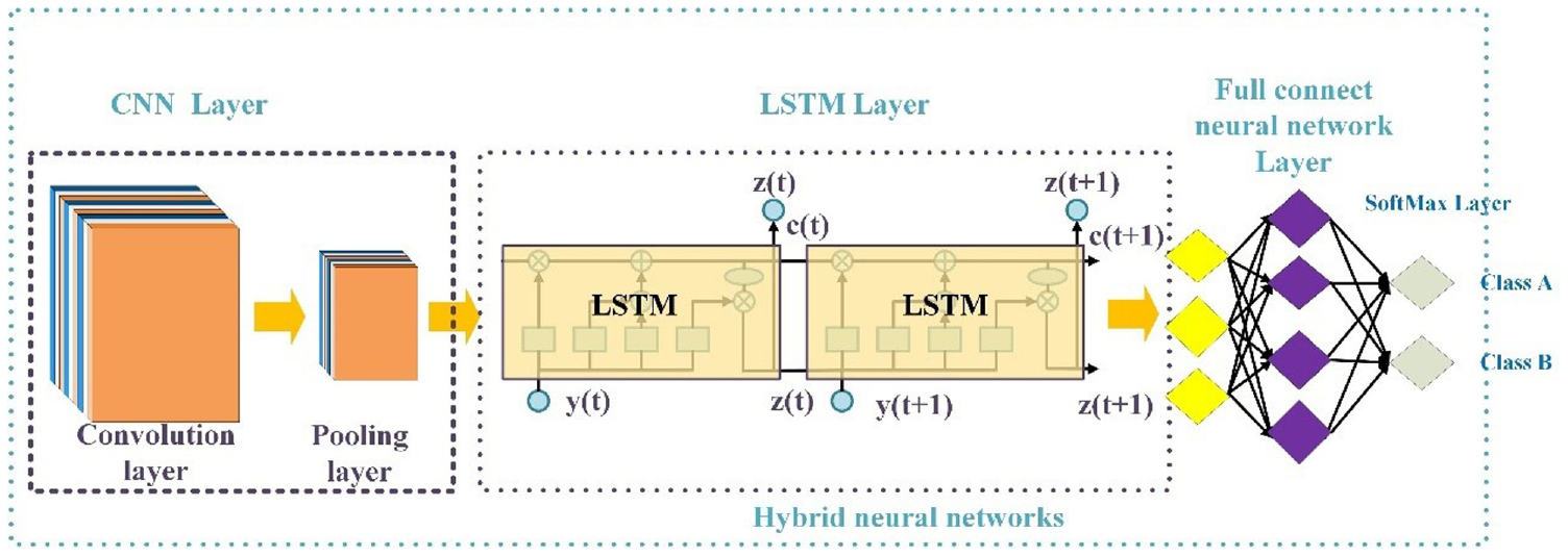
Proposed hybrid neural network for signal classification.

The Adam gradient descent algorithm is applied for model training;⁴¹ this algorithm is often adopted for weight optimization in deep neural networks. A rectified linear unit (ReLU) activation function was used for the FC layers.

Results

Experimental design

A photograph and schematic of the ball screw feed drive system used in this study are presented in Figures 7(a) and 7(b), respectively. This ball screw feed drive system was a single-axis machine tool designed in-house according to industry specifications. It was equipped with 2-kW, 3000-rpm servo motors (Taiwan Delta Electronics) and a 3-ψ, 220-V oil-cooling system. The temperature control accuracy was ±2°C, the precision of the mechanical structure was 5 µm, the repeatability was 2 µm, the maximum positioning speed of the motor was 48 m/min, and the acceleration produced by the motor at 3000 rpm was 1g. In this study, dataset was collected from the motor driver at the frequency of 8 kHz selected by acquisitioned software (Delta Electronics ASDA series).³⁸

Figure 7.

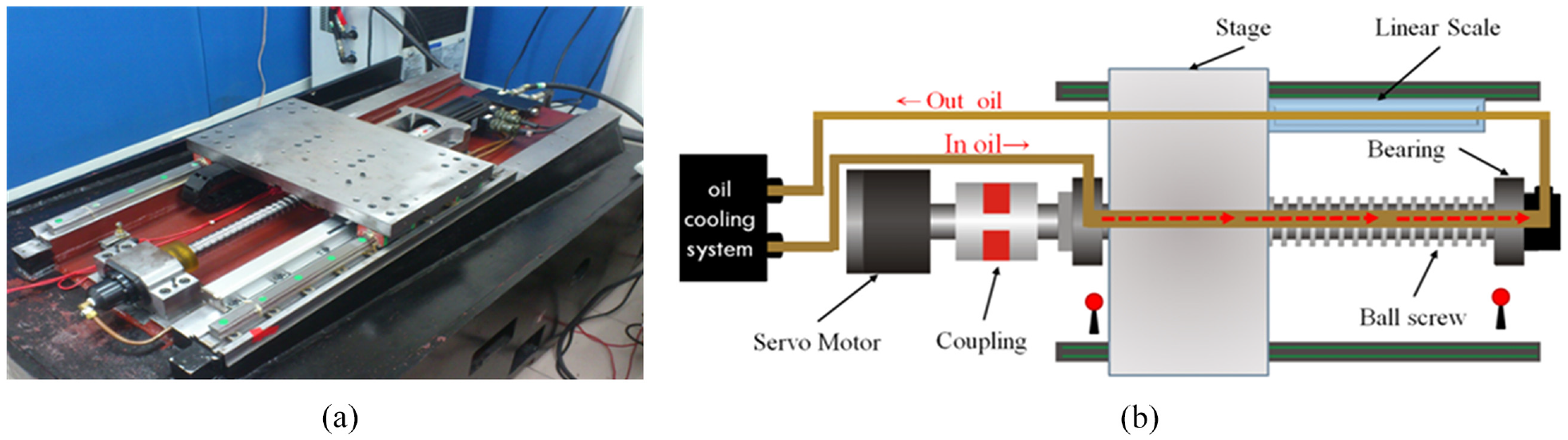
(a) Photograph and (b) schematic of a single-axis hollow ball screw platform that was designed in-house with a servo motor and linear scale positioning sensor.³⁸

For actual industrial operations, the pretension percentage of the standard precision motion ball screw is 4%, and the preloads on the hollow ball screw and the oil-cooling system are used to compensate for the heat effect to improve the positioning variation. A percentage preload of 2% results in the loss of preload force, which causes increases in the mechanical gap, increases in ball vibration, reductions in stiffness, and positioning errors. In this study, the experimental conditions of the hollow ball screw were as follows. For each test, a single type and a single condition were the independent variables, and the remaining conditions were control variables. At 15, 30, and 60 min after initiating the machine’s operation, the built-in signal was collected for 2 min at 15-, 30-, and 60-minute points during operation at a sampling frequency of 8 kHz. During the first stage of this experiment, conventional machine learning was adopted, and the most characteristic sensor signals were identified for classification. Figure 8 presents plots of the built-in signal data (e.g. servo motor current and rpm signal); this figure also includes the linear scale positioning signal from the reciprocating motion of the hollow ball screw.

Figure 8.

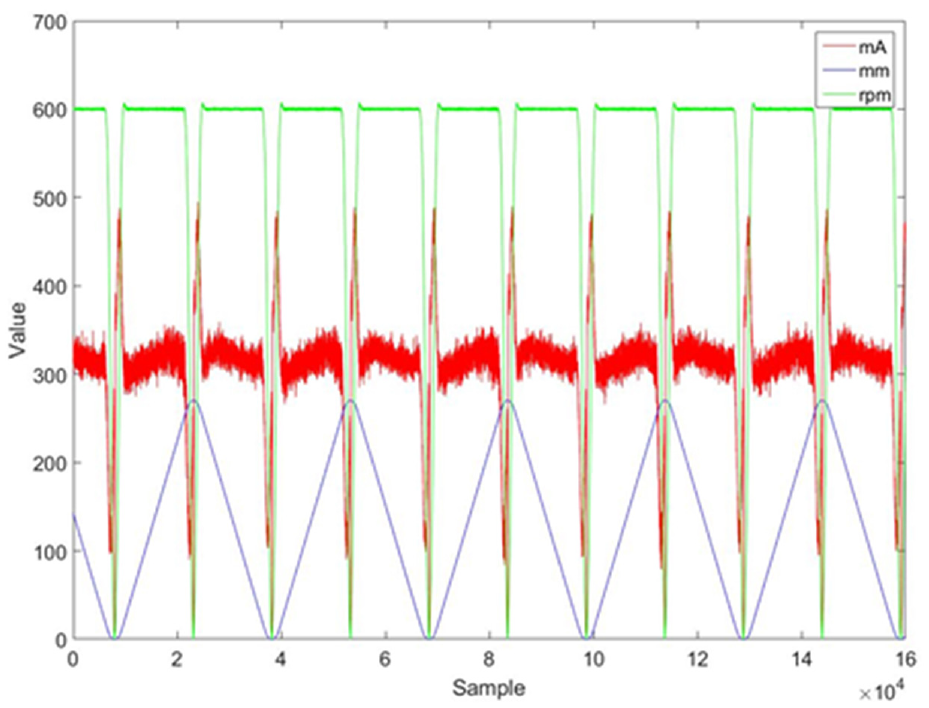
Current, position, and rpm of a fixed repeated path.³⁸

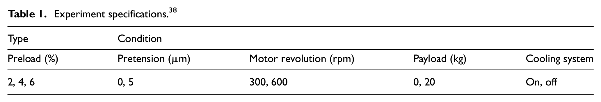
The original element engineering data were obtained from the experiment detailed in the following section. The experimental conditions and uniaxial reaction of the hollow ball screw are detailed in Table 1. Raw data were used as the input for feature engineering, which output the most distinctive signal. In Huang and Hsieh,³⁸ total 144 preload diagnosis experiments were conducted, for an example, 2 % ball screw preload nut with 4% ball screw preload nut. And three times of 72 experiments for every single preload ball screw nut, for an example of 6%, were performed for each of pretension diagnosis, payload diagnosis, and cooling system diagnosis. These experiments were performed using a data set for which conventional machine learning approaches have failed to yield good classification results to compare conventional machine learning and deep learning. A flow chart of the comparison is presented in Figure 9.

Table 1.

Experiment specifications.³⁸

Type	Condition
Preload (%)	Pretension (µm)	Motor revolution (rpm)	Payload (kg)	Cooling system
2, 4, 6	0, 5	300, 600	0, 20	On, off

Figure 9.

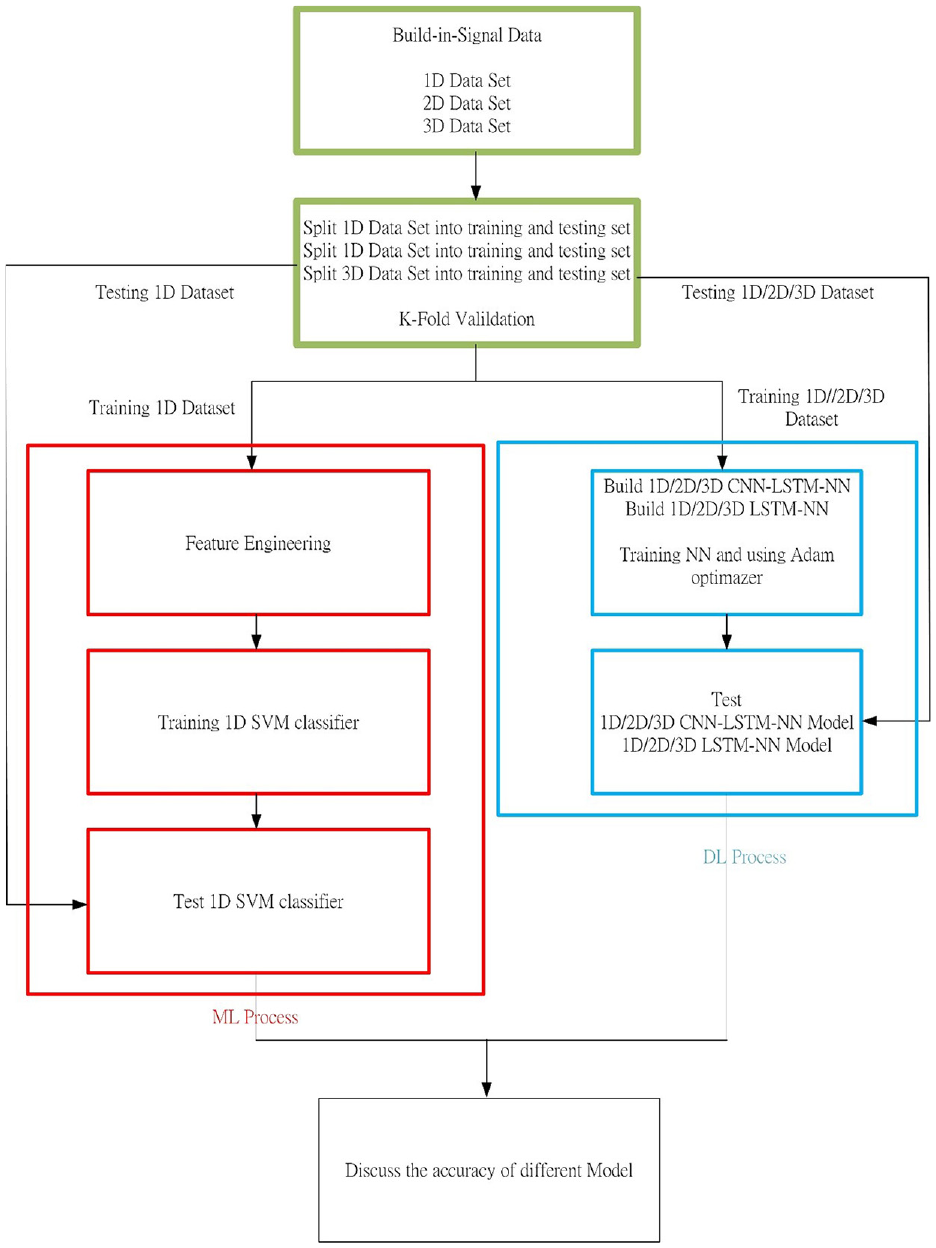
Flow chart for comparing the prediction accuracies of conventional machine learning and deep learning architectures.

A three-dimensional (3D) data set was used to represent the hallow ball screw; these dimensions were the motor’s current, motor’s rpm, and optical scale. These data were collected experimentally. Next, we divided the data equally into training and test sets by using five-fold verification. For the hybrid CNN–LSTM model (deep learning), we used 1D, 2D, and 3D data sets to train and test the network. For example, if we used only current, then the 1D data set was adopted. If both current and rpm were used, then the 2D data set was used. In a previous machine learning study,³⁸ feature engineering was performed first, with Fisher’s score as an indicator. For various preload classifications, current had the highest result for Fisher’s score (Figure 10). Among the three signals, the Fisher’s score, dispersion, and aggregation results were always highest for current, indicating that this is the most useful built-in signal. Fisher’s score was relatively low for the optical linear scale position and rpm signals, and partial overlapping was observed; thus, 1D data were used to train the SVM model in the conventional machine learning experiment. The optimization of SVM parameters is detailed in Huang and Hsieh.³⁸

Figure 10.

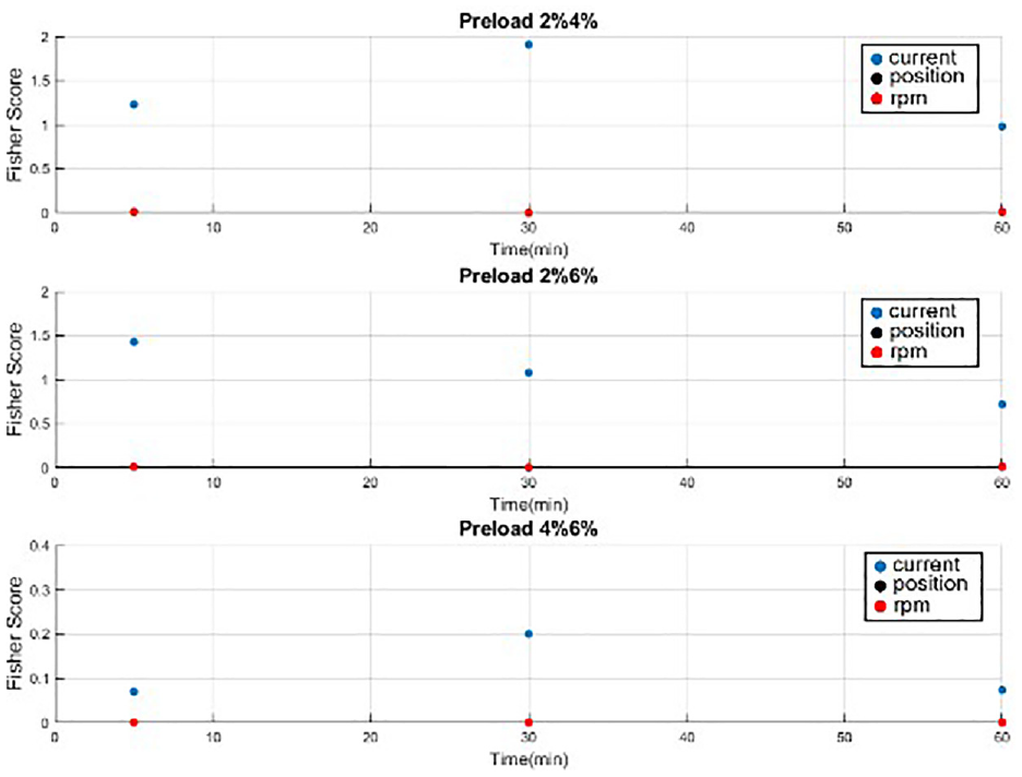
Comparative plots of Fisher’s score for current, linear scale, and rpm with a pretension of 0 µm and an oil-cooling system operated at 600 rpm.³⁸

Neural network parameters and hyperparameter experiments

The parameters and hyperparameters of a neural network must be adjusted to optimize the model performance. The notation for data set parameters is illustrated in Figure 11. In the experiments, the parameters 2%, C, 0 µm, 0 kg, 300 rpm, and 5 min and 2%, C, 5 µm, 0 kg, 300 rpm, and 5 min were tested for two-class classification, as displayed in Figure 12. In this parameter notation, 2% refers to a preload of 2%, C represents oil cooling, NC represents no oil cooling, 0 µm indicates a pretension of 0 µm, 0 kg refers to a payload of 0 kg, and 5 min is the motor load time; other parameters are detailed in Table 1.

Figure 11.

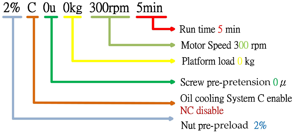
Notation for data set parameters.

Figure 12.

(a) Current, (b) position, and (c) rpm for the conditions 2%, C, 0 µm, 0 kg, 300 rpm, and 5 min (blue) and 2%, C, 5 µm, 0 kg, 300 rpm, and 5 min (orange).

The 3D data set included current, position, and rpm, with a total of 160,000 entries. We used 80,000 records as the training set, and the remaining 80,000 records were divided into five equal parts for verification.

LSTM network parameters and hyperparameter experiments

The neural network architecture shown in Figure 13 comprised an LSTM layer, a dropout layer, an FC layer, and finally a softmax layer for two output classes. The ReLU activation function was used in the FC layer, and the model was optimized using the Adam algorithm.

Figure 13.

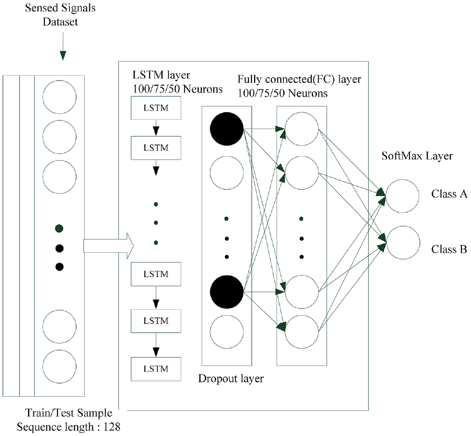
LSTM network for parameter experimentation.

LSTM network parameter experiment

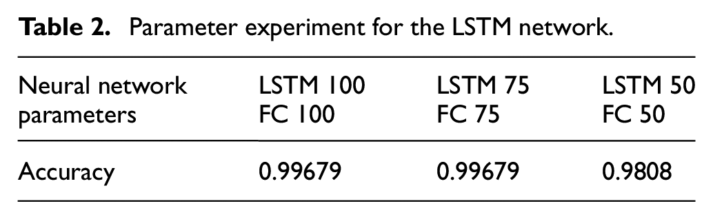
In this experiment, various parameters were used for the LSTM and FC layers to maximize the model accuracy and minimize the total number of neurons. The following hyperparameters were selected: 100 epochs, a batch size of 16, and a learning rate (lr) of 0.0001. The highest accuracy (0.99) was obtained by the model with 100 LSTM neurons and 100 FC neurons and by the model with 75 LSTM neurons and 75 FC neurons; the model with 50 LSTM neurons and 50 FC neurons obtained an accuracy of 0.98. Therefore, 75 LSTM neurons and 75 FC neurons maximized the accuracy and minimized the total number of neurons (Table 2).

Table 2.

Parameter experiment for the LSTM network.

Neural network parameters	LSTM 100	LSTM 75	LSTM 50
Neural network parameters	FC 100	FC 75	FC 50
Accuracy	0.99679	0.99679	0.9808

LSTM network hyperparameter experiment

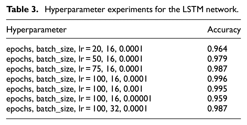
Next, we performed experiments to determine the most suitable hyperparameters for the architecture with 75 LSTM neurons and 75 FC neurons. The goal was to minimize the number of epochs and batch size and maximize the accuracy. First, the batch size was set as 16 and the lr was set at 0.0001, and we trained and tested the network with 20, 50, 75, and 100, epochs. The accuracies of these models were 0.964, 0.979, 0.987, and 0.996, respectively. Thus, 100 epochs yielded the highest accuracy. The number of epochs and batch size were then set at 100 and 16, respectively, and we trained and tested the network with lr values of 0.001 and 0.00001. These models yielded accuracies of 0.995 and 0.959, respectively. Because these results were both less than 0.996, we set the number of epochs as 100 and lr as 0.0001, and we trained and tested the network with batch sizes of 16 and 32. The accuracies of these models were 0.996 and 0.987, respectively (Table 3). Therefore, the following hyperparameters were selected: 100 epochs, a batch size of 16, and an lr of 0.0001. Figure 14 indicates that the training loss converged after 100 epochs with a value of 0.0178.

Table 3.

Hyperparameter experiments for the LSTM network.

Hyperparameter	Accuracy
epochs, batch_size, lr = 20, 16, 0.0001	0.964
epochs, batch_size, lr = 50, 16, 0.0001	0.979
epochs, batch_size, lr = 75, 16, 0.0001	0.987
epochs, batch_size, lr = 100, 16, 0.0001	0.996
epochs, batch_size, lr = 100, 16, 0.001	0.995
epochs, batch_size, lr = 100, 16, 0.00001	0.959
epochs, batch_size, lr = 100, 32, 0.0001	0.987

Figure 14.

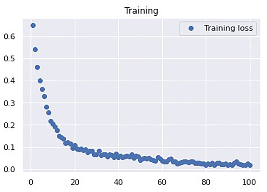
LSTM loss function curve.

LSTM accuracy with 1D, 2D, and 3D data sets

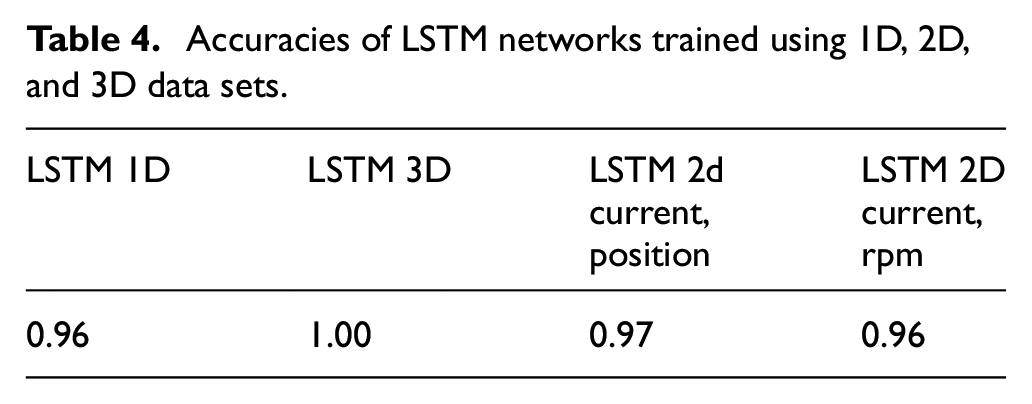
With the aforementioned optimal parameters and hyperparameters, the accuracies of the LSTM models trained using the 1D (current), 3D (current, position, and rpm), 2D (current and position), and 2D (current and rpm) data sets were 0.96, 1, 0.97, and 0.96, respectively. Therefore, subsequent experiments were performed using the 1D and 3D data sets for the LSTM model (Table 4).

Table 4.

Accuracies of LSTM networks trained using 1D, 2D, and 3D data sets.

LSTM 1D	LSTM 3D	LSTM 2d current, position	LSTM 2D current, rpm
0.96	1.00	0.97	0.96

Type-1 CNN–LSTM network parameters and hyperparameter experiments

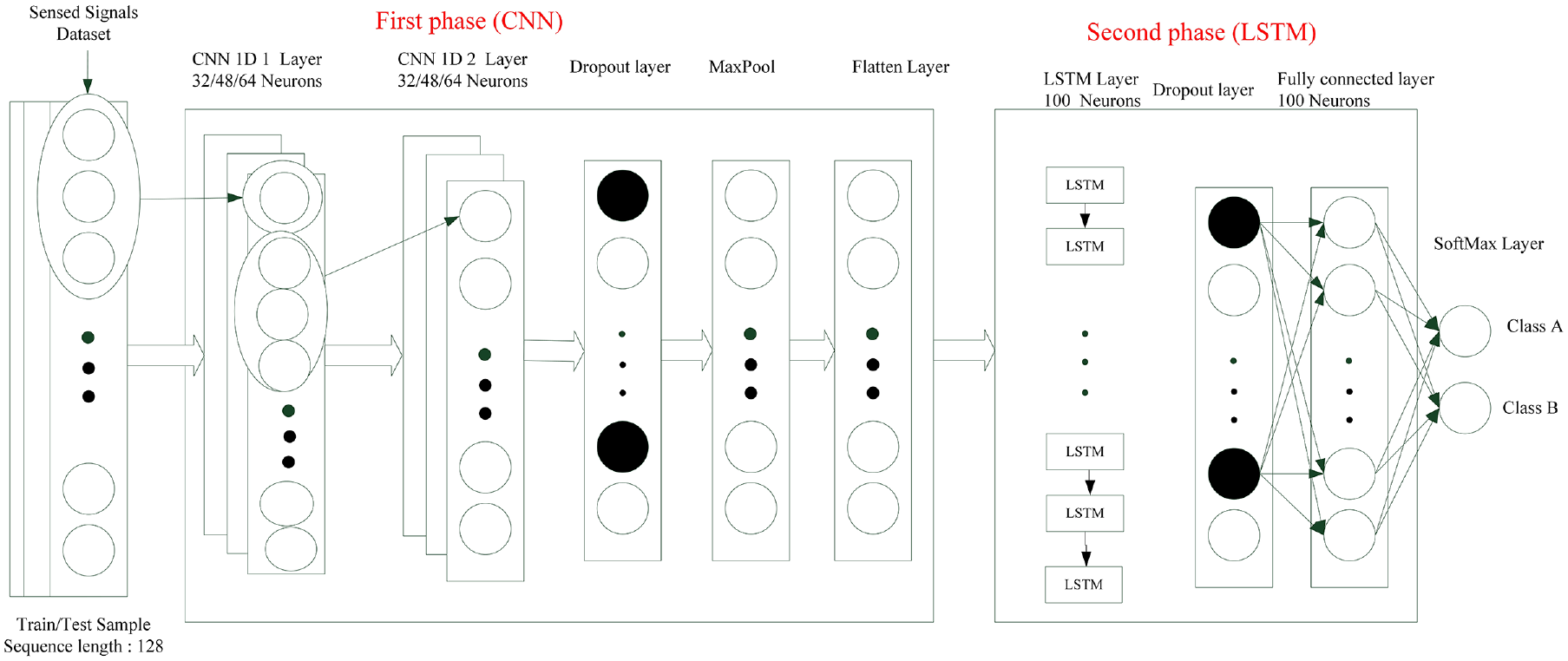
The neural network architecture shown in Figure 15 comprised a CNN layer, a dropout layer, a maximum pooling layer, a flatten layer, an LSTM layer, another dropout layer, an FC layer, and finally a softmax for two output classes. The activation function for the FC layers was ReLU, and the model was optimized using the Adam algorithm.

Figure 15.

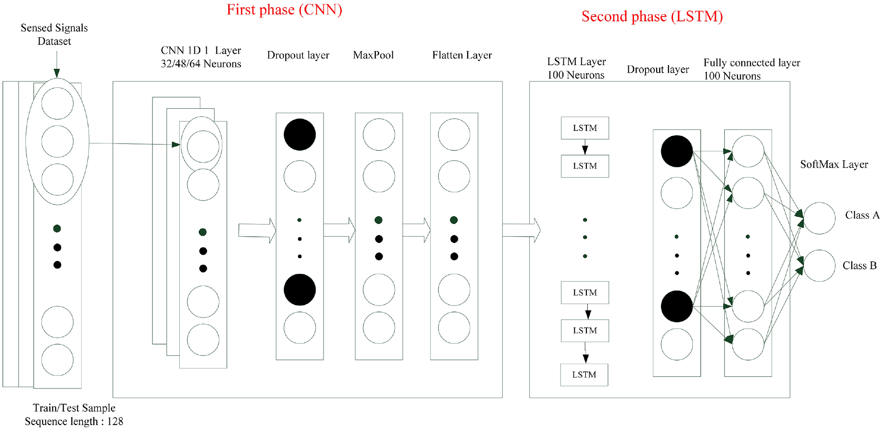
Type-1 CNN–LSTM network for parameter experimentation.

Type-1 CNN–LSTM network parameter experiment

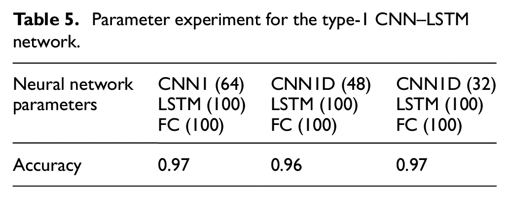
Various parameters were used for the 1D CNN, LSTM, and FC layers, to maximize the model accuracy and minimize the total number of neurons. The following hyperparameters were selected: 100 epochs, a batch size of 64, and an lr of 0.0001. The accuracy of the model with 64 1D CNN neurons, 100 LSTM neurons, and 100 FC neurons was 0.97; that of the model with 48 1D CNN neurons, 100 LSTM neurons, and 100 FC neurons was 0.96, which was the lowest accuracy in the experiment; that of the model with 32 CNN1 neurons, 100 LSTM neurons, and 100 FC neurons was 0.97, which was the highest accuracy. This model also minimized the total number of neurons (Table 5).

Table 5.

Parameter experiment for the type-1 CNN–LSTM network.

Neural network parameters	CNN1 (64)	CNN1D (48)	CNN1D (32)
	LSTM (100)	LSTM (100)	LSTM (100)
	FC (100)	FC (100)	FC (100)
Accuracy	0.97	0.96	0.97

Type-1 CNN–LSTM network hyperparameter experiment

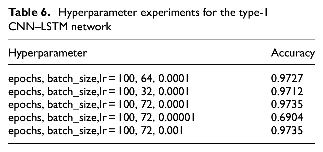
Next, we performed experiments to determine the most suitable hyperparameters for the architecture with 64 1D CNN neurons, 100 LSTM neurons, and 100 FC neurons. The goal was to minimize the number of epochs and batch size and maximize the accuracy. First, we set the number of epochs to 100 and the lr to 0.0001, and we trained and tested the network with batch sizes of 64, 32, and 72. The accuracies of these models were 0.9727, 0.9712, and 0.9735, respectively. Therefore, the batch size of 72 yielded the highest accuracy. We then set the batch size to 72 and the number of epochs to 100, and we trained and tested the network with lr values of 0.001 and 0.00001. The accuracies of these models were 0.6904 and 0.9735, respectively (Table 6). Therefore, we adopted an lr of 0.0001 and 100 epochs for the Type-1 CNN–LSTM architecture. Because this model was more complex than the previous LSTM model, the number of epochs required for convergence was higher. As shown in Figure 16, the loss value was 0.110 after 100 epochs for the Type-1 CNN–LSTM.

Table 6.

Hyperparameter experiments for the type-1 CNN–LSTM network

Hyperparameter	Accuracy
epochs, batch_size,lr = 100, 64, 0.0001	0.9727
epochs, batch_size,lr = 100, 32, 0.0001	0.9712
epochs, batch_size,lr = 100, 72, 0.0001	0.9735
epochs, batch_size,lr = 100, 72, 0.00001	0.6904
epochs, batch_size,lr = 100, 72, 0.001	0.9735

Figure 16.

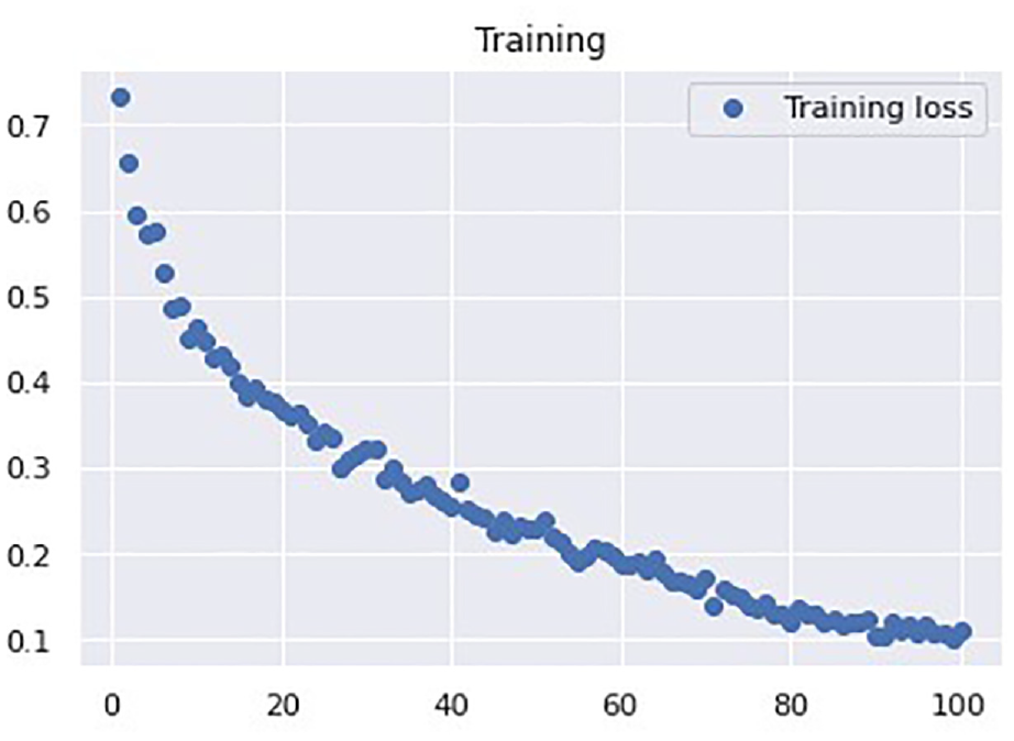
Type-1 CNN–LSTM loss function curve.

Type-1 CNN–LSTM accuracy with 1D, 2D, and 3D data sets

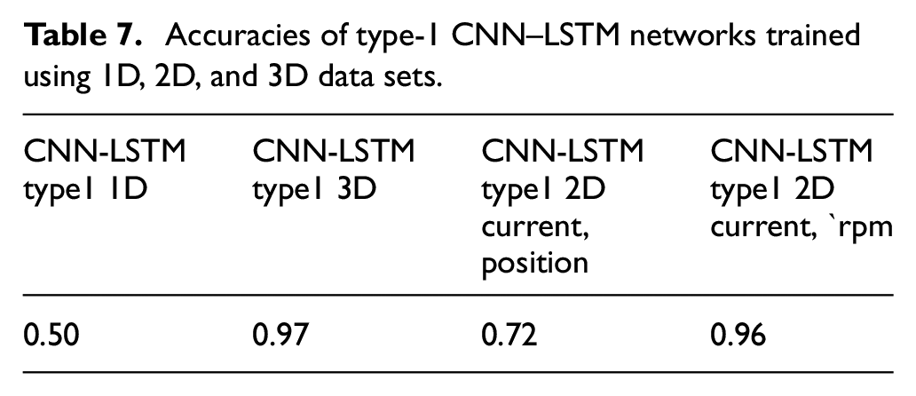
With the aforementioned optimal parameters and hyperparameters, the accuracies of the Type-1 CNN–LSTM models trained using 1D (current), 3D (current, position, and rpm), 2D (current and position), and 2D (current and rpm) data sets were 0.50, 0.97, 0.72, and 0.96, respectively. Although the position signal is presented separately in Figure 13 because of its mechanical characteristics, it was unhelpful for neural network training. Therefore, subsequent experiments were performed using the 1D and 3D data sets for the Type-1 CNN–LSTM model (Table 7).

Table 7.

Accuracies of type-1 CNN–LSTM networks trained using 1D, 2D, and 3D data sets.

CNN-LSTM type1 1D	CNN-LSTM type1 3D	CNN-LSTM type1 2D current, position	CNN-LSTM type1 2D current, \lsquorpm
0.50	0.97	0.72	0.96

Type-2 CNN–LSTM network parameters and hyperparameter experiments

The neural network architecture displayed in Figure 17 comprised two 1D CNN layers, a dropout layer, a maximum pooling layer, a flatten layer, an LSTM layer, a dropout layer, an FC layer, and finally a softmax layer for two output classes. The activation function for the FC layer was ReLU, and the model was optimized using the Adam algorithm.

Figure 17.

Type-2 CNN–LSTM network for parameter experimentation.

Type-2 CNN–LSTM network parameter experiment

In this experiment, various parameters were used for the 1D CNN, LSTM, and FC layers to maximize the model accuracy and minimize the total number of neurons. The following hyperparameters were selected: 100 epochs, a batch size of 64, and an lr of 0.0001.

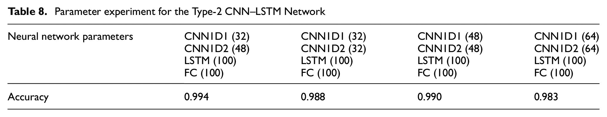
The accuracy of the model with 32 + 48 1D CNN neurons, 100 LSTM neurons, and 100 FC neurons was 0.994, and that of the model with 32 + 32 1D CNN neurons, 100 LSTM neurons, and 100 FC neurons was 0.988. Moreover, the accuracy of the model with 48 + 48 1D CNN neurons, 100 LSTM neurons, and 100 FC neurons was 0.990, and that of the model with 64 + 64 1D CNN neurons, 100 LSTM neurons, and 100 FC neurons was 0.983. Thus, the model with 32 + 48 1D CNN neurons, 100 LSTM neurons, and 100 FC neurons achieved the highest accuracy (Table 8).

Table 8.

Parameter experiment for the Type-2 CNN–LSTM Network

Neural network parameters	CNN1D1 (32)	CNN1D1 (32)	CNN1D1 (48)	CNN1D1 (64)
	CNN1D2 (48)	CNN1D2 (32)	CNN1D2 (48)	CNN1D2 (64)
	LSTM (100)	LSTM (100)	LSTM (100)	LSTM (100)
	FC (100)	FC (100)	FC (100)	FC (100)
Accuracy	0.994	0.988	0.990	0.983

Type-2 CNN–LSTM

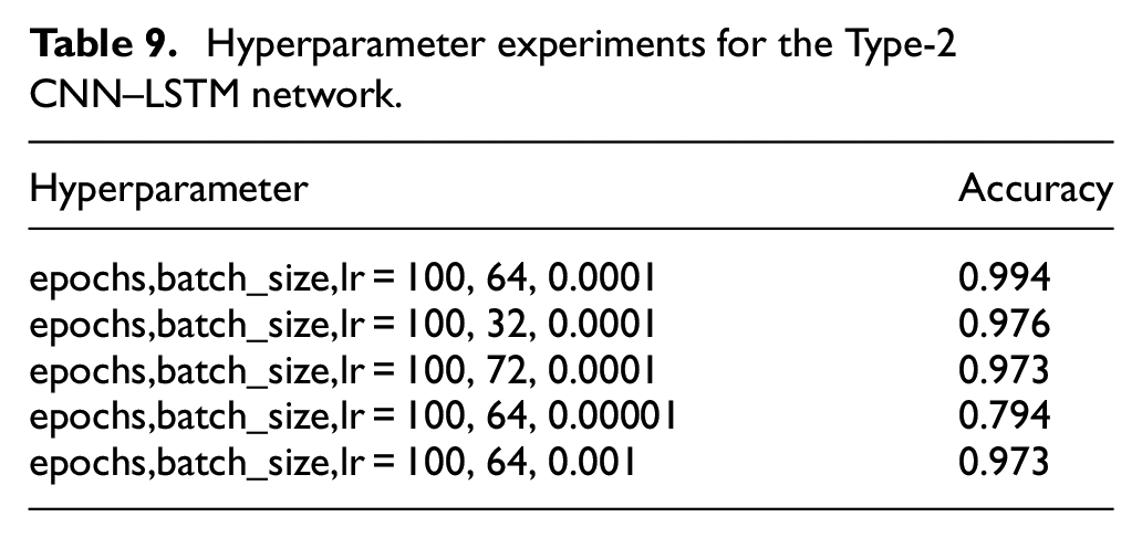
Next, we performed experiments to determine the most suitable hyperparameters using 32 + 48 1D CNN neurons, 100 LSTM neurons, and 100 FC neurons. The goal was to minimize the number of epochs and batch size and maximize the accuracy. First, we set the number of epochs to 100 and the lr to 0.0001, and we trained and tested the network with batch sizes of 64, 32, and 72. The accuracies of these models were 0.9944, 0.9768, 0.9732, respectively. Therefore, the batch size of 64 yielded the maximum accuracy. Next, we set the batch size to 64 and the number of epochs to 100, and we trained and tested the network with lr values of 0.00001 and 0.001. The accuracies of these models were 0.794 and 0.973, respectively; thus, both were less than 0.994 (Table 9). The structure of the Type-2 CNN–LSTM is more complex than that of the Type-1 CNN–LSTM and LSTM models. Therefore, the number of epochs required for convergence for the Type-2 CNN–LSTM model was not lower than that for the Type-1 CNN–LSTM and LSTM models. With 100 epochs, the loss value of the Type-2 CNN–LSTM model appeared to converge (Figure 18).

Table 9.

Hyperparameter experiments for the Type-2 CNN–LSTM network.

Hyperparameter	Accuracy
epochs,batch_size,lr = 100, 64, 0.0001	0.994
epochs,batch_size,lr = 100, 32, 0.0001	0.976
epochs,batch_size,lr = 100, 72, 0.0001	0.973
epochs,batch_size,lr = 100, 64, 0.00001	0.794
epochs,batch_size,lr = 100, 64, 0.001	0.973

Figure 18.

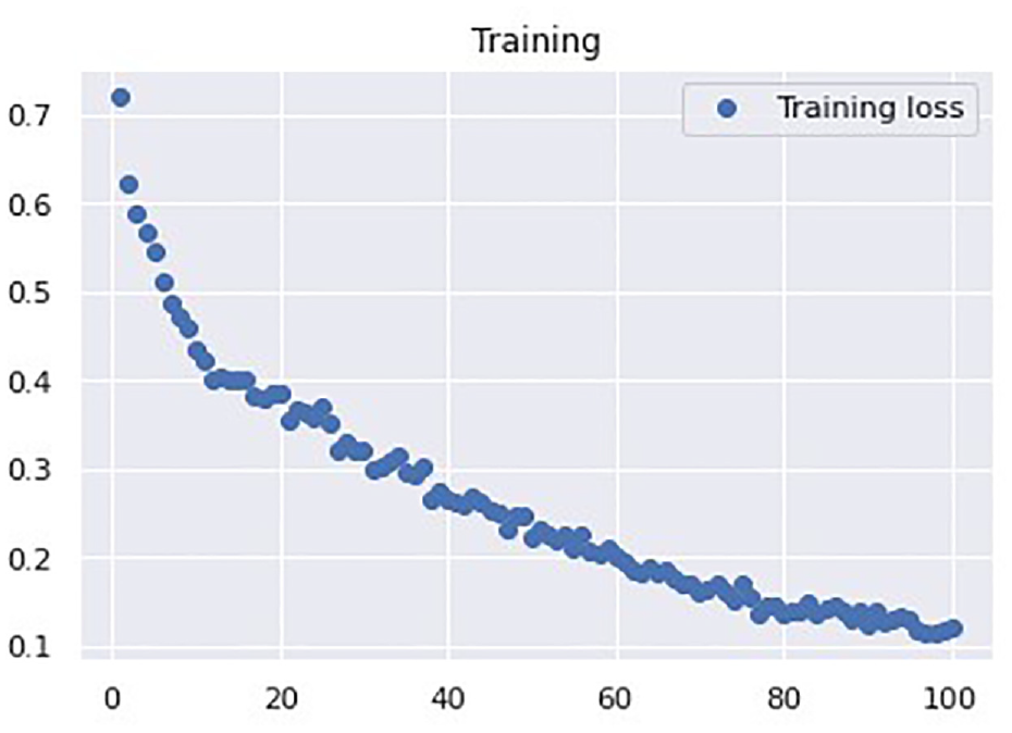
Type-2 CNN–LSTM loss function curve.

Type-2 CNN–LSTM accuracy with 1D, 2D, and 3D data sets

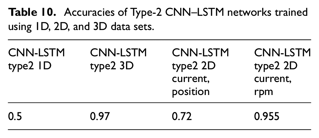
With the aforementioned optimal parameters and hyperparameters, the accuracies of the Type-2 CNN–LSTM models trained using the 1D (current), 3D (current, position, and rpm), 2D (current and position), and 2D (current and rpm) data sets were 0.50, 0.97, 0.72, and 0.955, respectively. Although the optical scale signal is presented separately in Figure 13 because of its mechanical characteristics, it was unhelpful for neural network training. Therefore, subsequent experiments were performed using the 1D and 3D data sets for the Type-2 CNN–LSTM model (Table 10).

Table 10.

Accuracies of Type-2 CNN–LSTM networks trained using 1D, 2D, and 3D data sets.

CNN-LSTM type2 1D	CNN-LSTM type2 3D	CNN-LSTM type2 2D current, position	CNN-LSTM type2 2D current, rpm
0.5	0.97	0.72	0.955

Comparison of the LSTM, Type-1 CNN–LSTM, and Type-2 CNN–LSTM networks with different data sets

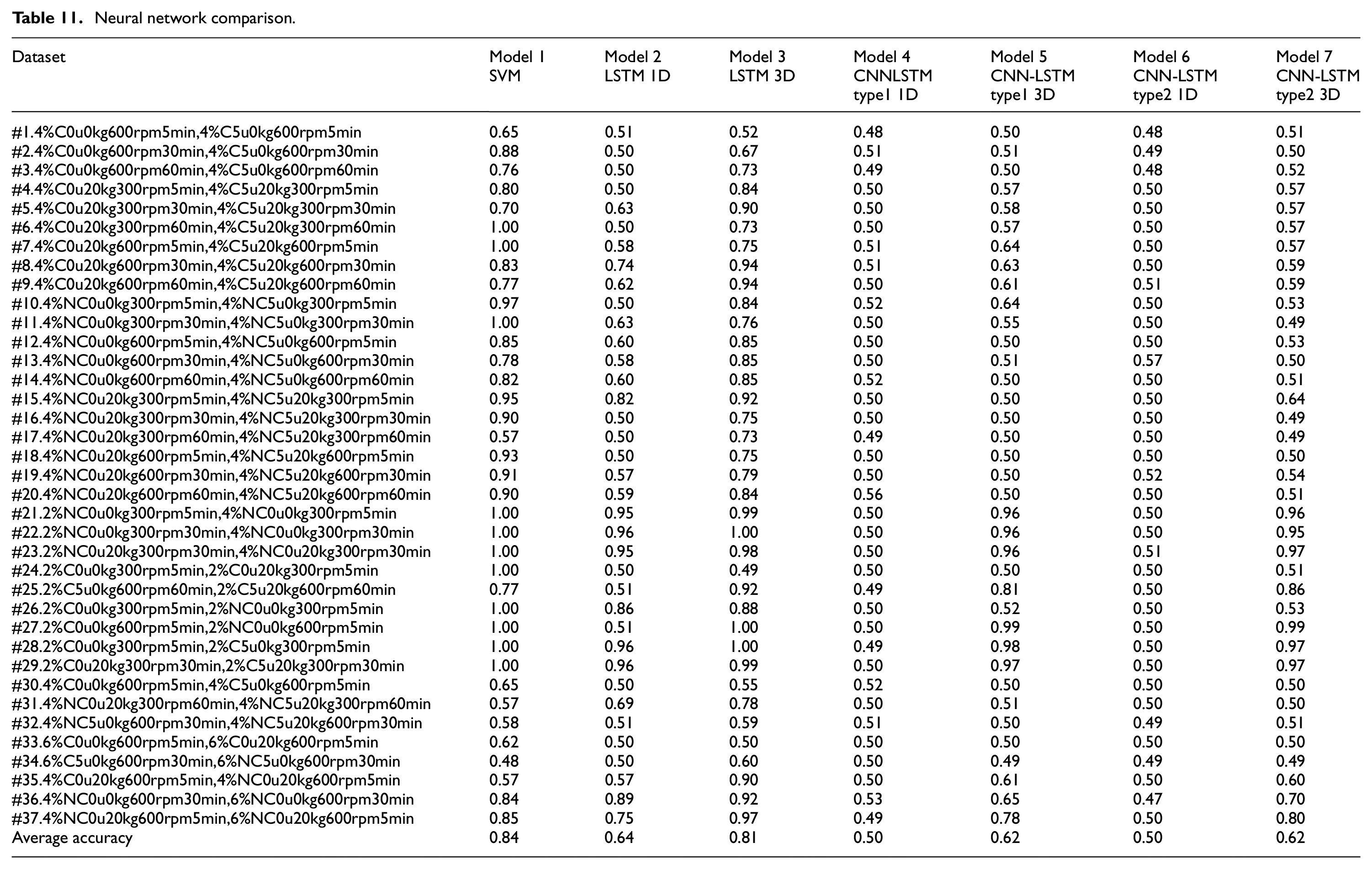
A number of total 144 experimental data sets were conducted in Huang and Hsieh.³⁸ There were total 360 models by the method of feature engineering and SVM classification. In following study, 37 data sets were selected for the comparison with proposed DNN neural networks. Table 11 lists the results of the experiments comparing the performance of the SVM³⁸ and deep learning models with 37 different data sets. These deep learning models used the parameters obtained as described in Sections 3.3–3.5. The seven models with the highest accuracies are detailed as follows.

Model 1: SVM with six time-domain features and 88 frequency-domain features extracted through feature engineering. For the frequency-domain features, the current training number yielded a higher Fisher’s score. The most distinctive data determined through the standard Fisher’s survey were used to select the most distinctive feature set to train the SVM. The SVM algorithm optimizes the parameters σ and C within the range of 2⁻⁵–2⁵.³⁸

Model 2: 1D LSTM with 75 LSTM neurons and 75 FC neurons. The model was trained for 100 epochs with a batch size of 16 and an lr of 0.0001. The activation function for the FC layer was ReLU, the model was optimized using the Adam algorithm, and the current signal was used for training and testing.

Model 3: 3D LSTM with 75 LSTM neurons and 75 FC neurons. The model was trained for 100 epochs with a batch size of 16 and an lr of 0.0001. The activation function for the FC layer was ReLU, the model was optimized using the Adam algorithm, and the current, position, and rpm signals were used for training and testing.

Model 4: 1D Type-1 CNN–LSTM with 64 CNN neurons, 100 LSTM neurons, and 100 FC neurons. The model was trained for 100 epochs with a batch size of 72 and an lr of 0.0001. The activation function for the FC layer was ReLU, the model was optimized using the Adam algorithm, and the current signal was used for training and testing.

Model 5: 3D Type-1 CNN–LSTM with 64 CNN neurons, 100 LSTM neurons, and 100 FC neurons. The model was trained for 100 epochs with a batch size of 72 and an lr of 0.0001. The activation function for the FC layer was ReLU, the model was optimized using the Adam algorithm, and the current signal was used for training and testing.

Model 6: 1D Type-2 CNN–LSTM with 32 + 48 CNN neurons, 100 LSTM neurons, and 100 FC neurons. The model was trained for 100 epochs with a batch size of 64 and an lr of 0.0001. The activation function for the FC layer was ReLU, the model was optimized using the Adam algorithm, and the current, position, and rpm signals were used for training and testing.

Model 7: 3D Type-2 CNN–LSTM with 32 + 48 CNN neurons, 100 LSTM neurons, and 100 FC neurons. The model was trained for 100 epochs with a batch size of 64 and an lr of 0.0001. The activation function for the FC layer was ReLU, the model was optimized using the Adam algorithm, and the current, position, and rpm signals were used for training and testing.

Table 11.

Neural network comparison.

Dataset	Model 1	Model 2	Model 3	Model 4	Model 5	Model 6	Model 7
Dataset	SVM	LSTM 1D	LSTM 3D	CNNLSTM type1 1D	CNN-LSTM type1 3D	CNN-LSTM type2 1D	CNN-LSTM type2 3D
#1.4%C0u0kg600rpm5min,4%C5u0kg600rpm5min	0.65	0.51	0.52	0.48	0.50	0.48	0.51
#2.4%C0u0kg600rpm30min,4%C5u0kg600rpm30min	0.88	0.50	0.67	0.51	0.51	0.49	0.50
#3.4%C0u0kg600rpm60min,4%C5u0kg600rpm60min	0.76	0.50	0.73	0.49	0.50	0.48	0.52
#4.4%C0u20kg300rpm5min,4%C5u20kg300rpm5min	0.80	0.50	0.84	0.50	0.57	0.50	0.57
#5.4%C0u20kg300rpm30min,4%C5u20kg300rpm30min	0.70	0.63	0.90	0.50	0.58	0.50	0.57
#6.4%C0u20kg300rpm60min,4%C5u20kg300rpm60min	1.00	0.50	0.73	0.50	0.57	0.50	0.57
#7.4%C0u20kg600rpm5min,4%C5u20kg600rpm5min	1.00	0.58	0.75	0.51	0.64	0.50	0.57
#8.4%C0u20kg600rpm30min,4%C5u20kg600rpm30min	0.83	0.74	0.94	0.51	0.63	0.50	0.59
#9.4%C0u20kg600rpm60min,4%C5u20kg600rpm60min	0.77	0.62	0.94	0.50	0.61	0.51	0.59
#10.4%NC0u0kg300rpm5min,4%NC5u0kg300rpm5min	0.97	0.50	0.84	0.52	0.64	0.50	0.53
#11.4%NC0u0kg300rpm30min,4%NC5u0kg300rpm30min	1.00	0.63	0.76	0.50	0.55	0.50	0.49
#12.4%NC0u0kg600rpm5min,4%NC5u0kg600rpm5min	0.85	0.60	0.85	0.50	0.50	0.50	0.53
#13.4%NC0u0kg600rpm30min,4%NC5u0kg600rpm30min	0.78	0.58	0.85	0.50	0.51	0.57	0.50
#14.4%NC0u0kg600rpm60min,4%NC5u0kg600rpm60min	0.82	0.60	0.85	0.52	0.50	0.50	0.51
#15.4%NC0u20kg300rpm5min,4%NC5u20kg300rpm5min	0.95	0.82	0.92	0.50	0.50	0.50	0.64
#16.4%NC0u20kg300rpm30min,4%NC5u20kg300rpm30min	0.90	0.50	0.75	0.50	0.50	0.50	0.49
#17.4%NC0u20kg300rpm60min,4%NC5u20kg300rpm60min	0.57	0.50	0.73	0.49	0.50	0.50	0.49
#18.4%NC0u20kg600rpm5min,4%NC5u20kg600rpm5min	0.93	0.50	0.75	0.50	0.50	0.50	0.50
#19.4%NC0u20kg600rpm30min,4%NC5u20kg600rpm30min	0.91	0.57	0.79	0.50	0.50	0.52	0.54
#20.4%NC0u20kg600rpm60min,4%NC5u20kg600rpm60min	0.90	0.59	0.84	0.56	0.50	0.50	0.51
#21.2%NC0u0kg300rpm5min,4%NC0u0kg300rpm5min	1.00	0.95	0.99	0.50	0.96	0.50	0.96
#22.2%NC0u0kg300rpm30min,4%NC0u0kg300rpm30min	1.00	0.96	1.00	0.50	0.96	0.50	0.95
#23.2%NC0u20kg300rpm30min,4%NC0u20kg300rpm30min	1.00	0.95	0.98	0.50	0.96	0.51	0.97
#24.2%C0u0kg300rpm5min,2%C0u20kg300rpm5min	1.00	0.50	0.49	0.50	0.50	0.50	0.51
#25.2%C5u0kg600rpm60min,2%C5u20kg600rpm60min	0.77	0.51	0.92	0.49	0.81	0.50	0.86
#26.2%C0u0kg300rpm5min,2%NC0u0kg300rpm5min	1.00	0.86	0.88	0.50	0.52	0.50	0.53
#27.2%C0u0kg600rpm5min,2%NC0u0kg600rpm5min	1.00	0.51	1.00	0.50	0.99	0.50	0.99
#28.2%C0u0kg300rpm5min,2%C5u0kg300rpm5min	1.00	0.96	1.00	0.49	0.98	0.50	0.97
#29.2%C0u20kg300rpm30min,2%C5u20kg300rpm30min	1.00	0.96	0.99	0.50	0.97	0.50	0.97
#30.4%C0u0kg600rpm5min,4%C5u0kg600rpm5min	0.65	0.50	0.55	0.52	0.50	0.50	0.50
#31.4%NC0u20kg300rpm60min,4%NC5u20kg300rpm60min	0.57	0.69	0.78	0.50	0.51	0.50	0.50
#32.4%NC5u0kg600rpm30min,4%NC5u20kg600rpm30min	0.58	0.51	0.59	0.51	0.50	0.49	0.51
#33.6%C0u0kg600rpm5min,6%C0u20kg600rpm5min	0.62	0.50	0.50	0.50	0.50	0.50	0.50
#34.6%C5u0kg600rpm30min,6%NC5u0kg600rpm30min	0.48	0.50	0.60	0.50	0.49	0.49	0.49
#35.4%C0u20kg600rpm5min,4%NC0u20kg600rpm5min	0.57	0.57	0.90	0.50	0.61	0.50	0.60
#36.4%NC0u0kg600rpm30min,6%NC0u0kg600rpm30min	0.84	0.89	0.92	0.53	0.65	0.47	0.70
#37.4%NC0u20kg600rpm5min,6%NC0u20kg600rpm5min	0.85	0.75	0.97	0.49	0.78	0.50	0.80
Average accuracy	0.84	0.64	0.81	0.50	0.62	0.50	0.62

Neural network comparison

A total of 37 data sets were applied to compare the prediction accuracies of the SVM and deep learning models. For the deep learning models, the experimental parameters obtained as described in Sections 3.3–3.5 were adopted.

As shown in Table 11 and Figure 19, the highest accuracy was obtained for the SVM, followed by the 3D LSTM. The accuracy of the 3D LSTM was higher than that of the 1D LSTM; this result is attributable to the fact that the characteristics and diversity of 1D data sets cannot be effectively utilized in deep learning. The accuracies of the 1D LSTM and 3D LSTM were higher than those of the 1D Type-1 CNN–LSTM, 3D Type-1 CNN–LSTM, 1D Type-2 CNN–LSTM, and 3D Type-2 CNN–LSTM. This indicates that either the CNN–LSTM architecture did not effectively extract features from this data set or the complexity of the data set was insufficient for obtaining accurate results using this architecture. The decrease in prediction accuracy after the CNN was introduced to the hybrid CNN-LSTM model (models 4–7) may be attributable to the subsampling and filtering mechanism of the CNN. The digital data manipulation but not image manipulation of the CNN could blur the trend of the mechanical conditions of the ball screw. The deployment of feature engineering before model training in the SVM model may have resulted in its higher prediction accuracy relative to the LSTM model. Some outliers were removed during FE on the basis of statistical calculations. Additionally, the SVM parameters were optimized before prediction. By contrast, no outlying data were removed before the deep learning models were trained. The average accuracy of the 3D Type-1 CNN–LSTM and 3D Type-2 CNN–LSTM (0.62) was higher than that of the 1D Type-1 CNN–LSTM and 1D Type-2 CNN–LSTM (0.52). The complexity of the 3D data set was higher than that of the 1D data set, and the greater diversity of the training samples enhanced training in the deep learning models. A greater number of parameters can enable a neural network to be trained to achieve a higher accuracy. The average accuracy of the 3D Type-2 CNN–LSTM was the same as that of the 3D Type-1 CNN–LSTM, and the average accuracy of the 1D Type-2 CNN–LSTM was the same as that of the 1D Type-1 CNN–LSTM. Therefore, the additional CNN layer did not improve feature extraction.

Figure 19.

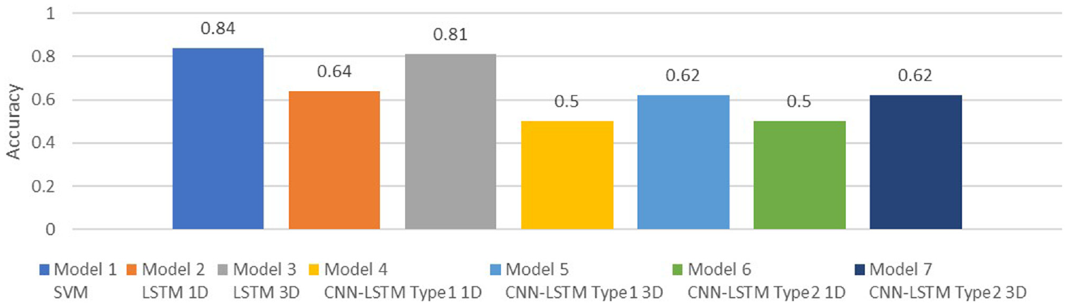
Neural network comparison.

Discussion

In this section we will discuss the results of 37 numerical simulations in Table 11. Features of every model will be compared with the others models based on the result of prediction accuracy in Section 4.1–Section 4.4. The characteristics of hollow ball screw with or without the preload, pretension, oil cooling system and payload are deliberated for the performance of predicted accuracy of the proposed models in Sections 4.5–Section 4.7.

Experiments 1–20: Applications for the standard 4% preload ball screw

A preload of 4% is standard for typical precision motion in industrial applications. In this study, the pretension and oil-cooling system on the hollow ball screw were used to compensate for thermal rigidity and thus improve the positioning accuracy. Changes in these conditions were regarded as features for classification. For experiments 1–3 and 7–9 (Model 3), the prediction accuracy increased with the training time. This indicates the advantage of using an LSTM model for sequential data. Experiments 1–20 revealed that the prediction accuracy of Model 3 was higher than that of Model 2, that of Model 5 was higher than that of Model 4, and that of Model 7 was higher than that of Model 6. Using the 3D data set rather than the 1D data set improved the prediction accuracy of the LSTM and hybrid CNN–LSTM deep learning models. In addition, according to the results of experiments 1–20, the prediction accuracies of Models 4–7 (approximately 0.5) were lower than those of the SVM and the 1D and 3D LSTM models.

Experiments 21–23 and 36–37: Comparisons for the 2% preload loss with standard 4% preload ball screw

A preload of 6% increased the contact force between the ball nut and the ball screw race relative to the standard preload of 4%. Moreover, a 2% preload would increase the mechanical backlash, increase the pitted ball trace, reduce the natural stiffness, and introduce oscillatory position errors. Experiments 21–23 yielded a high prediction accuracy. The SVM algorithm maps the input data into a higher-dimensional feature space based on the selection of a suitable kernel function. In Huang and Hsieh,³⁸ FE was implemented before the SVM’s supervised learning process was initiated; thus, an accuracy of almost 100% was achieved. However, in Models 2, 3, 6, and 7 (LSTM), the accuracy was also relatively high. In addition, the accuracy of the 3D LSTM model (Model 2) was higher than that of the 1D LSTM model (Model 3). Combining the LSTM model with a CNN (Models 4 and 6) did not improve the prediction accuracy, even though differences between the typed ball screws with preloads of 2% and 4% are relatively easy to classify. The results of experiments 36 and 37 suggest that the classification rate for the 2% preload condition was not higher than that for the 4% preload condition. This is because the 4% and 6% preloads of the ball screw should dominate its rigidity and firm motion behavior. Nevertheless, comparisons of Models 2 and 3, 4 and 5, and 6 and 7 revealed that the prediction accuracies of the 3D LSTM models were higher than those of the 1D LSTM models. Additional input data without FE retained good prediction accuracy for the LSTM deep learning approach.

Experiments 24–29: 2% preload loss ball screw under the circumstances of applying oil cooling system

The choice of pretension and oil-cooling system for the hollow ball screw were used to compensate for thermal rigidity and thus improve the positioning accuracy. The payload on the table generally had a limited effect of the diagnosis of the ball screw status because the payload is compensated for by the support of the table’s linear guide. Experiments 24 and 25 yielded the highest classification accuracies of 0.49–0.92 and 0.51–0.86, respectively, for the 3D LSTM models (Models 3 and 7). Synergy of the oil-cooling system with the pretension on the ball screw was observed when current, rpm, and linear scale were included in the deep learning process. Experiments 26–29 with the 3D LSTM models (Models 3 and 7) yielded high classification rates.

Experiments 30–35: Comparison for the standard 4% preload and more rigidity 6% preload ball screws

As mentioned, the effect of the payload on the table was limited during diagnosis of the ball screw status. The 4% preload was the standard, and the 6% preload increased the contact force between the ball nut and the ball screw race. Although the overall prediction accuracies in experiments 30–35 were not high, those in experiments 30–31 and 33–34 (LSTM models) were high when the experimental time was increased from 5 to 60 min and from 5 to 30 min in Models 2 and 3, respectively.

Experiment 37: Details of prediction accuracy by each model’s performance

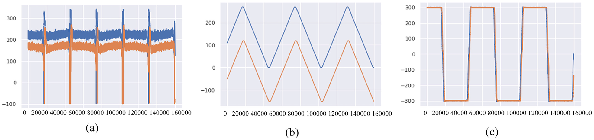
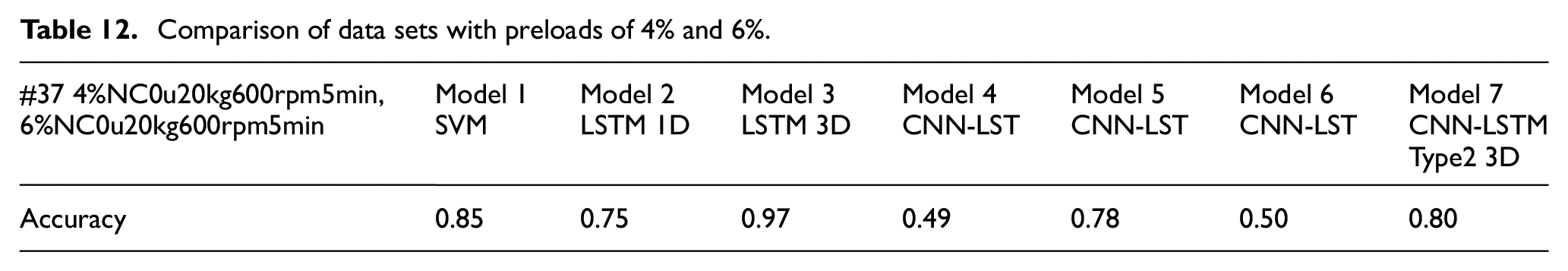
Figure 20 presents the current, position, and rpm plots for preloads of 4% (orange) and 6% (blue) based on experiment 37. The start-and-end positions for the 4% and 6% preloads varied because the hollow ball screw in the feed drive system had to be replaced. Therefore, the initial condition of the linear scale was different for each ball screw. Nevertheless, the recorded data for the repetitive motion of the ball screw (Figure 20(b)) were the same. For the 6% preload, oversized balls were used in the single-nut ball screw. The acquired signals were feed-forward and -backward signals containing information regarding the peak servo current associated with the linear scale signals. Differences between the changes in current and linear can be seen in the figure. The network was able to learn more effectively when more training data were available, and a deeper network could be used. Therefore, the 3D LSTM had higher accuracy than that of the 1D SVM (current). The SVM inputs were obtained through data mining, extension of the dimensionality of the raw data, and extraction of features to improve data preprocessing; these steps contributed to the SVM accuracy.³⁸ The accuracies of the 1D LSTM, 1D Type-1 CNN–LSTM, and 1D Type-2 CNN–LSTM models were 0.75, 0.49, and 0.50, respectively. Among these, the 1D LSTM had the highest accuracy; the CNN–LSTM architecture was unsuitable for this classification task because of subsampling and blurred filter effects. The accuracy of the 3D LSTM model was 0.97, which was higher than that of the 1D LSTM model; the accuracy of the 3D Type-1 CNN–LSTM model was 0.78, which was higher than that of the 1D Type-1 CNN–LSTM model; the accuracy of the 3D Type-2 CNN–LSTM model was 0.8, which was higher than that of the 1D Type-2 CNN–LSTM model (Table 11). These results indicate that for LSTM and CNN–LSTM models, a 3D data set is preferable to a 1D data set for updating the neural network parameters. The accuracy was higher when expensive linear scale equipment was used. However, for the 1D and 3D data sets, the accuracies of the Type-1 and Type-2 CNN–LSTM models did not differ substantially, indicating that the additional CNN layer in the Type 2 CNN–LSTM did not improve the accuracy (Table 12).

Figure 20.

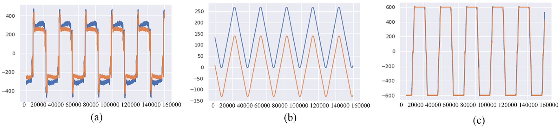
(a) Current, (b) position, and (c) rpm for experiment 37.

Table 12.

Comparison of data sets with preloads of 4% and 6%.

#37 4%NC0u20kg600rpm5min,6%NC0u20kg600rpm5min	Model 1	Model 2	Model 3	Model 4	Model 5	Model 6	Model 7
#37 4%NC0u20kg600rpm5min,6%NC0u20kg600rpm5min	SVM	LSTM 1D	LSTM 3D	CNN-LST	CNN-LST	CNN-LST	CNN-LSTM Type2 3D
Accuracy	0.85	0.75	0.97	0.49	0.78	0.50	0.80

Experiment 28: Details of prediction accuracy by each model’s performance

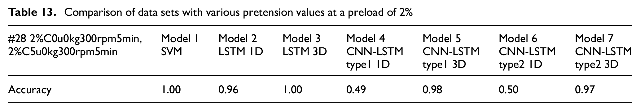
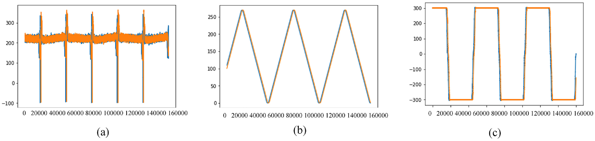
Figure 21 presents the current, position, and rpm plots for the 2%, C, 0 µm, 0 kg, 300 rpm, and 5 min (orange) and 2%, C, 5 µm, 0 kg, 300 rpm, and 5 min (blue) data sets. The position difference of the ball screw caused by thermal expansion can deteriorate the positioning accuracy of the feed drive system. Pretension is typically applied to the ball screw to compensate for thermal elongation. The loss of ball screw pretension results in a positioning error before the controller is used. In addition, through the application of FE in machine learning, the current signal was used to effectively obtain features for SVM training, yielding a classification accuracy of up to 100%. For deep learning, the current, rpm, and linear scale signals provided good synergy for feature extraction; thus, the 3D LSTM also yielded a classification accuracy of 100%. Moreover, the accuracies of the 3D Type-1 CNN–LSTM and 3D Type-2 CNN–LSTM were 0.98 and 0.97, respectively, indicating that the LSTM, Type-1 CNN–LSTM, and Type-2 CNNL-LSTM architectures effectively extracted features from the 3D data set. Among the 1D models, Model 2 had the highest accuracy (0.96), indicating that it effectively extracted features from the 1D (current) data set. By contrast, the accuracies of Models 4 and 6 were 0.49 and 0.5, respectively (Table 13). These results indicate that including a CNN architecture without using 2D image-like features does not yield effective feature extraction and distorts the data before they have been input into the LSTM layer.

Figure 21.

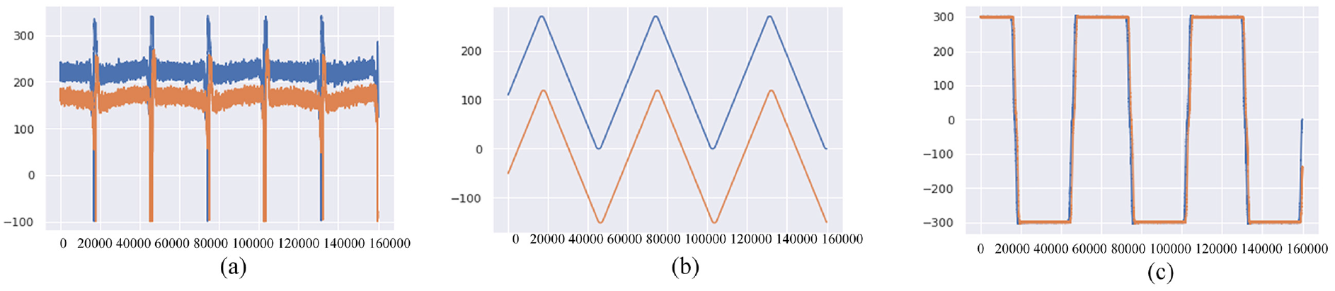
(a) Current, (b) position, and (c) rpm for experiment 28.

Table 13.

Comparison of data sets with various pretension values at a preload of 2%

#28 2%C0u0kg300rpm5min,2%C5u0kg300rpm5min	Model 1	Model 2	Model 3	Model 4	Model 5	Model 6	Model 7
#28 2%C0u0kg300rpm5min,2%C5u0kg300rpm5min	SVM	LSTM 1D	LSTM 3D	CNN-LSTM type1 1D	CNN-LSTM type1 3D	CNN-LSTM type2 1D	CNN-LSTM type2 3D
Accuracy	1.00	0.96	1.00	0.49	0.98	0.50	0.97

Experiment 24: Details of prediction accuracy by each model’s performance

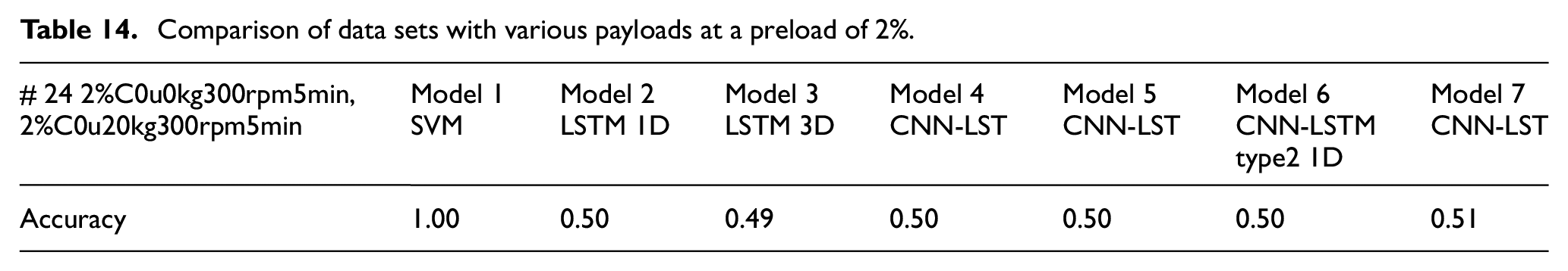
Figure 22 presents the current, position, and rpm plots for payloads of 0 kg (orange) and 20 kg (blue). The current signals did not differ substantially because the payload was compensated for by the support of the table’s linear guide. Therefore, the torque current of the motor exhibited the same trend during the motion of the CNC table, regardless of the payload. Variations in the current and position signals, as shown in Figures 22(a) and 22(b), were minimal. Because the deep learning models could not obtain suitable features, the accuracies of these models were not high. As indicated in Table 14, these models yielded accuracies of approximately 0.5. This is because the 2% preload condition resulted in preload loss, which increased mechanical backlash, increased the pitted ball trace, reduced stiffness, and introduced oscillatory position errors. The application of an oil-cooling system to the hollow ball screw to compensate for thermal rigidity in the current variation had limited effects. Without pretension, the positioning accuracy did not improve; therefore, an experimental time of 5 min was insufficient for deep learning in the 3D LSTM model. Thus, considering experiments 28 and 24, ball screw pretension dominates in industrial practice for thermal rigidity and positioning accuracy compensation. To classify the health of ball screws through feature extraction, pretention is essential, but oil-cooling is unnecessary. Accordingly, the classification accuracies of Models 2, 3, and 7 were higher in experiment 28 than in experiment 24.

Figure 22.

(a) Current, (b) position, and (c) rpm for experiment 24.

Table 14.

Comparison of data sets with various payloads at a preload of 2%.

# 24 2%C0u0kg300rpm5min,2%C0u20kg300rpm5min	Model 1	Model 2	Model 3	Model 4	Model 5	Model 6	Model 7
# 24 2%C0u0kg300rpm5min,2%C0u20kg300rpm5min	SVM	LSTM 1D	LSTM 3D	CNN-LST	CNN-LST	CNN-LSTM type2 1D	CNN-LST
Accuracy	1.00	0.50	0.49	0.50	0.50	0.50	0.51

Conclusions

Given the trends of big data, the Internet of Things, and smart manufacturing, smart analytics can be used to determine the health statuses of CNC machines. This study investigated the acquisition of large volumes of sensor data and data-driven approaches for evaluating machine health status. Since data cleaning and FE are required for fast computing to provide effective machinery prognostics. This study applied ANNs to classify the health of ball screws by using physics-based domain knowledge and data-driven prognostic deep learning models. Data sets of servo motor current, servo motor rpm, and optical linear scale were directly applied to perform prognostic classifications.

In summary, FE and Fisher’s score for the optical liner scale and the rpm of a ball screw feed drive system resulted in low classification accuracy, and these features were unsuitable for deployment in conventional machine learning models such as SVMs. For deep learning, training with a 3D data set (current, optical linear scale, and rpm) yielded higher accuracy than did training with a 1D data set (current). Therefore, data that are unrepresentative according to FE analysis may be useful in deep learning. All the raw data were used as inputs in the 3D LSTM model. Moreover, we trained and tested seven models with 37 data sets. In most cases, the accuracy of the SVM was higher than that of deep learning models. The maximum accuracy of the 3D LSTM model was close to that of the 1D SVM, but other deep neural networks performed poorly. Nevertheless, the 3D LSTM model had a higher accuracy than that of the 1D LSTM (current). Indeed, using expensive linear scale equipment improved the accuracy. The inputs of the SVM were obtained through data mining to extend the dimensionality of the raw data and abstract features. Finally, the experiments revealed that including an additional CNN layer in the CNN–LSTM architecture did not improve the classification accuracy. The subsampling and filtering of the CNN layer resulted in morphological effects, which reduced the effectiveness of the LSTM layer, even with an experimental time of 60 min. Overall, the performance of the deep learning networks was not as high as that of the SVM. This is because deep learning requires more training samples and more parameter updates. In addition, obtaining such large data sets is challenging in the health diagnosis of ball screws. This study investigated the advantages of using a deep learning model without feature extraction relative to those of supervised fine-tuned SVM learning. Base on the power of edge computing (EC), the real implement for fault classification with proposed model is promising and can be deployed successfully in the near future.

Footnotes

Declaration of conflicting interests

The author(s) declared no potential conflicts of interest with respect to the research, authorship, and/or publication of this article.

Funding

The author(s) disclosed receipt of the following financial support for the research, authorship, and/or publication of this article: The authors thanks the Ministry of Science and Technology for financially supporting this research under Grant MOST 109-2221-E-018-001-MY2 in part.

ORCID iD

Yi-Cheng Huang

References

Wei

Lin

Horng

. Analysis of a ball screw with a preload and lubrication. Tribol Int 2009; 42(11): 1816–1831.

Cuttino

Dow

Knight

. Analytical and experimental identification of nonlinearities in a single-nut, preload ball screw. J Mech Des 1997; 119: 15–19.

Peng

Tse

Chu

. A comparison study of improved hilbert–huang transform and wavelet transform: application to fault diagnosis for rolling bearing. Mech Syst Signal Process 2005; 19: 974–988.

Zhang

Zhou

, et al. Positioning error prediction and compensation of ball screw feed drive system with different mounting conditions. Proc IMechE, Part B: J Engineering Manufacture 2016; 230(12): 2307–2311.

Zhao

Zhang

. Adaptive on-line compensation model on positioning error of ball screw feed drive systems used in computerized numerical controlled machine tools. Proce IMechE, Part B: J Engineering Manufacture 2019; 233(3): 914–926.

Wang

Vachtsevanos

. Fault prognosis using dynamic wavelet neural networks. Artif Intell Eng Des Anal Manuf 2001; 15: 349–365.

Tsai

Cheng

Hwang

. Ball screw preload loss detection using ball pass frequency. Mech Syst Signal Process 2014; 48: 77–91.

Bacha

Salem

Chaari

. An improved combination of Hilbert and Park transforms for fault detection and identification in three-phase induction motors. Int J Electr Power Energy Syst 2012; 43: 1006–1016.

Huang

Zheng

. Ball nut preload diagnosis of the hollow ball screw through support vector machine. Adv Technol Innov 2018; 3(2): 94.

10.

Wang

Zhang

. Automatic blur type classification via ensemble SVM. Signal Process Image Commun 2019; 71: 24–35.

11.

Patel

Upadhyay

. Comparison between artificial neural network and support vector method for a fault diagnostics in rolling element bearings. Procedia Eng 2016; 144: 390–397.

12.

Liu

Choo

KKR

Wang

, et al. SVM or deep learning? A comparative study on remote sensing image classification. Soft Comput 2017; 21(23): 7053–7065.

13.

Lee

Zhao

, et al. Prognostics and health management design for rotary machinery systems-Reviews, methodology and applications. Mech Syst Signal Process 2014; 42: 314–334.

14.

, et al. Machine vision and deep learning based rubber gasket defect etection. Adv Technol Innov 2020, 5(2): 76.

15.

Hochreiter

Jürgen

. LSTM can solve hard long time lag problems. In: Proceedings of the advances in neural information processing systems, Denver, CO, USA, 2–5 December 1996, pp.473–479. New York, NY: IEEE.

16.

Ribeiro

Neto

PSDM

Cavalcanti

, et al. Lag selection for time series forecasting using particle swarm optimization. In: Proceedings of the IEEE 2011 international joint conference on neural networks (IJCNN), San Jose, CA, USA, 31 July–5 August 2011, pp.2437–2444. New York, NY: IEEE.

17.

LeCun

Bengio

Hinton

. Deep learning. Nature 2015; 521: 436.

18.

Wang

Zhuang

Duan

, et al. A multi-scale convolution neural network for featureless fault diagnosis. In: Proceedings of the 2016 international symposium on flexible automation (ISFA), Cleveland, OH, USA, 1–3 August 2016, pp.65–70.

19.

Ren

Sun

Wang

, et al. Prediction of bearing remaining useful life with deep convolution neural network. IEEE Access 2018; 6: 13041–13049.

20.

Sateesh

Babu G

Zhao

. Deep convolutional neural betwork based regression approach for estimation of remaining useful life. In database systems for advanced applications. In Navathe

Shekhar

, et al. (eds) International conference on database systems for advanced applications. Cham: Springer, 2016, pp.214–228.

21.

Zhang

Wang

Yan

, et al. Long short-term memory for machine remaining life prediction. J Manuf Syst 2018; 48: 78–86.

22.

Zheng

Ristovski

Farahat

, et al. Long short-term memory network for remaining useful life estimation. In: Proceedings of the 2017 IEEE international conference on prognostics and health management (ICPHM), Dallas, TX, USA, 19–21 June 2017, pp.88–95. New York, NY: IEEE.

23.

Zhang

Wang

, et al. Layerwise perturbation-based adversarial training for hard drive health degree prediction. In: Proceedings of the 2018 IEEE international conference on data mining (ICDM), Singapore, 17–20 November 2018, pp.1428–1433. New York, NY: IEEE. New York, NY: IEEE.

24.

Guo

Jia

, et al. A recurrent neural network based health indicator for remaining useful life prediction of bearings. Neurocomputing 2017; 240: 98–109.

25.

Wang

Lai

, et al. Dimensional sentiment analysis using a regional CNN-LSTM model. In: Proceedings of the 54th annual meeting of the association for computational linguistics, Berlin, Germany, 7–12 August 2016, pp.225–230. Stroudsburg, PA: Association for Computational Linguistics.

26.

Sainath

Vinyals

Senior

, et al. Convolutional, long short-term memory, fully connected deep neural networks. In: Proceedings of the 2015 IEEE international conference on acoustics, speech and signal processing (ICASSP), Brisbane, Australia, 19–24 April 2015, pp.4580–4584. New York, NY: IEEE.

27.

Ullah

Ahmad

Muhammad

, et al. Action recognition in video sequences using deep bi-directional LSTM with CNN features. IEEE Access 2018; 6: 1155–1166.

28.

Tan

, et al. Automated diagnosis of arrhythmia using combination of CNN and LSTM techniques with variable length heart beats. Comput Biol Med 2018; 102: 278–287.

29.

Zhao

Yan

Wang

, et al. Learning to monitor machine health with convolutional bi-directional LSTM networks. Sensors 2017; 17: 273.

30.

Yue

Ping

Lanxin

. An end-to-end model based on CNN-LSTM for industrial fault diagnosis and prognosis. In: Proceedings of the 2018 International Conference on Network Infrastructure and Digital Content (IC-NIDC), Guiyang, China, 22–24 August 2018, pp.274–278. New York, NY: IEEE.

31.

Kim

Cho

. Predicting residential energy consumption using CNN-LSTM neural networks. Energy 2019; 182: 72–81.

32.

Cortes

Vapnik

. Support-vector networks. Mach Learn 1995; 20: 273–297.

33.

Boser

Guyon

Vapnik

. A training algorithm for optimal margin classifiers. In: Proceedings of the fifth annual workshop of computational learning theory, Pittsburgh, PA, USA, 27–29 July 1992, vol. 5, pp.144–152. New York, NY: ACM.

34.

Bishop

Jordan

Kleinberg

, et al. Pattern recognition and machine learning. New York, NY: Springer, 2006, pp.1–4.

35.

Qiu

Lee

. Feature fusion and degradation detection using self-organizing map. In: Proceedings of the 2004 international conference on machine learning and applications, Louisville, KY, USA, 16–18 December 2004, pp.107–114. New York, NY: IEEE.

36.

Casoetto

Djurdjanovic

Mayor

, et al. Multisensor process performance assessment through use of autoregressive modeling and feature maps. J Manuf Syst 2003; 22: 64–72.

37.

Jin

Chen

Lee

. Methodology for ball screw component health assessment and failure analysis. In: Proceedings of the ASME 2013 international manufacturing science and engineering conference collocated with the 41st North American manufacturing research conference, Volume 2: Systems; Micro and nano technologies; Sustainable manufacturing, Madison, WI, USA, 10–14 June 2013, V002T02A031. New York, NY: ASME.

38.

Huang

Hsieh

. Applying a support vector machine for hollow ball screw condition-based classification using feature extraction. Proc IMechE Part B: J Engineering Manufacture. Epub ahead of print 14 October 2020. DOI: 10.1177/0954405420958842

39.

Colah.github.io. Understanding LSTM networks—Colah’s blog, http://colah.github.io/posts/2015-08-Understanding-LSTMs (2018, accessed on 5 April 2018)

40.

Patterson

Gibson

. Deep learning. A practitioner’s approach. Sebastopol, CA; O’Reilly Media, Inc, 2017, pp.150–158.

41.

Kingma

. Adam: a method for stochastic optimization. arXiv 2014, arXiv:1412.6980

A revisit for the diagnosis of the hollow ball screw conditions based classification using deep learning

Abstract

Keywords

Introduction

Methods

Support vector machines

Feature engineering

Convolutional neural network

RNN and LSTM-RNN

Hybrid CNN architecture

Results

Experimental design

Neural network parameters and hyperparameter experiments

LSTM network parameters and hyperparameter experiments

LSTM network parameter experiment

LSTM network hyperparameter experiment

LSTM accuracy with 1D, 2D, and 3D data sets

Type-1 CNN–LSTM network parameters and hyperparameter experiments

Type-1 CNN–LSTM network parameter experiment

Type-1 CNN–LSTM network hyperparameter experiment

Type-1 CNN–LSTM accuracy with 1D, 2D, and 3D data sets

Type-2 CNN–LSTM network parameters and hyperparameter experiments

Type-2 CNN–LSTM network parameter experiment

Type-2 CNN–LSTM

Type-2 CNN–LSTM accuracy with 1D, 2D, and 3D data sets

Comparison of the LSTM, Type-1 CNN–LSTM, and Type-2 CNN–LSTM networks with different data sets

Neural network comparison

Discussion

Experiments 1–20: Applications for the standard 4% preload ball screw

Experiments 21–23 and 36–37: Comparisons for the 2% preload loss with standard 4% preload ball screw

Experiments 24–29: 2% preload loss ball screw under the circumstances of applying oil cooling system

Experiments 30–35: Comparison for the standard 4% preload and more rigidity 6% preload ball screws

Experiment 37: Details of prediction accuracy by each model’s performance

Experiment 28: Details of prediction accuracy by each model’s performance

Experiment 24: Details of prediction accuracy by each model’s performance

Conclusions

Footnotes

Declaration of conflicting interests

Funding

ORCID iD

References