Sage Journals: Discover world-class research

Abstract

Transients in hydropower plants can result in serious disturbances in a plant operation and damage of mechanical and civil components. The best way to prevent such adverse outcomes is to conduct a transient-state analysis using a mathematical model of the hydropower plant system. Based on the collected data on 270 hydropower plants with cross-flow turbines, regression equations were derived that relate a cross-flow turbine specific speed, rated speed, runner diameter and runner width to the rated turbine head and discharge. The obtained equations were used to estimate the turbine performance characteristics using available unit hill charts of three different cross-flow turbines. Finally, the estimated performance characteristics were used to form the boundary condition ‘cross-flow turbine’ within the unsteady 1D mathematical model. The model was validated through case studies by comparing calculated and measured changes in the turbine speed and inlet pressure, induced by sudden load rejection. The difference between the calculated and measured peak pressures was up to 5% during the most critical period, that is, from the moment of load rejection up to the guide vanes closure. In the case of turbine speed, the difference between the peak values was less than 10% in the same period.

Keywords

Cross-flow turbine unit characteristics hill chart hydropower plant load rejection transients water hammer

Introduction

Operation of a hydraulic system can be steady or unsteady (e.g. transient). While the steady-state operation is characterised by constant flow over time, the transient regimes are characterised by dynamic changes in pressure and flow in the system. Unsteady flow also results in dynamic change of flow dependent hydraulic parameters such as pipe friction factor (see e.g. Riasi et al.¹).

The intensity of transient-state pressure changes closely depends on the flow velocity change, but also on numerous system parameters such as pipe length and diameter, pipe material, compressibility of water, gas content in water, characteristics of valves and hydraulic machines involved, etc. In some cases, the increase or decrease in pressure can be so intense that it causes serious damage within the system, that is, a burst of system parts.

Transient regimes in hydraulic systems can be triggered by various events which could be divided into two major groups: uncontrolled/unintentional events (e.g. sudden power failure) and controlled events (e.g. hydraulic machine start-up or shutdown, change in speed of hydraulic machine, change in control valve opening, etc.). In both cases, the safety of a system must be considered and adequate preventive measures must be provided in advance.

A good example of the complexity of transients in hydraulic systems is the study by Garg and Kumar² on water hammer in pipelines made of different materials. They have calculated and measured lower water hammer pressures in pipeline made of Glass Reinforced Fibre Plastic (GRP) compared to pipeline made of a combination of GRP and Mild Steel (MS) and significantly lower water hammer pressures compared to pipeline fully made of MS.

A hydropower plant is generally considered a complex hydraulic system. The transient regimes in hydropower plants occur mainly due to changes in the turbine operation or due to changes in the inlet valve opening. The research presented in this paper is focused on the transients generated by changes in the turbine operation, particularly sudden load rejection.

Transients in hydropower plants and in hydraulic systems in general have been the subject of research by numerous researchers for a long time. The first published results related to the subject of water hammer date back to the beginning of the 20th century (Joukowsky³; Allievi⁴). Over time, extensive research efforts have resulted in the partial standardisation of certain parameters that characterise unsteady operation of hydropower plants and in the formation of IEC standards used worldwide today (e.g. IEC 60308⁵). However, despite attempts to standardise the construction and operation of hydropower plants, each hydropower plant is still a unique facility whose behaviour depends on a large number of parameters, especially in transient-state regimes.

Besides the parameters that generally affect the transient-state operation of any hydraulic system (i.e. pipe material, diameter, length, friction, etc.), in the case of a hydropower plant some system specific parameters must be considered. These include performance characteristics of the installed turbines and flow characteristics of the inlet valves (see e.g. Kodura⁶), but also the closing law of the turbine flow control assemblies, such as Pelton turbine nozzles (see e.g. Bergant et al.⁷) or Francis turbine guide vanes (see e.g. Zhang et al.⁸).

Hydraulic turbine is the heart of a hydropower plant, hence its type and performance characteristics (e.g. hill charts) deserve special attention in transient-state analyses. However, despite the plentiful data published in professional and scientific literature regarding the Francis, Pelton or Kaplan turbines, the available data on the steady-state and especially transient operation of the cross-flow turbines are still very limited.

Cross-flow (Ossberger, Banki-Michell) turbine is a low-speed, impulse type turbine. Unlike most water turbines, which have axial or radial flows, in a cross-flow turbine the water passes through the turbine transversely, or across the turbine blades.⁹

In practice, cross-flow turbines are mostly used in the net head range from 2.5 to 200 m and in the flow range from 0.04 to 13 m³ s⁻¹ (Adhikari¹⁰; AHEC-IITR¹¹; Ossberger Hydro¹²). Cross-flow turbines are one of the cheapest and most robust turbines that are increasingly used in small hydropower plants due to their simple design, good technical performance and high adaptability to flow changes, especially if the turbine is built as a two-cell unit (usually in 2:1 ratio).

A turbine is generally the part of a hydropower system that is the most difficult to model mathematically. The flow through the turbine is extremely complex, spatial, unsteady, non-uniform and sometimes multiphase (mixture of water, vapour and air). Even in steady-state operation, the turbine flow is prone to instabilities that may arise from various turbine specific phenomena such as leakage vortices induced by tip clearance between the runner and shroud (Ma et al.¹³) or draft tube swirl (Zhou et al.¹⁴). During transient regimes, the situation becomes more complicated since the turbine speed is variable due to the torque imbalance on the runner.

Modern CFD techniques are certainly a powerful and widely used tool for analysing the flow in turbines, assessing their performance characteristics and predicting their behaviour under different operating conditions. Cross-flow turbines are no exception, as evidenced by numerous published scientific papers based on application of the CFD for the analysis, development and design of this type of turbine. One of the latest advances in this field has been reported by Mehr et al.¹⁵ They have used a commercial CFD software to develop a three-step numerical method for a cross-flow turbine nozzle design (first step), runner optimisation (second step) and turbine performance enhancement (third step). Such an approach enabled them to optimise the turbine design in order to achieve increased efficiency, assess the turbine performance characteristics and analyse the turbine performance under different load conditions. Potentially, if coupled with a common 1D model of unsteady flow in pipes, such a CFD model of a cross-flow turbine could provide a comprehensive tool for analysing transient operation of hydropower plants. In the case of Francis turbines, similar method has already been proposed by Zhang et al.⁸ However, in the case of cross-flow turbines such an attempt has not yet been published.

On the other hand, all CFD methods require that the internal geometry of the turbine is known or assessed in advance. In this paper, a different, simpler approach for predicting cross-flow turbine behaviour during transient operation is proposed. This method requires only the rated or design net head and discharge of the turbine to be known. No information on the turbine design is needed in advance, which should enable this method to be used in the design stage of hydropower plants. As far as the authors are aware, such an approach has not yet been published in the available literature.

The presented method uses new empirical equations that relate a cross-flow turbine specific speed, rated speed, runner diameter and runner width to the rated turbine head and discharge. These equations were derived using regression analysis of the collected data on 270 hydropower plants with cross-flow turbines. The obtained regression equations were then used to estimate the turbine performance characteristics based on the available unit hill charts of three different cross-flow turbines. Finally, the obtained performance characteristics were used to form the boundary condition ‘cross-flow turbine’ within the 1D mathematical model of unsteady operation of hydropower plants.

Method statement

Cross-flow turbine characteristics

In the transient regime, it is important to consider flow and pressure changes in the system over time. In case the transient regime is triggered by changes in the turbine operation, the hydraulic response of the system depends not only on the opening/closing time of the turbine guide vanes (or wicket gate) but also on the (variable) runner speed.

To understand the behaviour of a turbine in transient regimes, its performance characteristics must be known in advance. These characteristics include the relationships between speed n, discharge Q, head H, torque T, power P, opening of the guide vanes – and in the case of Kaplan turbines – the angle of the runner blades ϕ. Most of the above characteristics are usually represented in the form of unit hill charts in which the so-called unit quantities refer to the turbine having runner diameter of 1 m and operating at 1 m net head (Jordan,¹⁶ Benišek,¹⁷ Kovalev¹⁸):

Unit speed : n_{11} = \frac{n D}{\sqrt{H}}

(1)

Unit discharge : Q_{11} = \frac{Q}{D^{2} \sqrt{H}}

(2)

Unit power : P_{11} = \frac{P}{D^{2} H^{1.5}} = g Q_{11} η

(3)

where the rotational speed n should be given in min⁻¹, runner diameter D and turbine net head H in m and power in kW.

Unit speed n₁₁, discharge Q₁₁ and power P₁₁ are commonly associated with units min⁻¹, m³ s⁻¹ and kW respectively, although their actual dimensions are quite different and have no physical meaning.

Turbine performance characteristics are generally obtained by testing a down-scaled model on the manufacturer’s test rig. The results of such model tests are usually given in the form of n₁₁–Q₁₁ hill charts that represent relationships between unit flow Q₁₁, unit speed n₁₁, and efficiency η, in function of guide vane or wicket gate opening φ.

One of the most important parameters, widely used in the theory and practice of turbomachinery, is the specific speed n_s. In the case of hydraulic turbines, it is defined (old IEC formula) as the speed of a geometrically similar turbine which would produce power of 1 kW under the net head of 1 m:

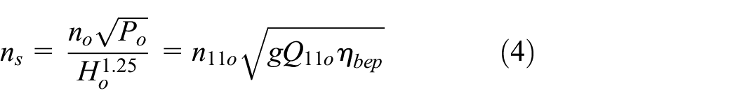
n_{s} = \frac{n_{o} \sqrt{P_{o}}}{H_{o}^{1.25}} = n_{11 o} \sqrt{g Q_{11 o} η_{b e p}}

(4)

where the n_o, P_o, and H_o or n_11o and Q_11o refer to the best efficiency point η = η_bep.

Specific speed n_s is formally considered to be a dimensionless quantity, although it has some (meaningless) dimension according to equation (4). Specific speed is used for classification, comparison, and scaling of turbines, but also as a starting point in the sizing of a turbine and estimating its performance characteristics, if these characteristics are not known.

In the case of cross-flow turbines, the lack of their performance characteristics (e.g. hill charts) is the rule since the turbine manufacturers generally avoid providing them. This is a serious problem that practically makes it impossible to analyse the operation of a turbine, especially in transient regimes. Moreover, in the design stage of a hydropower plant, where it is necessary to analyse both steady-state and transient operation of the plant, the only reliable data available to the designer are the required design head and discharge of the turbine.

In the following text, new equations are proposed that relate specific speed, rated speed, and the runner diameter and width to the known rated or design head and discharge of an arbitrary cross-flow turbine. Based on these equations, the linear interpolation method was applied to estimate the unit performance characteristics of that turbine by using known unit hill charts of three different cross-flow turbines.

In practice, the specific speed is calculated in the first iteration, using empirical equations based on the known turbine head. The turbine rated or design head is generally used in these equations, assuming it is equal to the head at the best efficiency point. One such empirical equation, proposed by Kpordze and Warnick¹⁹ is given as:

n_{s} = \frac{513.846}{H^{0.5047}}

(5)

Equation (5) is applicable to the cross-flow turbines and was derived using regression analysis of the basic data on 17 different cross-flow turbines.

For the purpose of the research presented in this paper, the basic data (rated speed, head, discharge, shaft power, runner diameter and width) for 270 cross-flow turbines were collected. The selected turbines have been installed in small hydropower plants all over Europe in the period from 2006 to 2019.

The collected data were processed by nonlinear regression analysis. As the first result, two regression equations for the specific speed were derived as follows:

n_{s} (H) = \frac{323.61325}{H^{0.38151}}; (R^{2} = 0.69)

(6)

n_{s} (H, Q) = 315.2615 \frac{Q^{0.09467}}{H^{0.37802}}; (R^{2} = 0.7)

(7)

where R² is the coefficient of determination.

Equation (6) relates the specific speed of a cross-flow turbine to the known rated head of the turbine, while equation (7) relates the specific speed to the known rated head and discharge.

Figure 1(a) shows the scattering of the specific speeds of all sample cross-flow turbines, calculated using equation (4), with respect to the regression curve n_s(H), obtained using equation (6). For comparison, the n_s(H) curve according to equation (5) is also plotted. Figure 1(b) shows specific speeds n_s of the sample turbine units versus turbine speed n_s(H, Q) calculated using equation (7). The straight line in Figure 1(b) refers to the calculated specific speeds n_s= n_s(H, Q).

Figure 1.

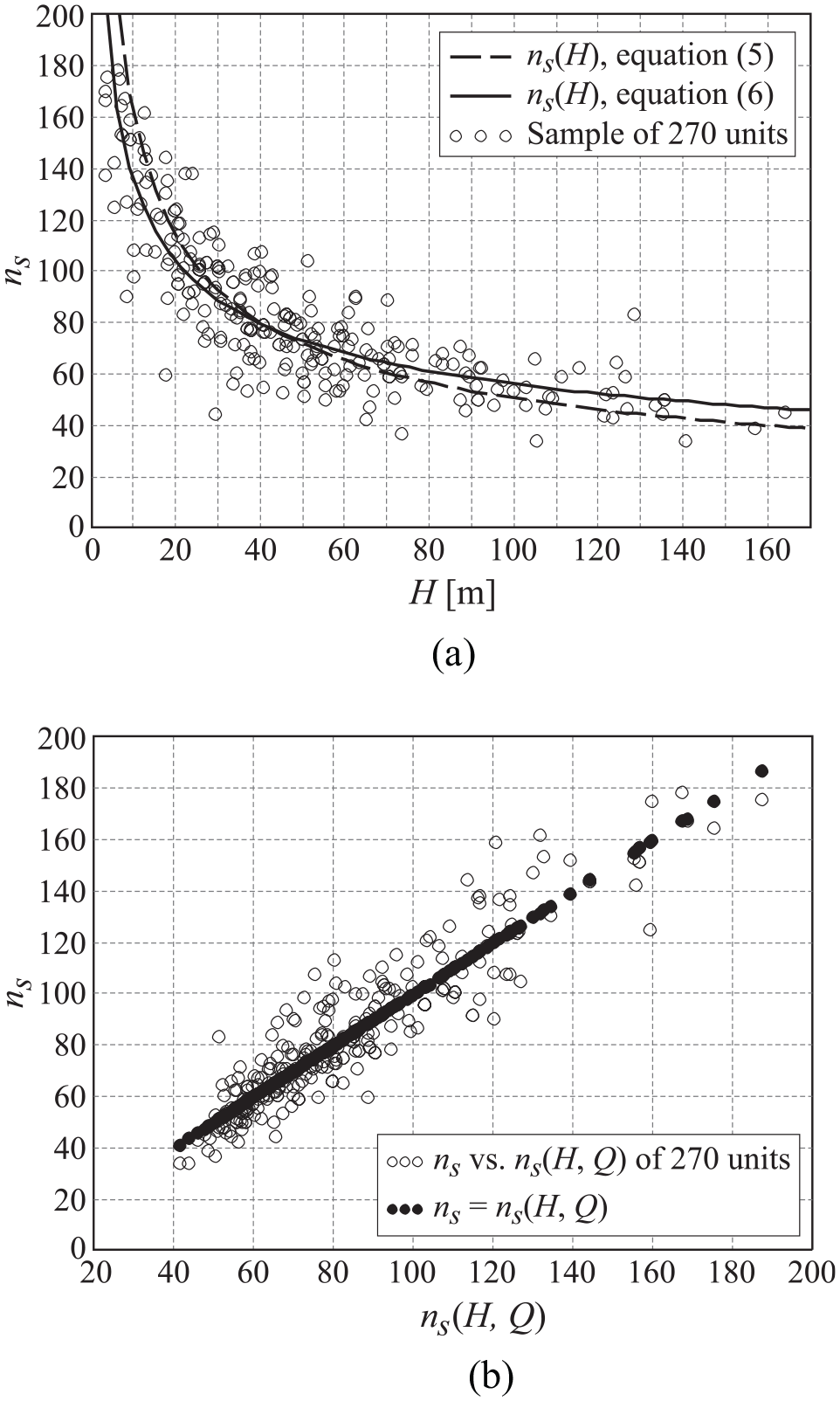
Specific speed n_s of cross-flow turbines: (a) specific speed n_s versus rated net head H and (b) actual specific speed n_s versus calculated n_s(H, Q).

As it can be inferred from the results given in Figure 1, both regression equations (6) and (7) show very good reliability in estimating the turbine specific speed. Both equations may be used separately or simultaneously, in which case the mean value should be taken as the final result.

For the known specific speed n_s, the turbine rated speed n_o may be assessed using equation (4), by substituting P = ρgQHη and assuming the cross-flow turbine efficiency in the range of η = 0.75–0.85. To avoid efficiency estimation, two new regression equations for the turbine speed were derived based on the collected data on 270 cross-flow turbines:

n_{o} = n_{HQ} (H, Q) = 114.846 \frac{H^{0.36025}}{Q^{0.40679}}; (R^{2} = 0.88)

(8)

n_{o} = n_{HD} (H, D) = 35.386 \frac{H^{0.53012}}{D^{1.00601}}; (R^{2} = 0.95)

(9)

Equation (8) relates the speed of a cross-flow turbine to the known rated head and discharge, while equation (9) relates the turbine speed to the rated head and the runner diameter, assuming the latter is known or selected in advance.

In order to get an impression of the collected data dispersion, Figure 2(a) shows the actual rated speeds n_o of the sample turbine units versus turbine speeds n_HQ(H, Q) calculated using equation (8). The straight line in Figure 2(a) stands for the calculated speeds n_o= n_HQ(H, Q). Figure 2(b) has the same meaning but refers to equation (9).

Figure 2.

Rated speed n_o of cross-flow turbines: (a) actual rated speed n_o versus calculated speed n_o(H, Q) and (b) actual rated speed n_o versus calculated speed n_o(H, D).

The given results show high reliability of regression equations (8) and (9), particularly in the lower rotational speed range (lower than 500 min⁻¹), where the deviations are negligible. In the higher speed range, the deviations are more significant, but obviously because the actual turbine speeds are mostly equal to the synchronous speeds of the electric generator. In other words, higher speed cross-flow turbines are usually directly coupled with their generator, while low-speed turbines generally require the installation of some kind of speed increaser between the turbine and the generator. Hence, in case the turbine needs to be directly coupled with the electric generator (mostly for n_o ≥ 500 min⁻¹), the result of equation (8) or equation (9) should be rounded to the closest synchronous speed of rotation.

Using the same sample data and the same methodology, two more regression equations were derived that relate the runner diameter and width to the rated head and discharge:

D = D_{HQ} (H, Q) = 0.3107 H^{0.16868} Q^{0.39962}; (R^{2} = 0.94)

(10)

B = B_{HQ} (H, Q) = 3.5993 \frac{Q^{0.63989}}{H^{0.58729}}; (R^{2} = 0.92)

(11)

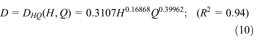
Figure 3(a) presents actual runner diameters D of the sample turbine units in relation to the diameters D(H, Q) calculated using regression equation (10). The straight line stands for the calculated diameters D = D(H, Q). Figure 3(b) has the same meaning but is related to the runner width and regression equation (11).

Figure 3.

Basic runner dimensions of cross-flow turbines: (a) actual runner diameter D versus calculated diameter D_HQ(H, Q) and (b) actual runner width B versus calculated width B_HQ(H, Q).

The obtained results show very good agreement and high reliability, especially in the case of equation (11), which is aimed for estimation of a cross-flow turbine runner width. In the case of the runner diameter, it should be noted that all the diameters of the actual turbines are rounded to (manufacturer’s) standard values (200, 300, 400 mm, and so on). A similar procedure may be applied when using equation (10), that is, the obtained result for the particular head and discharge could be rounded to the closest multiple of 50 or 100 mm.

Equations (6)–(11) enable assessment of the specific speed n_s, rated speed n_o, runner diameter D, and runner width B for the known rated or design head H_o and discharge Q_o of an arbitrary cross-flow turbine. The specific speed n_s is the starting parameter for assessment of the unit performance characteristics of the turbine, while the rated speed and the runner diameter are needed to calculate the turbine performance parameters (head, discharge, shaft power, torque, and speed of rotation) from the estimated unit characteristics.

The unit performance characteristics of a cross-flow turbine, for which only the design or rated head and flow are known, can be estimated if the unit hill charts for at least two cross-flow turbines of different specific speeds are known. For this purpose, the unit hill charts of three cross-flow turbines have been found in the literature and on the internet. The specific speeds of these turbines are n_s= 45.7, n_s = 68.8, and n_s = 93.4. The unit hill charts of the selected cross-flow turbines are given in Figure 4.

Figure 4.

Unit hill charts of three cross-flow turbines of different specific speeds: (a) cross-flow turbine B5-N, n_s = 45.7,²⁰ (b) cross-flow turbine B5N-GD-N1-x, n_s = 68.8 (Calov²¹), and (c) cross-flow turbine T15 n_s= 93.4.²²

The procedure for assessment of the unknown performance characteristics of an arbitrary cross-flow turbine is briefly described in five steps as follows.

Step 1. All three hill charts given in Figure 4 must be digitalised, that is, transformed into the dimensionless matrix form by introducing the following dimensionless unit quantities:

Q_{1} = \frac{Q_{11}}{Q_{11 o}}

(12)

n_{1} = \frac{n_{11}}{n_{11 o}}

(13)

P_{1} = \frac{P_{11}}{P_{11 o}}

(14)

where the unit quantities n_11o, Q_11o, and P_11o refer to the turbine best efficiency point.

At this point some assumptions must be made regarding the off-design regimes of a turbine. Namely, the unit hill charts given in Figure 4 cover only the regimes expected in normal that is, designed steady-state operation of the turbine. However, as noticed by Iovănel et al.,²³ due to the increasing instability of the energy market, hydropower plants frequently work at off-design parameters, even in steady-state regimes. When it comes to transient-state operation, for example, after sudden load rejection, the turbine always passes (albeit briefly) through the regimes that are outside the designed operating range. Therefore, the off-design operating regimes are particularly important from the aspect of mathematical modelling and analysis of a turbine behaviour during transient operation.

By analysing the performance characteristics of various cross-flow turbines that can be found in the literature (Durgin and Fay²⁴; Adhikari¹⁰; Mockmore and Merryfield²⁵), it can be concluded that the turbine unit performance characteristics on their left and right boundaries could be estimated as:

n ₁₁ ≈ 0 Q₁₁ ≈ 0 and P₁₁ ≈ 0.

n ₁₁ ≈ 2n_11oQ₁₁ ≈ 0 and P₁₁ ≈ 0.

By introducing these assumptions and applying the described procedure, each of the hill diagrams given in Figure 4 can be converted into a pair of equally sized matrices:

[Q_{1}^{T_{i}}]_{(m, n)} = f_{Q_{1}}^{T_{i}} (n_{1}^{T_{i}}, φ), i = 1, 2, 3

(15)

[P_{1}^{T_{i}}]_{(m, n)} = f_{P_{1}}^{T_{i}} (n_{1}^{T_{i}}, φ), i = 1, 2, 3

(16)

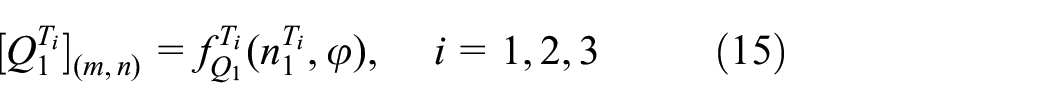
where the superscripts T₁, T₂, T₃ refer to the cross-flow turbines of known hill charts given in Figure 4 (hence $n_{s}^{T_{1}} = 45.7$ , $n_{s}^{T_{2}} = 68.8$ , and $n_{s}^{T_{3}} = 93.4$ ).

It should be noted that in matrices (15) and (16) the dimensionless unit speed n₁ is always in the range 0–2 while the opening of the guide vane φ is in the range 0–1.

Step 2. The specific speed $n_{s}^{T}$ of the considered cross-flow turbine (T) is calculated using equation (4), if all the rated quantities ( $n_{o}^{T}, P_{o}^{T}, H_{o}^{T}$ ) are known or using equation (6) or (7), if only the rated head and discharge are known.

Step 3. Out of the three available cross-flow turbines of known characteristics, two (for example T₁ and T₂) are selected whose specific speeds are $n_{s}^{T_{1}} < n_{s}^{T} < n_{s}^{T_{2}}$ .

The dimensionless unit characteristics of the considered cross-flow turbine (T) are calculated using linear interpolation:

(Q_{1}^{T})_{i, j} = \frac{n_{s}^{T} - n_{s}^{T_{1}}}{n_{s}^{T_{2}} - n_{s}^{T_{1}}} [{(Q_{1}^{T_{2}})}_{i, j} - {(Q_{1}^{T_{1}})}_{i, j}] + (Q_{1}^{T_{1}})_{i, j}

(17)

(P_{1}^{T})_{i, j} = \frac{n_{s}^{T} - n_{s}^{T_{1}}}{n_{s}^{T_{2}} - n_{s}^{T_{1}}} [{(P_{1}^{T_{2}})}_{i, j} - {(P_{1}^{T_{1}})}_{i, j}] + (P_{1}^{T_{1}})_{i, j}

(18)

where i = 1…m and j= 1…n.

In the case where $n_{s}^{T_{2}} < n_{s}^{T} < n_{s}^{T_{3}}$ , the superscripts T₁ and T₂ in equations (17) and (18) should be simply replaced with T₂ and T₃.

Step 4. Unit speed, unit discharge, and unit power at the best efficiency point of the considered cross-flow turbine ( $n_{11 o}^{T}, Q_{11 o}^{T}, P_{11 o}^{T}$ ) are calculated using equations (1)–(3). If not known, the turbine rated speed n_o can be assessed using equation (8) based on the rated head and discharge, while the runner diameter D can be assessed using equation (10).

Step 5 (final). The unit characteristics of the considered cross-flow turbine (T) in matrix form, are calculated as follows:

{[n_{11}^{T}]}_{m, 1} = n_{11 o}^{T} {[n_{1}^{T}]}_{m, 1}

(19)

{[Q_{11}^{T}]}_{m, n} = Q_{11 o}^{T} {[Q_{1}^{T}]}_{m, n}

(20)

{[P_{11}^{T}]}_{m, n} = P_{11 o}^{T} {[P_{1}^{T}]}_{m, n}

(21)

As an example, the final results of the above-described procedure are given in Figure 5 in form of unit charts Q₁₁–n₁₁ and P₁₁–n₁₁ in function of the guide vane opening φ. The presented results refer to a cross-flow turbine with the specific speed n_s = 65.6 (H_o = 85 m, Q_o = 4.5 m³s⁻¹, P_o = 3227 kW, n_o= 298 min⁻¹). This turbine is one of the three turbines whose transient-state operation has been analysed within the case studies presented in this paper.

Figure 5.

Calculated unit charts Q₁₁–n₁₁ and P₁₁–n₁₁ for cross-flow turbine with n_s= 65.6.

It should be emphasised that the hill charts used as the basis of the described procedure refer to the steady-state operation of the given cross-flow turbines. Hence, the resulting calculated turbine characteristics are also valid only for steady-state operation. However, according to Chaudry,²⁶ in the absence of data on transient turbine operation, it can be assumed that the turbine characteristics based on the steady-state model tests are also valid during the transient state.

Transient-state model of hydropower plants with cross-flow turbines

A hydropower plant system with a cross-flow turbine is mathematically modelled in the same way as any other pipe network, that is, as a set of nodes and links. The links represent the pipes between the nodes while the nodes represent the boundary conditions (tanks, junction of two or more pipes, turbines, valves, etc.).

Unsteady flow in pipelines that follows sudden changes in turbine operation, load rejection, motion of turbine guide vanes, closing or opening of inlet valves, etc., is usually described by the (simplified) continuity equation (22) and momentum equation (23) (Chaudry²⁶; Obradović²⁷):

\frac{\partial H}{\partial t} + \frac{a^{2}}{gA} \frac{\partial Q}{\partial t} = 0

(22)

\frac{\partial Q}{\partial t} + gA \frac{\partial H}{\partial x} + \frac{f}{2 dA} Q | Q | = 0

(23)

Equations (22) and (23) represent a pair of first-order hyperbolic partial differential equations. Coupled with the known boundary and initial conditions, these equations are commonly solved numerically using the method of characteristics. As a result, variations of flow Q(x, t) and head H(x, t) are obtained at discrete distance-time points along all pipes of the hydraulic system.

A general sketch of the hydropower plant with cross-flow turbine is given in Figure 6. The computational domain comprises penstock (2) and a short inlet pipe (1). All necessary boundary conditions (BC) are also marked in Figure 6.

Figure 6.

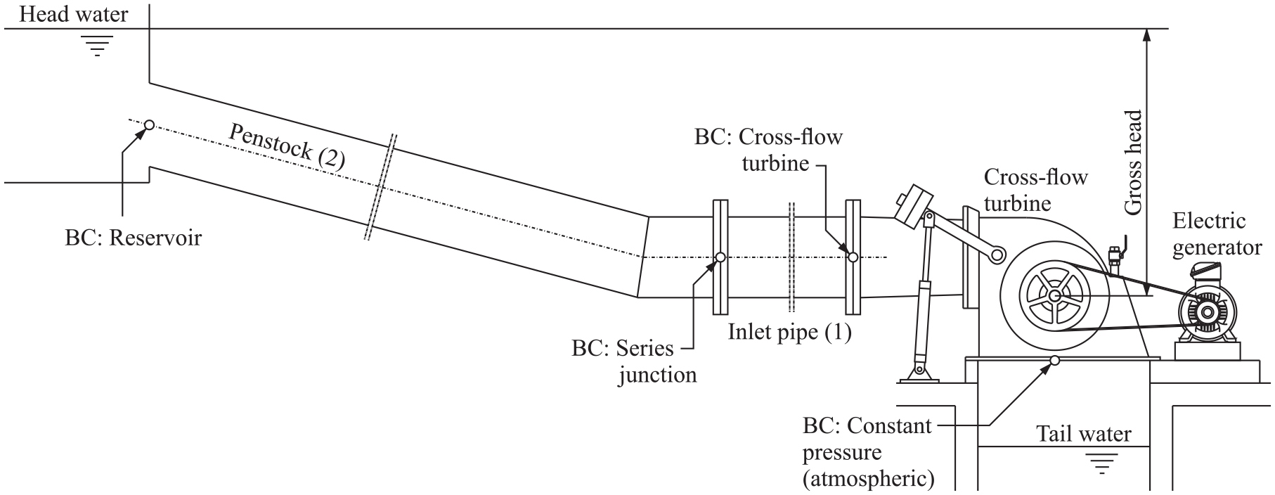
General sketch of a hydropower plant with cross-flow turbine.

The presented mathematical model of the transient-state operation of a hydropower plant with a cross-flow turbine was solved using software developed by the authors. The computational procedure applied for solving the unsteady flow equations (22) and (23) using the method of characteristics has been described in detail by Chaudry²⁶ and Watters.²⁸ The boundary conditions representing pipe junction and reservoir are also defined in the same literature. The friction term in equation (23) was integrated using a first-order approximation. The Darcy-Weisbach friction coefficient f was assumed to be constant during unsteady flow. The involvement of higher-order approximations of the friction term or unsteady friction was considered redundant in this case since the major uncertainty of the mathematical model arise from the estimated performance characteristic of the turbine.

The boundary condition ‘cross-flow turbine’ has been evaluated using an iterative procedure similar to that proposed by Chaudry²⁶ for the Francis turbine. The method of estimating the moment of inertia of a generator is given in the same literature. The overall moment of inertia of the runner, couplings and speed increaser was estimated at 10% of the moment of inertia of the generator. Assessment of the cross-flow turbine performance characteristics is described in detail in the previous section.

Since the computational domain given in Figure 6 comprises two different pipes, the time and spatial steps of the numerical (i.e. characteristic) grid have to satisfy the equation

Δ t = \frac{Δ x_{i}}{a_{i}} = \frac{L_{i}}{a_{i} n_{i}}, i = 1 to N

(24)

where n_i is the integer equal to the number of sections into which ith pipe is divided, and N is the number of pipes in the system (N = 2). As the wave velocity a_i cannot be calculated precisely, minor adjustments in its value are acceptable to obtain an integer number of sections (Chaudry²⁶).

In the three case studies presented in the following section, the characteristic grid was defined by setting the spatial step Δx₁ of the shortest pipe in the system (inlet pipe) equal to the length of that pipe (refer to Table 1). This resulted in a time step Δt ranging from about 10 to 20 ms. The spatial step Δx₂ of the penstock was then calculated using equation (24) and it ranged from approximately 6 to 11 m. Minor time steps did not lead to any improvement in the results, which indicates that the numerical scheme is convergent and stable.

Table 1.

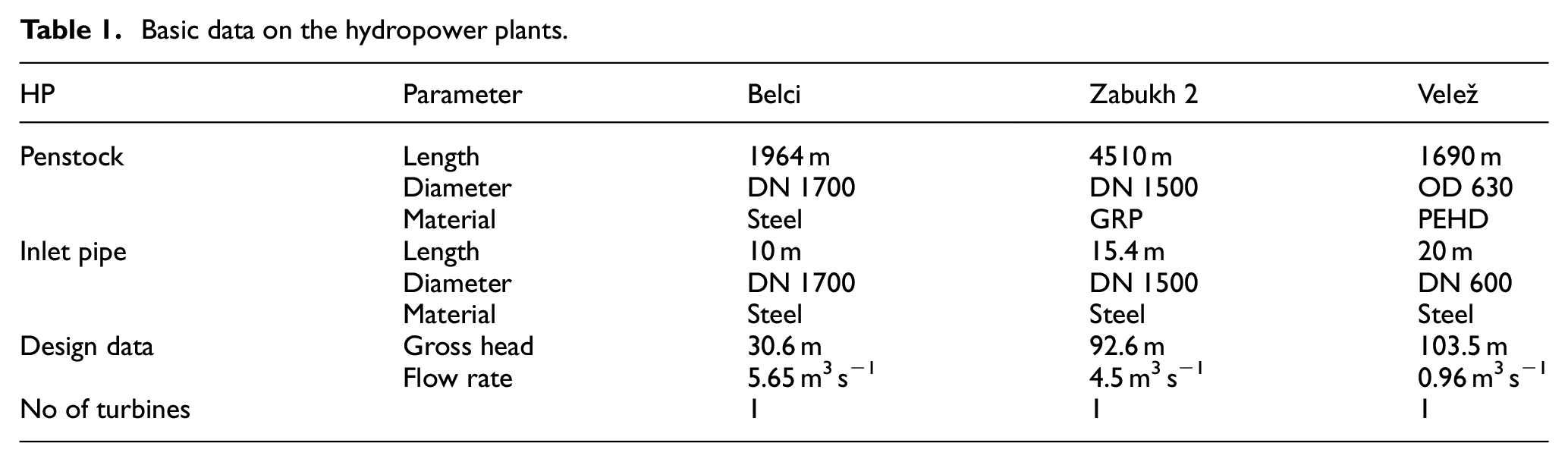
Basic data on the hydropower plants.

HP	Parameter	Belci	Zabukh 2	Velež
Penstock	Length	1964 m	4510 m	1690 m
	Diameter	DN 1700	DN 1500	OD 630
	Material	Steel	GRP	PEHD
Inlet pipe	Length	10 m	15.4 m	20 m
	Diameter	DN 1700	DN 1500	DN 600
	Material	Steel	Steel	Steel
Design data	Gross head	30.6 m	92.6 m	103.5 m
	Flow rate	5.65 m³ s⁻¹	4.5 m³ s⁻¹	0.96 m³ s⁻¹
No of turbines		1	1	1

Case studies

The presented mathematical model of transient-state operation of a hydropower plant with a cross-flow turbine is checked and validated by comparing the calculated flow and head (i.e. pressure) changes with the measured ones in three hydropower plants:

HP Belci at the river Jošanica in Serbia.

HP Zabukh 2 at the river Aghavno in Armenia.

HP Velež at the river Samakovska in Serbia.

Basic data on these hydropower plants are given in Table 1 while the data on the installed cross-flow turbines are given in Table 2. The values of specific speed, turbine speed, and runner diameter, calculated using the proposed regression equations (6) through (10) are also given in Table 2. The percentage differences between the calculated and actual values are given in parentheses. Bolded values in Table 2 refer to those used for the assessment of the turbine performance characteristics.

Table 2.

Basic data on the installed cross-flow turbines.

HP	Belci	Zabukh 2	Velež	Note
Rated head H_o (m)	31.6	85	88.4
Rated flow Q_o (m³ s⁻¹)	5.65	4.5	0.96
Rated power P_o (kW)	1471	3227	707 kW
Efficiency η_bep	0.84	0.86	0.85
Generator speed (min⁻¹)	1000	1000	600
Turbine speed n_o (min⁻¹)	169	298	600	Actual
	197 (+16.6%)	308 (+3.6%)	587 (–2.2%)	Equation (8)
	192 (+13.5%)	310 (+4.3%)	587 (–2.1%)	Equation (9) using assessed D
	194 (+15%)	309 (+3.9%)	600 (SYN)	Mean value of equations (8) and (9)
Runner diameter D (m)	1.25	1.25	0.6	Actual
	1.15 (–8%)	1.2 (–4%)	0.65 (+8.3%)	Equation (10), rounded
Specific speed n_s	86.5	65.6	58.9	Actual, equation (4)
	86.7 (+0.2%)	59.4 (–9.4%)	58.5 (–0.5%)	Equation (6)
	100.7 (+13.5%)	67.8 (+3.3%)	57.7 (–2%)	Equation (7)
	93.7 (+8.3%)	63.6 (–3%)	58.1 (–1.3%)	Mean value of equations (6) and (7)
Unit speed n_11o (min⁻¹)	37.6	40.4	38.3	Actual, equation (1)
	39.8 (+5.8%)	40.3 (–0.3%)	41.5 (+8.3%)	Equation (1) using assessed n, D
Unit flow Q_11o (m³ s⁻¹)	0.64	0.31	0.28	Actual, equation (2)
	0.76 (+18.1%)	0.34 (+8.5%)	0.24 (–14.8%)	Equation (2) using assessed D
Unit power P_11o (kW)	5.3	2.64	2.36	Actual –equation (3)
	6.26 (+18.1%)	2.86 (+8.5%)	2.01 (–14.8%)	Equation (3) using assessed D

Two independent calculations were performed in all three case studies: one using actual specific speeds, turbine speeds runner diameters and unit quantities, and the other based on the values calculated using regression equations (6) through (10).

All performed calculations refer to the transient operation of the system triggered by sudden load rejection. The steady-state refers to the fully opened guide vanes of the turbine. The closing law of the turbine guide vanes was assumed to be linear over the given closing time.

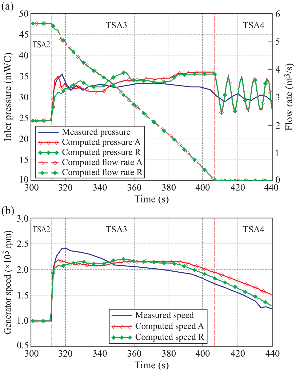
The data used for validation of the mathematical model refer to the in situ measurements of the pressure at the turbine inlet and the electric generator speed during the acceptance tests of the three selected hydropower plants. The data were obtained from the manufacturer of the cross-flow turbines. An example of the measurement results is given in Figure 7.

Figure 7.

Measurement results at the HP Zabukh 2 (courtesy of CINK Hydro – Energy k.s.).

The time intervals TSA2, TSA3, and TSA4 highlighted in Figure 6, indicate the following operating situations:

− TSA2 refers to the steady-state operation of the tested cross-flow turbine (n = const.).

− TSA3 is the time interval from the moment of intentionally induced load rejection up to the moment of closure of the turbine guide vanes (inlet pressure increases, the runner accelerates then starts to decelerate).

− TSA4 is the time interval after the closure of the guide vanes (inlet pressure oscillates, the runner slows down).

The available measured data and numerical results for all three hydropower plants were compared and discussed in the following subsections.

Hydropower Plant Belci

Figure 8(a) shows a comparison of the measured pressure at the inlet of the turbine in HP Belci and the calculated pressures at the same point. The time intervals TSA2, TSA3, and TSA4 have the same meaning as in Figure 7. The calculated flow rates at the turbine inlet are also given in Figure 8(a) although the measured flow was not available.

Figure 8.

HP Belci: (a) pressure at the turbine inlet and flow rate and (b) electric generator speed.

Figure 8(b) compares the measured and calculated rotational speeds of the electric generator connected to the observed cross-flow turbine.

The numerical results obtained using the actual specific speed, rated speed and runner diameter of the turbine are designated with ‘A’ in Figure 8, while the designation ‘R’ refers to the results based entirely on the regression equations (6) through (10).

By comparing the measured data and the numerical results given in Figure 8, the following conclusions can be drawn:

During the normal turbine operation (TSA2), the measured and calculated inlet pressures and electric generator speeds are identical, which is a good indicator that the transient-state hydraulic model of the system is properly defined.

From the moment of the load rejection up to the moment t ≈ 380 s, the calculated inlet pressure curves are close to the measured one, especially the pressure curve ‘A’. The discrepancy in the calculated pressures ‘A’ and ‘R’ is probably due to a significant difference between the actual and estimated unit flow Q_11o, unit power P_11o and especially the rated speed n_o (refer to Table 2). However, it should be noted that the measured and both calculated peak pressures in the same period are practically equal, although they are shifted in time. Such a result should be considered quite acceptable for an unsteady 1D model based on the estimated turbine performance characteristics.

Towards the end of the time interval TSA3 both calculated inlet pressure curves start to depart from the measured one, reaching a maximum difference of about +16% at the time of closure of the turbine guide vanes. A possible explanation for this discrepancy could be that the hydraulic cylinders that control the guide vanes opening were damped near the lower end of their stroke (e.g. to prevent a water hammer). In other words, the actual closing law of the turbine guide vanes is not linear, as is assumed in the model.

In the period after the guide vanes closure (TSA4), the calculated and both measured pressure changes show an oscillatory pattern that is typical of water hammer pressure oscillations caused by valve closure. However, the computed amplitudes of the inlet pressure oscillations are larger than the measured ones (by approximately 15%). Such a result supports the assumption that the hydraulic cylinders that control the guide vanes were damped to reduce the closing speed of the vanes at the end of their travel. The slower closing speed resulted in a milder deceleration of fluid flow, and hence milder pressure oscillations following the closure of the guide vanes.

Compared to the measurement, both calculated changes in the generator speed (and consequently the runner speed) show lower values after the load rejection and milder deceleration towards the end of the interval TSA3 and further during TSA4. This discrepancy could also be attributed to the nonlinear closing law of the guide vanes. Another cause may be that the estimated moments of inertia of the rotating mases (runner, speed increaser, couplings, generator) are larger than the actual ones. On the other hand, one of the most important parameters that must be controlled and limited is the maximum overspeed that the turbine (and generator) may attain in the event of a load rejection. In the analysed case, the calculated peak speeds differ from the measured one by only −9% (speed ‘R’) to −9.5% (speed ‘A’). This result shows that the proposed unsteady model can predict with sufficient accuracy the maximum overspeed during the emergency shutdown of the turbine triggered by load rejection. The maximum overspeed must be less than the turbine runaway speed, which is in the range of (1.9–2.3) × rated speed in the case of cross-flow turbines (IEC 62006²⁹).

Hydro Power Plant ZABUKH 2

Figure 9(a) shows a comparison of the measured and calculated pressures at the inlet of the cross-flow turbine in HP Zabukh 2. The calculated flow change is also given in Figure 9(a), although the flow rate was not measured on site. Figure 9(b) shows a comparison of the measured and calculated speeds of the electric generator. The highlighted time intervals as well as the designations ‘A’ and ‘R’ have the same meaning as in the previous case-study.

Figure 9.

HP Zabukh 2: (a) pressure at the turbine inlet and flow rate and (b) electric generator speed.

A brief analysis of the presented results leads to the following conclusions:

The calculated inlet pressures and generator speeds ‘A’ and ‘R’ are practically identical throughout the observed period. This indicates that the values of the specific speed, rated speed and runner diameter estimated using the proposed regression equations (6) through (10) are close to the actual ones (refer to Table 2).

The calculated inlet pressure curves closely follow the measured one in all three time intervals. The maximum difference between the calculated and measured pressure of −6% is at about 30 s after the moment of load rejection. This slight discrepancy could be due to the nonlinear stoke of the hydraulic cylinders that control the opening of the guide vanes of the actual cross-flow turbine. Nevertheless, what is the most important, the calculated and measured peak pressures are practically equal. Furthermore, unlike in the previous case study, the calculated and measured peak pressures occur at the same time, which indicates that the estimated performance characteristics of the turbine largely correspond to the real ones.

It is interesting to note that the measured amplitudes of pressure oscillations during TSA4 are now much closer to the calculated and larger than in the previous case study. It looks like the hydraulic cylinders of the guide vanes were not properly damped.

The calculated and measured electric generator speed change curves are practically the same almost until the end of the most important time interval TSA3. The calculated maximum speeds after the load rejection differ from the measured one by only −5% at t ≈ 295 s. The milder deceleration calculated at the end of the period TSA3 and during TSA4 could be attributed to the larger moments of inertia of the rotating mases estimated in the model and the nonlinear closing law of the actual turbine guide vanes.

Hydro Power Plant Velež

Figure 10(a) shows measured and calculated pressure changes at the inlet of the cross-flow turbine installed in HP Velež. Because the generator speed measurement was unavailable, Figure 10(b) only shows the calculated speed.

Figure 10.

HP Velež: (a) pressure at the turbine inlet and flow rate and (b) computed generator speed.

By analysing the results given in Figure 10, the following conclusions can be drawn :

The calculated pressures and speeds ‘A’ and ‘R’ are identical, which is mainly due to the equality of the estimated and actual speeds (synchronous), but also because the estimated values of specific speed and runner diameter are close to real ones (refer to Table 2).

The calculated and measured inlet pressures are almost identical except near the end of the period TSA3, where the maximum difference is about +5%.

In period TSA4 the calculated pressure oscillation amplitudes are larger that measured ones. The reasons for these slight deviations are probably the same as in the case of HP Belci.

Conclusion

Turbine performance characteristics (e.g. in the form of unit hill charts obtained from model tests) are essential data for analysing both the steady and transient operation of a hydropower plant. However, in the case of cross-flow turbines, the lack of their performance characteristics is a rule since the manufacturers generally do not provide them.

This paper presents a straightforward and rounded method for estimating the performance characteristics of an arbitrary cross-flow turbine even if only the net head and discharge of the turbine are known, for example, in the design stage of the hydropower plant. The assessed performance characteristics enable representation of the cross-flow turbine as the specific boundary condition within the mathematical model of the transient-state flow in hydropower plant systems.

Comparison of the numerical results and measurements performed on real hydropower plants with cross-flow turbines, showed very good agreement between the measured and calculated pressures at the turbine inlet as well as between the measured and calculated generator (i.e. turbine) speeds. Such a result shows that the developed mathematical model can be successfully used to predict the behaviour of a cross-flow turbine during transient regimes.

Further improvement of the presented mathematical model may be achieved by involving more than three known unit hill charts, which should result in a better assessment of the cross-flow turbine performance characteristics. A more precise estimation of the moments of inertia of the rotating mases (generator, runner, speed increaser, couplings) would also result in increased accuracy. Finally, the introduction of a more realistic guide vanes closing law would provide far better prediction of the cross-flow turbine behaviour during transient operation. This is clearly shown in the elaborated case studies in which the largest discrepancies between the calculated and measured inlet pressures and turbine speeds were due to the assumed linear guide vanes closing law. On the other hand, the presented mathematical model should serve as a tool for analysing different methods (including different guide vanes closing laws) for preventing or suppressing adverse outcomes of transients in hydropower plants with cross-flow turbines.

Footnotes

Appendix 1 Acknowledgements

The authors would like to thank the company CINK Hydro – Energy k.s. for providing the valuable test results used in this article.

Handling Editor: Chenhui Liang

Declaration of conflicting interests

The author(s) declared no potential conflicts of interest with respect to the research, authorship, and/or publication of this article.

Funding

The author(s) disclosed receipt of the following financial support for the research, authorship, and/or publication of this article: This work was supported by the Ministry of Education, Science and Technological Development, Republic of Serbia (contract number 451-03-68/2020-14200109).

ORCID iD

Slobodan Tašin

References

Riasi

Raisee

Nourbakhsh

. Simulation of transient flow in hydroelectric power plants using unsteady friction. J Mech Eng (Strojniški vestnik) 2010; 56: 377–384.

Garg

Kumar

. Experimental and numerical investigations of water hammer analysis in pipeline with two different materials and their combined configuration. Int J Press Vessel Piping 2020; 188: 104219.

Joukowski

. Mem Imperial Academy Soc of St. Petersburg 1898, 1900; 9(5); (in Russian, translated by Simin

. in Proc. Amer. Water Works Assoc. 1904; 24: 341–424).

Allievi

. Teoria del colpo d’ariete. Atti Collegio Ing Arch 1913; (English translation by Halmos

. The Theory of waterhammer. Trans Am Soc Mech Eng 1929).

IEC 60308:2005. Hydraulic turbines – testing of control systems.

Kodura

. An analysis of the impact of valve closure time on the course of water hammer. Arch Hydro Eng Environ Mech 2016; 63: 35–45.

Bergant

Mazij

Karadžić

. Design of water hammer control strategies in hydropower plants. Appl Eng Lett 2018; 3: 27–33.

Zhang

Cheng

Yang

, et al. Simulation of the load rejection transient process of a Francis turbine by using a 1-D-3-D coupling approach. J Hydrodyn 2014; 26: 715–724.

Wikipedia. Cross-flow turbine, https://en.wikipedia.org/wiki/Cross-flow_turbine (2021, accessed 10 September 2021).

10.

Adhikari

. Design improvement of cross-flow hydro turbine. Unpublished Doctoral Thesis, University of Calgary, Canada, 2016.

11.

AHEC-IITR. 1.2 and 2.1 general/ civil works – planning and layouts. Standard/manual/guideline with support from Ministry of New and Renewable Energy, Roorkee, 2013.

12.

Ossberger Hydro. Ossberger cross flow turbines, http://www.ossbergerhydro.com/cross-flow-turbines.html (2020, accessed 9 February 2021).

13.

Qian

Feng

, et al. Flow behaviors in a Kaplan turbine runner with different tip clearances. Adv Mech Eng 2021; 13: 1–15.

14.

Zhou

Shi

. Numerical and experimental investigation of the effect of baffles on flow instabilities in a Francis turbine draft tube under partial load conditions. Adv Mech Eng 2019; 11: 1–15.

15.

Mehr

Durali

Khakrand

, et al. A novel design and performance optimization methodology for hydraulic cross-flow turbines using successive numerical simulations. Renew Energy 2021; 169: 1402–1421.

16.

Jordan

. Study on reflected water hammer with special reference to Kaplan turbines. Serbia: University of Belgrade, Faculty of Mechanical Engineering, 1997 (in Serbian).

17.

Benišek

. Hydraulic turbines. Belgrade: Faculty of Mechanical Engineering, 1998, pp.195–238 (in Serbian).

18.

Kovalev

. Hydro turbines, design and construction. Leningrad: Mashinostroenie, 1971, pp.12–16 (in Russian).

19.

Kpordze

CSK

Warnick

. Experience curves for modern low-head hydroelectric turbines. Report No. PAP-451, Idaho Water Resources Research Institute, University of Idaho, Idaho, May 1983.

20.

Laboratory of Hydropower and Hydraulic Turbomachinery. Models of impellers, http://www.hydrolab.tu-sofia.bg/bg/documents/Models/Models.html (n.d., accessed 12 February 2021).

21.

Calov

. Research and development of cross-flow turbines. PhD Thesis, Technical University of Sofia, Bulgaria, 2015 (in Bulgarian).

22.

PT Entec Indonesia. MHP training Indonesia: Cross flow turbine. Presentation on theme: Cross flow turbine characteristic and layout, https://slideplayer.com/slide/13386557/ (n.d., accessed 5 February 2021).

23.

Iovănel

Bucur

Cervantes

. Study on the accuracy of RANS modelling of the turbulent flow developed uh Kaplan turbine operated at BEP. Part 1 – velocity field. J Appl Fluid Mech 2019; 12: 1449–1461.

24.

Durgin

Fay

. Some fluid flow characteristics of a cross flow type hydraulic turbine. In: Small hydro power machinery 1984. Presented at the winter annual meeting of the ASME, New Orleans, LA, USA, 9–14 December 1984, pp.77–83.

25.

Mockmore

Merryfield

. The Banki water turbine. Oregon State Engineering Experiment Station Bulletin Series 25. Corvallis: Oregon State College, 1949, pp.1–27.

26.

Chaudhry

. Applied hydraulic transients. 3rd ed. New York, Heidelberg, Dordrecht, London: Springer, 2014, p.159.

27.

Obradović

. Mathematical modelling of transients in hydropower plants. Belgrade: Energoprojekt-Energodata, 1981 (in Serbian).

28.

Watters

. Modern analysis and control of unsteady flow in pipelines. Collingwood: Ann Arbor Science Publishers, 1979, pp.47–82.

29.

IEC 62006:2010. Hydraulic machines – acceptance tests of small hydroelectricstallations.

Transient-state analysis of hydropower plants with cross-flow turbines