The effects of turbulent air streams and corrugated surfaces on the output of a wind turbine

Abstract

It is challenging to select the area that best fit the installation of wind turbines within complex and forestry terrains. This study aims to highlight the effects of corrugated surfaces on the characteristics of a turbulent wind flow, and on the performance of a wind turbine installed within this topography. It is hypothesized that a sinusoidal wave can be utilized to describe a corrugated surface. The physical stance was analytically modeled based on conservation principles of mass and mechanical energy. Model’s mathematical equation was then solved, by adopting finite difference method and MATLAB’s Bvp4c algorithm. The results show that wind and turbine related parameters are affected by the evolved atmospheric Boundary Layer (ABL) and differed according to the location within the boundary layer (BL) from the leading part to the edge, where BL’s retarding effects diminishes. The study also proves that velocity and turbine harvested power are inversely proportional to the corrugated surface’s amplitude, and to the wind’s turbulence ratio. On the other hand, it demonstrates a direct proportion between boundary layer thickness (BLT) and corrugated surfaces-related parameters. To the contrary of previous works, this study concentrated on capturing interaction effects between wind turbine, atmospheric inflow, and complex terrains.

Introduction

Both the roughness of the terrains surface and the turbulence of the airflow are major factors that affect local winds within any wind turbines farm. At higher locations over the ground level the wind becomes less influenced by the obstructions associated with the earth’s surface. However, within lower layers of the atmosphere, the air wind speed is affected by the friction against the earth’s geometry. As a result, it is important to consider the surface topologies effect on the air flow characteristics and the turbines parameters whilst selecting the location to install the wind turbines, this is vital for better performance and higher efficiency of the wind turbine.

There are several studies relevant to the scope of this manuscript: studied experimentally the influence of hills with applied roughness elements on the flow field and derived a power estimate of a standard wind turbine. Hyvärinen and Segalini ¹ carried out experimental measurements to study wind turbines over complex terrains in the presence of the atmospheric boundary layer. Thrust and power coefficients for single and multiple turbines were measured when introducing sinusoidal hills and spires inducing an artificial atmospheric boundary layer. Their results show hills have a positive impact on the wind-turbine performance.

Tianet al. ² conducted an experimental study to investigate the performance of wind turbines sited over hilly terrain. The study investigated the underlying physics to optimize the design of the wind turbines in relation to complex terrains. Ultimately their aim was to improve overall power yield and durability. They found that hill blockages disturb the downstream, which affects both the mean velocity and turbulence intensity in the flow. This leads to reduced power output and increased fatigue loads acting on wind turbines in such locations.

Turbulence flow plays a crucial role in wind energy as it usually causes unsteadiness performance of a wind turbine. ³ Yaliet al. ⁴ studied the flow pattern, wind speed and turbulence intensity over aligned arrays buildings with flat roof, gabled roof, pyramidal roof, and pitch roof, respectively. The appropriate wind profile supported urban rough atmospheric boundary layer was applied within the flow condition and Realizable k-ε turbulence model was used within the simulations. The results show that the flat roofs are best suited for turbine installation and then pyramidal roof is the next best solution. Pitch and gabled roofs are the worst.

Al-Qallab and Duwairi ⁵ studied the fluctuating laminar air stream potential of producing wind energy in addition to investigate different operating parameters of wind turbines. They established a mathematical model and solved the accompanied equation using MATLAB. They found that the increase of corrugated surface amplitudes decreases velocities inside boundary layers and reduce power output compared to those obtained by Blasius or traditional Pet theory.

Liu and Stevens ⁶ adopted Eddy simulations with an immersed boundary method to study the performance of wind turbines and wind farms in hilly terrain. They found that steep hills have a significant impact on the turbine’s power production, and that turbines that are significantly taller than the hill benefit from the speed up of the flow over the hill. For shorter turbines, they found that power production strongly depends on the turbine location in relation to the hill it reaches, its maximum value on the hilltop while locations at the bottom of the hill are worse.

There is apparently a research gap in literature, and the lack is in the analytical analysis of the along-boundary layer responses of wind-related parameters of a turbulent air streams flow over complex, and their impact on the performance of a wind turbine installed over these areas.

This study aims to highlight the effects on how the corrugated surfaces affect both turbulent wind flow characteristics and the performance of a wind turbine over this topography. It also analytically examines the productivity of wind turbines installed within a corrugated surface when turbulent air stream flows over the topography, using the along-boundary layer velocity instead of the free stream velocity, which is considered a new contribution to the field.

Modeling and analysis

Most studies in this field are experimentally based and very few studies analytically examine the responses of wind-related parameters when a turbulent air streams flow over a corrugated surface. Moreover, neither the air-related parameters along the evolved boundary layers, nor the productivity of installed wind turbine installed over such topography were thoroughly taken into consideration in these studies.

Fully developed flow over wavy surfaces, whether it is laminar or turbulent, is certainly more complicated than the ones developed over flat surfaces as there are extra parameters to be factored for as well as other related flow phenomena like wake effect.

In this manuscript, a new mathematical model based on conservation principles of mass and mechanical energy in addition to wind turbine equations was built and analyzed using a numeric computing platform. Furthermore, this study investigates wind power output and hydraulic characteristics inside and at the edge boundary layer, this includes derivation of governing differential equations, writing them in a dimensionless form, and solving the resultant equation numerically using MATLAB.

Coordinate system

Considering Steady state wind load for short periods can incarnate steady state wind model. Furthermore, the involving of incompressible wind model is justifiable; this is due to small forces of wind compared to a ramjet or turbojet. ⁵ The corrugated surface is modeled by the following function: $\sigma \left(x\right)=a\sin \sin \left(\frac{2\pi x}{\lambda }\right)$ . The model’s coordinate system is shown in Figure 1.

Figure 1.

Coordinate system of the model.

Governing equations

Model’s equation

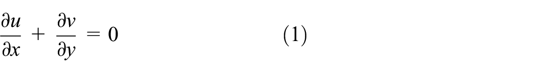
The Model’s governing equation are derived from:

• – Continuity equation ⁷ :

  $$\frac{\partial u}{\partial x}+\frac{\partial v}{\partial y}=0$$

  (1)

• – The x-momentum equation ⁷ :

  $$u\frac{\partial u}{\partial x}+v\frac{\partial u}{\partial y}=-\frac{1}{\rho }\frac{\partial p}{\partial x}+\frac{\mu }{\rho }*b(\frac{{\partial }^{2}u}{\partial x^2}+\frac{{\partial }^{2}u}{\partial y^2})$$

  (2)

• – The y-momentum equation ⁷ :

  $$u\frac{\partial v}{\partial x}+v\frac{\partial v}{\partial y}=-\frac{1}{\rho }\frac{\partial p}{\partial y}+\frac{\mu }{\rho }*b(\frac{{\partial }^{2}v}{\partial x^2}+\frac{{\partial }^{2}v}{\partial y^2})$$

  (3)

Where:

b = 1 + ε_m⁺, b is turbulence parameter, ε_m⁺ represents the dimensionless eddy viscosity, and defined by: ε_m⁺ =  $\frac{{\epsilon }_m}{v}$ , where $\nu$ is the kinematic viscosity, $\mu$ is the dynamic viscosity, p is the pressure inside the ABL, and $\rho$ is the air density.

The boundary conditions of interest are the no-slip boundary conditions at an impermeable ground, the viscosity, and the free stream boundary conditions without fluctuations at the boundary layer edge away from the surface.

The boundary conditions for no-slip conditions are given by:

$$\begin{array}{c}\multicolumn{1}{c}{@y=0,u(x,0)=0\mathrm{and}v(x,0)=0}\\ \multicolumn{1}{c}{\mathrm{When}\mathrm{y}\to \infty ,u(x,\infty )=u_{\infty }}\end{array}$$

The geometry of the adopted wave is shown in Figure 2.

Figure 2.

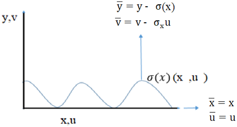
Representation of the corrugated surface function.

Introducing the corrugated surface related-parameters into equations (2) and (3) and simplifying yields:

$$\underset{¯}{u}\frac{\partial \underset{¯}{u}}{\partial \underset{¯}{x}}+\underset{¯}{v}\frac{\partial \underset{¯}{u}}{\partial \underset{¯}{y}}={\sigma }_x\frac{1}{\rho }\frac{\partial p}{\partial \underset{¯}{y}}+v*b(1+{{\sigma }_x}^2)\frac{{\partial }^2\underset{¯}{u}}{\partial {\underset{¯}{y}}^2}$$

(4)

$$\begin{array}{c}\multicolumn{1}{c}{{\sigma }_{x}u\frac{\partial \underset{¯}{u}}{\partial \underset{¯}{x}}+{{\sigma }_x}^{2}u\frac{\partial \underset{¯}{u}}{\partial \underset{¯}{y}}+{\sigma }_x\underset{¯}{v}\frac{\partial \underset{¯}{u}}{\partial \underset{¯}{y}}+{\sigma }_{\mathrm{xx}}{\underset{¯}{u}}^2}\\ \multicolumn{1}{c}{=-\frac{1}{\rho }\frac{\partial p}{\partial \underset{¯}{y}}-v*b*{\sigma }_x\frac{{\partial }^{2}u}{\partial y^2}(1+{{\sigma }_x}^2)}\end{array}$$

(5)

Combining equations (4) and (5), thus eliminating ( $\frac{\partial p}{\partial y^{}}$ ), leads to:

$$\underset{¯}{u}\frac{\partial \underset{¯}{u}}{\partial \underset{¯}{x}}+\underset{¯}{v}\frac{\partial \underset{¯}{u}}{\partial \underset{¯}{y}}=v*b(1+{{\sigma }_x}^2)\frac{{\partial }^2\underset{¯}{u}}{\partial {\underset{¯}{y}}^2}-\frac{{\sigma }_x{\sigma }_{\mathrm{xx}}}{1+{{\sigma }_x}^2}{\underset{¯}{u}}^2$$

(6)

The following transformations are introduced, and the well-known stream function (ψ) that relate velocity components (u, v) is also integrated to reduce the boundary layer equation from being with two dependent variables to an equation with a single dependent variable by implementing the following two equations ⁸ :

$$\eta =\sqrt{\frac{u_{\infty }}{\nu x}}y,\psi (x,y)=\sqrt{u_{\infty }\nu x}f(\eta )$$

After introducing the transformations, the Momentum’s equation is transformed into the following dimensional form:

$$f^{″\prime }+\frac{1}{2b(1+{{\sigma }_x}^2)}f{f}^{″}-x\frac{{\sigma }_x{\sigma }_{\mathrm{xx}}}{b{(1+{{\sigma }_x}^2)}^2}{f^{\prime }}^2=0$$

(7)

Equation (7) is dimensional, so it is converted to a non-dimensional form for generalization purposes. Therefore, the model’s final dimensionless mathematical equation becomes:

$${\mathit{f}}^{″\prime }+\frac{1}{2\mathbf{b}(1+{\mathbf{\sigma }}_{\mathbf{x}}^{*2})}\mathit{f}{\mathit{f}}^{″}-{\mathbf{x}}^{*}\frac{{\mathbf{\sigma }}_{\mathbf{x}}^{*}{\mathbf{\sigma }}_{\mathbf{xx}}^{*}}{\mathbf{b}{(1+{\mathbf{\sigma }}_{\mathbf{x}}^{*2})}^2}{{\mathit{f}}^{\prime }}^2=0$$

(8)

Where:

• – $x^{*}=\frac{x}{\lambda }$ , $a^{*}=\frac{a}{\lambda }$ , ${\sigma }^{\ast }\left(x\right)=\frac{{\sigma }^{}\left(x\right)}{\lambda }$ , ${\sigma }_x^{*}=\frac{{\sigma }_x}{\lambda }$ , ${\sigma }_{\mathrm{xx}}^{*}=\frac{{\sigma }_{\mathrm{xx}}}{\lambda }$ ; The dimensionless versions of $x,a,\sigma \left(x\right),{\sigma }_x\mathrm{and}{\sigma }_{\mathrm{xx}}$ , respectively.

• – The boundary conditions associated with this new equation are:

  $$f\left(0\right)=0,f^{\prime }\left(0\right)=0,f^{\prime }\left(\infty \right)=1$$

Boundary layer thickness (BLT)

BLT was calculated in this work using an algorithm that starts with dictating the location of the BL edge within ABL and ends with estimating BLT using the following equation:

$$y=\frac{\eta x}{\sqrt{R{e}_x}}$$

Where, y represents BLT if and only if $\eta$ equals to the value corresponds to $f^{\prime }$  ≥ 0.99 ×  $u_{\infty },$ that is starting from the edge of the BL.

Power calculations

Boundary layer based-power (corrugated surface power (P_corrugated))

In this study, the wind power extracted by the rotor blades of a wind turbine that takes into account BL effects due to the on-way corrugated surfaces is referred to as P_corrugated.

Starting from the general equation of power extracted by the rotor blades of a wind turbine ⁹ :

$$\mathrm{dP}\left(u(0,r)\right)=\frac{1}{2}\rho u^3(0,r)\mathrm{Cp}\mathrm{dA}$$

$$\mathrm{P}\left(\mathrm{u}(0,\mathrm{r})\right)=\underset{\mathrm{A}}{\overset{}{\int }}\frac{1}{2}\mathrm{\rho }{\mathrm{u}}^3\mathrm{Cp}\mathrm{dA}$$

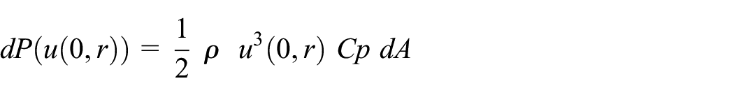
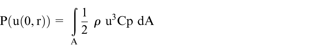
From this equation, it is clear that the potential power is calculated by considering the integration over the turbine’s blades (over the blade’s length (r)). It is also clear that the cubic of velocities across the turbine’s blades is integrated over the differential area (dA).

Thus:

$$P_{\mathrm{corrugated}}=\pi \rho \mathrm{Cp}{u}_{\infty }^3\underset{\eta 1}{\overset{\eta 2}{\int }}f{\prime }^3\left(\eta \right)(\frac{\eta 2*x^2}{R{e}_x}-\frac{H{b}_h*x}{\sqrt{R{e}_x}})d\eta$$

(9)

Free stream based-power (pet power (P_pet))

The wind power extracted by the rotor blades of a wind turbine term calculated by utilizing the free-stream velocity outside BL is referred to, in this study, as Pet power. It is the turbine’s rotor harvested power based on the free-stream without involving BL effects, thus the friction effect. The equation is ⁹ :

$$P_{\mathrm{pet}}=0.5*\rho *A_{\mathrm{swept}}*u_{\infty }^3*\mathrm{Cp}$$

(10)

The ratio P_corrugated to $P_{\mathrm{pet}}$ is computed and graphed for the sake of comparison.

Tip-speed-ratio (TSR)

TSR is one of the important parameters that must be included in any research conducted in the wind energy field. TSR is linked to efficiency and is calculated based on turbine’s radius (r), turbine rotational speed (ω) of the turbine and the average wind velocity across the turbine’s blades according to the equation ¹⁰ :

$$\mathrm{TSR}=\frac{(\omega *r)}{u_{\mathrm{avg}}}$$

Where ( $u_{\mathrm{avg}}$ ) is the average velocity across turbine blades that is calculated according to the equation:

$$u_{\mathrm{avg}}=\frac{\pi u_{\infty }\rho \mathrm{Cp}}{A_{\mathrm{swept}}}\underset{\eta 1}{\overset{\eta 2}{\int }}{f}^{\prime }\left(\eta \right)(\frac{\eta 2*x^2}{R{e}_x}-\frac{H{b}_h*x}{\sqrt{R{e}_x}})d\eta$$

(11)

It is essential when designing wind turbines to match the rotational speed of the rotor to the wind velocity so that an optimal rotor’s power efficiency can be achieved.

Numerical analysis

In this study, a MATLAB built-in code, named bvp4c has been adopted to numerically solve the final simplified nonlinear equation (8) derived above. Bvp4c is a built-in MATLAB solver whose target is to make solving a typical Boundary value problems (BVP) as simple as possible and Bvp4c solver executes a collocation strategy for the arrangement of BVPs. The solver determines the solution of a numerical expression by solving a global system of constraint conditions initiated by boundary conditions, and collocation conditions introduced on all sub-regions. The solver then calculates the error of the digital solution in each sub-period. If the solution does not meet tolerance condition, the analyzer adjusts the network and repeats the process, see Figure 3. ¹¹

Figure 3.

Flow chart of solving model’s equation numerically using the MATLAB program.

The expected numerical results for equation (8), at the given boundary conditions, will be:

• – Dimensionless stream function ƒ(η)

• – Dimensionless velocity profiles ƒ′(η)

• – Dimensionless shear stress function $f^{″}$ (η)

And the numerical analysis is accomplished as follows:

First, equation (8) is rewritten as a System of First-Order ODEs. The fundamental idea is to present new variables, one for each variable within the original problem, in addition to one for each of its derivatives up to one less than the highest derivative.

Let that be:

$$f\left(1\right)=ff\left(2\right)=f\prime f\left(3\right)=f\prime \prime$$

Accordingly, the final model’s equation has been coded to a system of first order equations as follows:

$$\begin{array}{c}f\left(2\right)=f\prime =0\hfill \\ f\left(3\right)=f\prime \prime =0\hfill \\ f^{″\prime }=x^{*}\frac{{{\sigma }_x}^{*}{{\sigma }_{\mathrm{xx}}}^{*}}{b{(1+{{{\sigma }_x}^{*}}^2)}^2}{f}^2\left(2\right)-\frac{1}{2b(1+{{{\sigma }_x}^{*}}^2)}f\left(1\right)f\left(3\right)\hfill \end{array}$$

The coded boundary condition related to the last equation can be written as:

$$f0\left(1\right)=0,f0\left(2\right)=0\mathrm{and}f\inf \left(2\right)=1$$

The equation and boundary conditions may be written in MATLAB as follows:

function dfdeta = fsode(~,f)

dfdeta = [ f(2)

           f(3)

(-.5/b*(1+z^2))*f(1)*f(3)+(q*z*z1/b*(1+z^2)^2)*f(2)^2];

end

function res = fsbc(f0,finf)

res = [f0(1)

  f0(2)

  finf(2) − 1];

knowing that (fsode) is a function that represents the equation as a system of first-order equations, and the boundary conditions described by (fsbc) function, where these functions must return column vectors to solve this problem with bvp4c solver.

Then initial guess of the solution is formed, the guess is provided to bvp4c in the form of a structure, which requires to contain two fields; (η) and ( $f$ ). A guess for a mesh that detects the behavior of the solution is provided as the vector solinit(η), While a guess for the solution at these mesh points is provided as the array solinit( $f$ ), with each column solinit( $f$ (:, i)) approximating the solution at the point solinit(η(i)).

Even though it is not difficult to form a guess structure, a helper function bvpinit can be used; it makes the structure when given the mesh and a guess for the solution in the form of a constant vector or the name of a function for evaluating the guess.

For the model’s equation an initial mesh of 100 points is created in the interval [0, $\infty$ ], where infinity is eta (η).

solinit=bvpinit(linspace(0,infinity,100),[0 0 0]);

At that point, the BVP solver employs the three inputs: (fsode: is the equation, fsbc: is the boundary conditions, solinit: is the initial guess), to solve the equation.

The yield of bvp4c is a structure called here sol.

sol = bvpsolver(@fsode,@fsbc,solinit);

The mesh decided by the code is returned as sol.x and the numerical arrangement approximated at these mesh points is returned as sol.y. Then put the output in cell array.

The working principle of the code is shown in the following flowchart:

Results and discussion

Validation of results

It is clear from the above equations, that the dimensionless velocity function ( $f\prime$ ) is the corner stone for the analysis of all wind-related, as well as turbine performance parameters. Thus the validation has been accomplished for this function, as follows.

Blasius model for flat plate laminar boundary layer is given by ⁸ :

$$f^{″\prime }+\frac{1}{2}f{f}^{″}=0$$

- The associated boundary conditions are: f(η) = 0, f′(η) = 0 at η = 0

f′(η) = 1 at η = ∞

Selected results from Blasius solution of the above equation, under the above boundary conditions, are shown in Table 1.

Table 1.

Flat plate laminar boundary layer functions. ⁸

$\eta$	$f$	$f\prime$	$f″$
0	0	0	0.332
0.4	0.027	0.133	0.331
0.8	0.106	0.265	0.327
1.2	0.238	0.394	0.317
1.6	0.420	0.517	0.297
2	0.650	0.630	0.267
2.4	0.922	0.729	0.228
2.8	1.231	0.812	0.184
3.2	1.569	0.876	0.139
3.6	1.930	0.923	0.098
4	2.306	0.956	0.064
4.4	2.692	0.976	0.039
4.8	3.085	0.988	0.022
5.2	3.482	0.994	0.011
5.6	3.880	0.997	0.005
6	4.280	0.999	0.002
6.4	4.679	1.000	0.001
6.8	5.079	1.000	0.000

This study’s model has been utilized to find the different dimensionless functions (stream (f_model), velocity (f′_model), and shear (f″_model)) associated with a flat plate laminar boundary layer for the same similarity variable values, and the results are compared with Blasius ones shown in Table 1. The comparison shows a good agreement and consistency, as shown in Table 2.

Table 2.

Validation of the results.

$\eta$	$f$	$f_{\mathrm{model}}$	% Error	$f\prime$	$f{\prime }_{\mathrm{model}}$	% Error	$f″$	$f\prime {\prime }_{\mathrm{model}}$	% Error
0	0	0	–	0	0	–	0.332	0.332127	3.80E−02
0.4	0.027	0.026566	1.66E+00	0.133	0.132792	1.5E−01	0.331	0.331539	1.62E−01
0.8	0.106	0.106131	1.2E−01	0.265	0.264764	8.9E−02	0.327	0.327456	1.39E−01
1.2	0.238	0.237999	4.2E−04	0.394	0.393857	3.6E−02	0.317	0.316652	1.09E−01
1.6	0.420	0.420408	9.7E−02	0.517	0.516861	2.6E−02	0.297	0.296718	9.4E−02
2	0.650	0.650158	2.4E−02	0.630	0.62989	1.6E−02	0.267	0.266795	7.6E−02
2.4	0.922	0.922476	5.1E−02	0.729	0.729121	1.6E−02	0.228	0.228122	5.3E−02
2.8	1.231	1.23122	1.7E−02	0.812	0.811657	4.2E−02	0.184	0.184023	1.2E−02
3.2	1.569	1.569396	2.5E−02	0.876	0.876233	2.6E−02	0.139	0.139132	9.4E−02
3.6	1.930	1.929887	5.84E−03	0.923	0.923481	5.2E−02	0.098	0.098082	8.3E−02
4	2.306	2.306169	7.3E−03	0.956	0.955667	3.4E−02	0.064	0.064226	3.5E−01
4.4	2.692	2.692842	3.1E−02	0.976	0.976017	1.7E−03	0.039	0.038964	9.2E−02
4.8	3.085	3.08586	2.7E−02	0.988	0.987932	6.8E−03	0.022	0.021864	6.1E−01
5.2	3.482	3.482463	1.3E−02	0.994	0.994386	3.8E−02	0.011	0.011336	3.0E+00
5.6	3.880	3.880942	2.4E−02	0.997	0.997616	6.1E−02	0.005	0.005428	4.4E+00
6	4.280	4.280327	7.6E−02	0.999	0.99911	1.1E−02	0.002	0.0024	2.0E+01
6.4	4.679	4.680118	2.3E−02	1.000	0.999748	2.5E−02	0.001	0.00098	2E+00
6.8	5.079	5.080075	2.1E−02	1.000	1.000	0	0.000	0.000369	–

Discussion of the results

Wind-related parameters

Dimensionless wind’s velocity ( ${\mathit{f}}^{\prime }$ )

$f^{\prime }$ profiles are estimated with respect to the similarity variable η over different physically meaningful selective values of a*, b, and x^*. Figure 4 shows that $f^{\prime }$ in accordance to η for selective values of a*, at b = 50,000 and x* = 1. It is obvious that as a* is increased, $f^{\prime }$ is accordingly decreased. This is rational; since higher a* means higher hill followed by a same height valley on the way of wind directed to an observer sitting just after the valley’s end of the first sinusoidal wave (x* = 1), and sensing a flurry with b = 50,000. The velocity will be decreased as these on-way obstructions become higher and deeper. The figure also shows that the maximum velocity happens when a* = 0, which refers to a flat surface without any restriction to the coming wind. The figure also refers to an increase of $f^{\prime }$ in the direction of BL growth. This increase ends at the edge of the BL, and at that position, wind velocity becomes equals to the free stream velocity ( $u_{\infty }$ ), therefore the fluid leaves the BL effect region. Furthermore, the figure tells us that under the predefined conditions, the velocity reaches BL edges only if the corrugated surface is transformed to a flat surface, while at any other a*, all wind velocities are located inside the BL and, thus, lesser than u_∞. Moreover, the figure also bids an abrupt decrease of $f^{\prime }$ as the obstruction becomes extremely high compared with its base length, as shown in the figure at a* = 25.

Figure 4.

$f^{\prime }$ versus η at different a*, b = 50,000, and x* = 1 hold unchanged.

The effect of changing b, holding a*, x* unchanged, is also analyzed. This can be conceived in the same manner as for a* = 1 explained above, where $f^{\prime }\mathrm{is}$ increased as $\eta$ is increased, but decreased with the increase in b from 10,000 to50,000. The analysis is performed under selective values of Turbulence parameter (b), see Figure 5.

Figure 5.

$f^{\prime }$ versus η at different b, a* = 1, and x* = 1 hold unchanged.

Figure 6 presents $f^{\prime }$ at different representative locations within the corrugated surface’s wave, such as; just before the start of the wave (i.e. the beginning of the hill), middle of the wave (i.e. at the normal earth level after ending the hill and before starting the valley), and at end of the wave (i.e. the end of the valley). These locations are represented by: x* = 0, 0.5, and 1, respectively. Other adopted locations are at the exact top of the hill (x* = 0.25) and the exact bottom of the valley (x* = 0.75). The later locations are referred to as sharply ended locations as it is incurred to an abrupt change from geometry increase to geometry decrease (x* = 0.25), or from geometry decrease to geometry increase (x* = 0.75). It is found that prominent values of $f^{\prime }$ happens at these locations, so they are representative. The analysis is conducted through adopting one of these location at a time, holding turbulence ratio (b) at 50,000, and hills/valley’s dimensionless height (a*) at 1.

Figure 6.

$f^{\prime }$ versus η at different x*, a* = 1, and b = 50,000 hold unchanged.

A thorough analysis of the figures, shows us that at the start/end locations along the wave, the curves of $f^{\prime }$ are congruous; that is $f^{\prime }$ values versus eta are the same. This is also the case at the sharply ended locations. That is vindicated mathematically because of the harmonic nature of the adopted sinusoidal waveform. However, at the above geometry locations, flurry has the same hydraulic characteristic. At sharply ended locations, $f^{\prime }$ has higher values than its analogs ones at start/end location, and this is easily understood as sharply ended locations lies on the highest/lowest points within the surface, this indicates the highest velocity among all wave’s locations. $f^{\prime }$ is affected by BL edge and employ a free stream velocity after this edge.

Boundary layer thickness (BLT)

BLT is analyzed against Reynold’s Number (Re) for the above different selective a*, b, and x* values, one at a time. Figure 7 shows the relationship between BLT and Re over the adopted values of a*. The figure marks that as Re is increased, BLT is decreased for all a* values. The physics behind that is attributed to the fact that fluids viscous force is getting smaller as Re is increased, holding inertia force unchanged. When fluid’s viscous force gets smaller, the fluids retarding effect accordingly gets smaller and the fluid easily gets toward BL edge and the free stream conditions. This behavior is obvious at flat surfaces (a* = 0). The figure also shows that all curves eventually go toward flatness as Re continues to increase, which in turn means that BLT decrease is ended, and BLT becomes constant and unresponsive to Re increase. On the other hand, as a* is increased, BLT is significantly increased. As elaborated on above, getting the obstruction amplitude bigger, leads the velocity values accordingly to get smaller. That establishes a bigger gap between the velocity inside BL and that at the free stream condition. Therefore, BLT gets bigger as a* is increased.

Figure 7.

BLT versus Re at different a*, b = 50,000, and x* = 1 hold unchanged.

Concerning the effect of turbulence on BLT, Figure 8 shows the relationship between BLT and Re at different b values. The figure indicates that as b is increased, BLT is significantly increased; this is assigned to the decrease of air flow velocity due to fluid layers disturbance, resulting from accumulated effects of Newton’s as well as Reynold’s stresses.

Figure 8.

BLT versus Re at different b, a* = 1, and x* = 1 hold unchanged.

The effect of variation x* on BLT is shown in Figure 9. It is noticeable that the response of BLT versus Re, under the different selective x* values, is repeated systematically for symmetrical x* values; that is when x* = 0, 0.5, 1, …, 20 from one side, and x* = 0.25, 0.75 from the other side. This is attributed to the sinusoidal-shaped model of the corrugated surface where the effects are repeated at the start/end as well as at sharply-ended positions. BLT is also changed periodically with x*. However, it is obviously larger at start/end positions (x* = 0, 0.5, 1, …, 20) in comparison to that at sharp ended positions (x* = 0.25, 0.75, …).

Figure 9.

BLT versus Re at different x*, a* = 1, and b = 50,000 hold unchanged.

Wind turbine performance parameters

One of the scopes of this work was to show that the velocity across wind turbine blades is changed as a result of boundary layer effect combined with the effect of the corrugated surface parameters (a* and x*) in addition to, the turbulence variable (b) effects. Average wind velocity across turbine blades should thus be employed when estimating all wind turbine’s related parameters such as TSR and the power, rather than adopting a constant free stream velocity, that imposes ignoring the retarding effects associated with the viscosity inside BL.

Tip speed ratio (TSR)

The analysis is achieved by employing a constant values of rotor rotational speed (ω) turbine blade length (r) throughout the analysis. Datasheet of Hitachi, HTW2.0-80 wind turbine is used (ω = 17.5 rpm, r = 40 m).

Figure 10 shows the relationship between TSR and Re at different a*. This figure illustrates that as Re is increased, TSR is decreased for all a* values. But the curves tend later toward flatness as Re continues increasing. These results are reasonable since increasing Re leads to an increase in the velocity across turbine blades, therefore average velocity, which will then tend to be constant at the edge of BL as previously elaborated, is also increased. This, in turn, leads to an inverse behavior of TSR with Re, followed by a flatness of the curves due to the same reason mentioned above. Also, as a* is increased, TSR is significantly increased. The reason behind that is the decrease in the velocity across turbine’s blades and this leads to a similar decrease in average velocity across the turbine blades and thus an increase in TSR and the final behavior of all curves will be the flatness.

Figure 10.

TSP versus Re at different a* (b = 50,000, x* = 1, $u_{\infty }$  = 5–20 m/s, Hb_h= 80 m, r = 40 m).

Figure 11 denotes that as turbine’s hub height (Hb_h) is increased, TSR is decreased for all a* values, but the curve tends later toward flatness as Hb_h continues increasing. This is due to the fact that the increase of Hb_h moves the average velocity across the turbine blades toward the inviscid region, which is obvious at flat surfaces (a* = 0), as previously dictated.

Figure 11.

TSP versus Hb_h at different a* (b = 50,000, x* = 1, $u_{\infty }$  = 10 m/s, r = 40 m).

Figure 12 presents the effect of Re on TSR at different b values. It is shown that TSR tends to converge around 4 as Re continues increasing at all b values. The reason behind that is imputed to the fact that increasing Re makes velocity range across turbine blades gets closer to/or out of the BL, therefore the average velocity across turbine blades reaches $u_{\infty }$ . On the other hand, the figure shows that as b is increased TSR also increased. This is again justified by decreasing average velocity across turbine as b is increased.

Figure 12.

TSP versus Re at different b (a* = 1, x* = 1, $u_{\infty }$  = 5–20 m/s, Hb_h= 80 m, r = 40 m).

The response of TSR with Hb_h at different b values is similar to that with Re but with the value of convergence located between 6 and 8. The reason behind that is as the turbine Hb_h is increased, the velocity range across the turbine become nearer or out relative to BL edge. Therefore, the value of average velocity tends consequently to be almost constant, as explained before, and thus having a constant TSR. As shown in Figure 13.

Figure 13.

TSP versus Hbh at different b (a* = 1, x* = 1, ${\mathit{u}}_{\infty }$  = 10 m/s, r = 40 m).

The effect of variation of x* is exposed in Figures 14 and 15. It is noticeable from these figures that the response of TSR versus Re and Hbh, is repeated systematically for symmetrical x* values. This is attributed to the sinusoidal-shaped model of the corrugated surface where the effects repeat at start/end as well as sharply-ended positions. TSR is also changed periodically with x*, and this is larger at the end positions (x* = 0, 0.5, 1, …, 20) in comparison to that at sharply-ended positions (x* = 0.25, 0.75, …), as shown in Figure 13.

Figure 14.

TSP versus Re at different x* (a* = 1, b = 50,000, $u_{\infty }$  = 5–20 m/s, Hb_h = 80 m, r = 40 m).

Figure 15.

TSP versus Hb_h aiot different x* (a* = 1, b = 50,000, $u_{\infty }$  = 10 m/s, r = 40 m).

The periodic response of the variation of TSR with Hb_h for different x* values is illustrated in Figure 15. It is shown that the variation of the turbine hub height has an inverse effect on TSR for all x* values. TSR is changed periodically with x*, and this change is larger at the start/end positions compared to that at sharply ended ones.

Power Results

Different results are presented in this section for the ratio of velocity range across turbine blades-based power to that based on the constant free stream velocity (pet power).

It is clear from Figures 16 to 18 that the power ratio is directly proportional to Re at the selected values of a*, b, and x* holding all other variables unchanged. This is imputed to the fact that increasing Re leads to a decrease in BLT due to the decrease in the viscous force that retards airflow in BL, as explained in details beforehand. Average velocity ranges across the turbine blades are accordingly moved toward the end of BL and may get out of it and approach $u_{\infty }$ . Consequently, wind turbine power ratio is increased and reached one in some cases. This is obvious when a* = 0, b = 1000, and x* = 0.25, 0.5, 1 shown in Figures 16 to 18 respectively.

Figure 16.

Power ratio (P_corrugated/P_pet) versus Re at different a* (x* = 1, b = 50,000, $u_{\infty }$  = 5–20 m/s, r = 40 m, Hb_h = 80 m).

Figure 17.

Power ratio (P_corrugated/P_pet) versus Re at different b (x* = 1, a* = 1, $u_{\infty }=$  5–20 m/s, r = 40 m, Hb_h = 80 m).

Figure 18.

Power ratio (P_corrugated/P_pet) versus Re at different x* (a* = 1, b = 50,000, $u_{\infty }$  = 5–20 m/s, r = 40 m, Hb_h= 80 m).

On the other hand, one can easily notice, from Figure 16, that the increase of a*, is accompanying by a decrease in power ratio. This decrease is slight at low obstruction altitudes; however, it becomes obvious if the obstruction height becomes very large compared with its base length. This is shown at a* = 25 curve in the same figure. The turbulence effect on the power ratio is also obvious; that is as b is increased, the power ratio is decreased, as shown in Figure 17. Such result is also accompanied by the decrease in the velocity across turbine blades because of fluid layer disturbance associated with the increase in b, as previously explained.

The variation of power ratio with x* is somehow different, where the variation of power ratio as Re changes follows the harmonic nature of the sinusoid-shaped model. Thus, the power ratio harmonically repeats itself as Re increases. The spot points adopted in this study are (x = 0, .25, 0.5, 0.75, 1, and 20). The results show that power ratio–Re curves are coincided both at x = 0, 0.5, 1, and 20 and at x = 0.25, 0.75. With lower power ratio values at x = 0, 0.5, 1, and 20, from one hand, and higher power ratio values at x = 0.25, 0.75, from the other hand, as shown in Figure 18.

The results also show that the turbine hub height plays a vital role in the power generated by the wind turbine located after the corrugated surface. It was found that increasing Hb_h, while keeping other independent variables unchanged, increases the power ratio in an even quantity depending on the values of a*, as presented in Figure 19. This result is attributed to the fact that as Hb_h, increases, the range of velocities passes through the turbine blades move toward or even exceeds BL edge, therefore, the average velocity across turbine blades increases, and thus the power ratio does. Furthermore, the figure exhibits that the increase in the obstruction height leads to a corresponding decreases power ratio.

Figure 19.

Power ratio (P_corrugated/P_pet) versus Hb_h at different a* (x* = 1, b = 50,000, $u_{\infty }$  = 10 m/s, r = 40 m).

Figure 20 bids the effect of Hb_h on the power ratio at different b values, keeping other variables unchanged. The response is a direct proportion with Hb_h, and inverse with b, studied under the condition of varying one variable at a time. The final destination of all curves is power ratio = 1.

Figure 20.

Power ratio (P_corrugated/P_pet) versus Hb_h at different b (x* = 1, a* = 1, $u_{\infty }$  = 10 m/s, r = 40 m).

Power ratio against Hb_h is also studied over a different model’s wavelength, keeping other variables unchanged. The results show a direct proportional. However, it also shows a periodic effect of power ratio for different values of x*. Similar to other x* results, the power ratio repeats itself either at sharply-ended locations of sinusoid waveform; x* = 0.25, 0.75, or at start/end locations; x* = 0.5, 1, …, 20, with the higher average velocities, and consequently power ratio, at sharply ended locations, compared to that at start/end ones, as shown in Figure 21.

Figure 21.

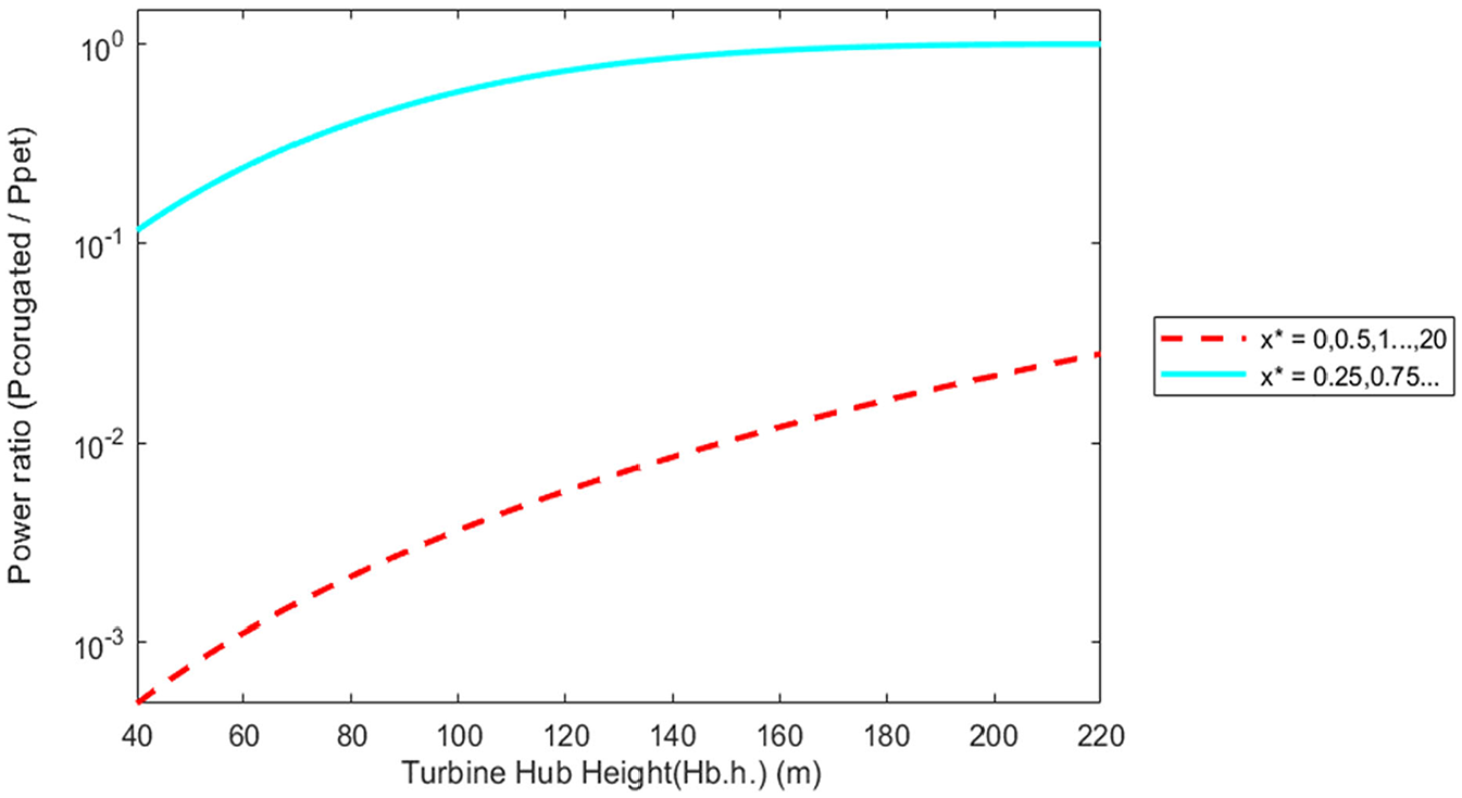
Power ratio (P_corrugated/P_pet) versus Hb_h at different x* (b = 50,000, a* = 1, $u_{\infty }$  = 10 m/s, r = 40 m).

Conclusion

The effects of turbulent air streams and corrugated surfaces on the output of a wind turbine have been investigated numerically. Different responses inside and at the edge of the evolved atmospheric boundary layer have also been studied in details. The study was accomplished analytically as follows: a mathematical model was established based on the conservation principles of mass and mechanical energy. The models mathematical equation was solved by utilizing MATLAB. The results are summarized as per below;

• – When an air stream with turbulent characteristics flows over a corrugated surface, its hydraulic characteristics such as velocity, turbulence ratio, and BLT are affected depending on the geometry of corrugated surface as well as fluid’s turbulence variable. The study has also proved that the performance of a wind turbine, installed within such topology, is also affected.

• – With elevation, the surface’s effects on the fluid flow is diminished rapidly and vanished completely outside the BL, where the flow velocity is returned to the freestream velocity, thus f′(η) becomes 1.

• – It was found that wind velocity and the turbine harvested power decreased as corrugated surface amplitude values are increased, and vice versa. On the other hand, BLT and fluid turbulence ratio have shown a direct proportional in this regard.

• – The way corrugated surfaces affect fluids parameters (such as wind velocity, BLT, and power) depends on the type of the waveform and the location within the waveform.

What is distinct in this work is shedding light on including not only free stream velocity as trend, but also along-BL velocity in all design, selection, and analysis processes of wind turbines.

The outputs of this study is hope to contribute to the endeavor of selecting the area that best fit the installation of wind turbine farms. In addition to the contribution toward wind turbines design purposes, and many other engineering applications such as evaluation of environment pollution.