Sage Journals: Discover world-class research

Abstract

This paper presents a study on the formability prediction, thickness variation, the influence of the gradient temperature, and prediction damage and failure behavior of aluminum sheets in a hydroforming vapor process through experimental and numerical investigations. A vapor hydroforming process that takes advantage of the coupling between thermal and mechanical loads applied to sheet metal is introduced. Uniaxial tensile tests and an optimization program developed in Matlab and based on the inverse method were conducted for identifying the coefficients of the Johnson-Cook law at room and at different temperatures. In parallel, a finite element model of the hydroforming vapor process was developed using ABAQUS/Explicit to reproduce the behavior of the aluminum sheet, where the behavior of the coupled thermo viscoelastic material and to the damage prediction of the plate being tested is analyzed using Johnson-Cook model. The results confirm the feasibility of the forming process. The variation of sheet thickness, the thinning mode of the tested sheet, and the effects of the hydroforming temperature are studied. A good agreement was achieved between experimental data and numerical results.

Keywords

Thin sheet experimental mechanics hydroforming 3D Johnson-cook numerical simulation

Introduction

In recent years, the hydroforming process of sheet or pipe has attracted the attention of many industries, especially in the automotive and aircraft industries.¹ Compared with traditional metal processing, sheet hydroforming (SHF) is particularly important in modern industrial manufacturing.^2,3 The SHF process has many advantages. For example, compared with deep drawing and extrusion processes, it can provide better product finishing. In addition, it saves costs and materials, reduces weight, improves quality, and improves accuracy. Several researchers have published studies on the forming process of pipes and plates with high-pressure fluids. Aissa et al.⁴ the influence of temperature on the formability of aluminum plates was studied experimentally using the steam hydroforming process. They showed that the electrical energy provided can increase the heating rate, but has no effect on the rupture pressure. In addition, the deformation in the thin plate reduces the stress flow and increases the plastic deformation under steam pressure. Modi and Kumar⁵ studied the numerical simulation of AA 5182 aluminum alloy sheet, and the influence of hydroforming process parameters (such as pressure path, blank clamping force, and peak pressure) on the deep drawing formability of the square cup, and verified through experimental data. Moreover, Jia et al.⁶ examined experimental and numerical the influence of internal pressure, friction coefficient, and loading path on tube forming quality in the hydroforming process. They concluded that the wall thickness near the corner is influenced by different loading paths and the degree of thinning is small in the transition area. In addition, Kang et al.⁷ investigated a numerical and experimental methodology to enhance hydroformability of complex tubular component with variable cross sections. They compared thickness variation between preformed hydroforming and non preformed hydroforming.

In the metal forming process, many researchers have been conducting SHF process research under hot temperature conditions and conducting thermomechanical analysis. Increasing the temperature of the forming process not only increases the formability, but also reduces the forming load and pressure. In order to obtain the highest formability, Acar et al.⁸ conducted a numerical study on the thermo-hydromechanical deep drawing (WHDD) process parameters of AA 5754-O, such as hydraulic pressure, blank bearing force load curve, and comparison with experimental method. They concluded that hydraulic pressure was found to be more effective on formability compared to the blank bearing force. In addition, the optimum temperature of the die and the blank holder is 300°C, and the optimum temperature of the punch is 25°C. The rapid increase in hydraulic pressure and the load curve of the blank support help to improve the formability. Mahabunphachai and Koç⁹ studied the effect of temperature on the microstructure of samples made of aluminum alloy AL5052 and AL6061, which have undergone biaxial and hydraulic expansion tests. The results show that the change of grain size is not significant due to the influence of high temperature and strain rate. Therefore, it can be concluded that the decrease in flow stress at high temperature is mainly due to thermally activated dislocation lines. In addition, the author further studied the influence of temperature and pressure on formability in a set of closed-mold warm forming experiments. The test results show that when a uniform temperature distribution of 300°C is applied, the linearly increasing pressure curve (up to the level of 20 MPa) has no significant effect on mold filling rate and part thinning. Janbakhsh et al.¹⁰ proposed an experimental study in which they used a hydraulic bulging process and a tensile test to evaluate the formability and determine the stress flow curve. Numerical results show the flow stress characteristics of biaxial load at higher strain levels compared with uniaxial load. It is also concluded that using Panknim’s protrusion radius and Kruglov’s thickness calculation method can obtain an accurate flow curve. Recently, Wang et al.^11,12 showed the improvement mechanism of the forming limit of the double-layer metal sheet through the hydraulic expansion test. They also studied finite element modeling (FEM) to study the influence of anti-wrinkle forming methods on the forming accuracy of 1060 aluminum sheet using paraffin wax. The experimental results show that increasing the molding pressure and the thickness of the paraffin layer can reduce the shape deviation of the molded parts. Cherouat et al.¹³ proposed a nonlinear anisotropic hardening method based on the elastoplastic constitutive equation. In addition, they studied the influence of water swelling conditions, internal pressure under various load curves, material ductility, and friction coefficient on the water formability of plates of different thicknesses. Johnson and Cook¹⁴ have developed a cumulative-damage fracture using a series cylinder-impact and biaxial tests data to determine fracture characteristics of OFHC copper, Armco iron, and 4340 steel. They concluded that the fracture depends on the hydrostatic pressure more than the strain rate and temperature.

In view of its importance in the industrial field, and aims to analyze, understand, optimize, and predict the influence of several parameters in the steam hydroforming process, this work aims to analyze the numerical simulation of coupled thermoviscoplastic material behavior. According to our experimental data in Aissa et al.^4,15 The Johnson-Cook plasticity model (JC) is used to predict the damage of aluminum plates. Two procedures were applied to identify the parameters of the JC model. The first is to determine the Johnson-Cook material and damage model through experiments. The second step includes the use of optimization algorithms developed under MATLAB and identification based on the inverse method. In addition, experimental data, numerical analysis are conducted to study the thinning mode and the influence of the hydroforming temperature on the used sheet.

Experimental investigation

Material and sample preparation

In this study, the sheet metal is AL1050 aluminum alloy, and the original blank is 1500 mm × 1000 mm × 0.6 mm. In order to prepare the sample for the expansion test, the piece was cut into disks with a diameter of 275 mm. The diameter of the steam pressure-bearing part of the blank is 160 mm. For the quasi-static test, three tensile tests were performed for each strain rate (2, 5, 10,15 mm/min) in order to obtain an average of the results. The drawing geometry of the sample along the rolling direction is shown in Figure 1.

Figure 1.

The sample geometry along the rolling direction (dimensions in mm) of Aluminum 1050.

Experimental test setup

The tensile test was carried out in the Mechanical Laboratory (ENSIT) of the Tunisian National Engineering College (see Figure 2). It is equipped with extensometer, high temperature furnace, and hot chamber. The quasi-static test is carried out at room temperature and different temperatures (20°C, 100°C, 200°C). They are carried out using a universal double-column test well machine with a load capacity of 100 kN and a strain rate ( $\overset{•}{\bar{ε}}$ ) of 2, 5, 10, 15 mm/min. The loading stopped when it dropped to 40% of the peak load.

Figure 2.

The tensile test setup.

Ultrasonic thickness measurement system

Figure 3 shows the experimental setup used to measure the thickness of the aluminum sheet. An ultrasonic measuring system is used to measure the varying thickness along the rolling direction and transverse direction of the experimental sample. Olympus 38DL PLUS ultrasonic thickness gauge is an advanced handheld instrument. 38DL PLUS is equipped with a thickness gauge and ultrasonic coupling gel. It is recommended to check rough surfaces to promote the transmission of sound energy between the thickness gauge and the sheet metal. The Olympus 38DL PLUS ultrasonic thickness measurement range used in this experiment is 0.08–635 mm, and the high resolution is 0.01 mm. Thickness measurement made at the sound speed of aluminum is equal to 5000 m/s.

Figure 3.

Ultrasonic thickness measurement system (Olympus 38DL plus ultrasonic thickness gauge).

Numerical modeling

Based on the experimental results of vapor hydroforming process of aluminum sheet metal shown in previous experimental work Aissa et al.^4,15 The numerical simulation of the metal forming process depends on the constitutive law used and its material parameter identification. In order to simulate the steam hydroforming process of aluminum sheet, the temperature dependence is considered in the current simulation.

Description of the numerical model

In this research, a three-dimensional thermoviscoplastic finite element model was established to simulate the steam hydroforming process to obtain the thermomechanical response of the metal sheet. Numerical calculations are carried out using commercial code ABAQUS/EXPLICIT software.¹⁶ All dimensions are the same as the actual settings shown in the experiment section. The Dies were modeled as an analytical rigid part, and the test plate is modeled as a deformable part. Increasing pressure is applied to the surface of the sheet.

Boundary conditions

According to the experimental results of the steam hydroforming process of aluminum sheet metal shown in the previous experimental work,^4,15 two steps were created. The first step is to firmly clamp the boundary of the initial blank around its boundary with the dies (see Figure 4). The second step is to apply the experimental laws of pressure and temperature. In the numerical simulation, the mixture of liquid water and water vapor is in equilibrium at the starting point. Research on the correlation between the pressure and temperature of saturated steam, show that there are empirical models involving thermodynamic variables which interpret the vaporization of water as a variable volume. These models⁴ can be written as follows:

\frac{P}{P_{0}} = K {[\frac{T - T_{0}}{100}]}^{n}

(1)

Figure 4.

Three-dimensional exploded view of numerical model used in the vapor hydroforming process.

Where P is the pressure, T (°C) is the steam temperature, P₀ is the reference pressure fixed at 8 bars, and $T_{0}$ (°C) is the initial temperature. K and n are the parameters of the model.

The sheet blank will gradually deform with the input of temperature and pressure, and gradually become smaller along the form of the table. Modeling the interaction between the dies and the sheet is one of the most important considerations necessary to correctly simulate the hydroforming process. The interaction characteristics between the contact area of the plate and the dies are defined by the Coulomb friction model, which is expressed as follows:

τ_{fric} = μ P

(2)

Where $τ_{fric}$ is the friction shear stress, $μ = 0.2$ is the friction coefficient, and P is the normal contact pressure.

Finite element mesh

The model consists of hexahedral elements with eight nodes, thermally coupled bricks, three linear displacements and temperatures, reduced integrals, and hourglass control. This element is represented as C3D8RT in the Abaqus software package, with unified strain and hourglass control. The finite element mesh consists of 15,276 nodes and 12,800 elements. Mesh allocation only involves deformable components. According to the grid sensitivity analysis, select the specification and size of the flake elements and the number of elements equal to 12,800. Figure 5(b) shows that the central part is meshed by using a fine grid, while the rest of the part we use a coarse grid as a whole. Considering the bending stiffness, the sheet is divided into three layers in the thickness direction. After several numerical simulations, the parameters (mesh, element type) of the finite element model are selected to evaluate their influence on the calculation time and obtain good results.

Figure 5.

Meshing configuration of the initial blank: (a) mesh detail of the die and (b) mesh detail of the sheet.

Material

Material of dies

Table 1 lists the mechanical properties of the upper and lower dies used.

Table 1.

Thermo-physical material parameters of the dies.

Material parameters of the dies	symbol	Values
Density (kg/m³)	ρ	7800
Poisson’s ratio	υ	0.3
Young’s modulus (MPa)	E	210,000
Heat conductivity (W/(m °C))	λ	48
Specific heat (J/(kg °C)]	Cp	473

Sheet material

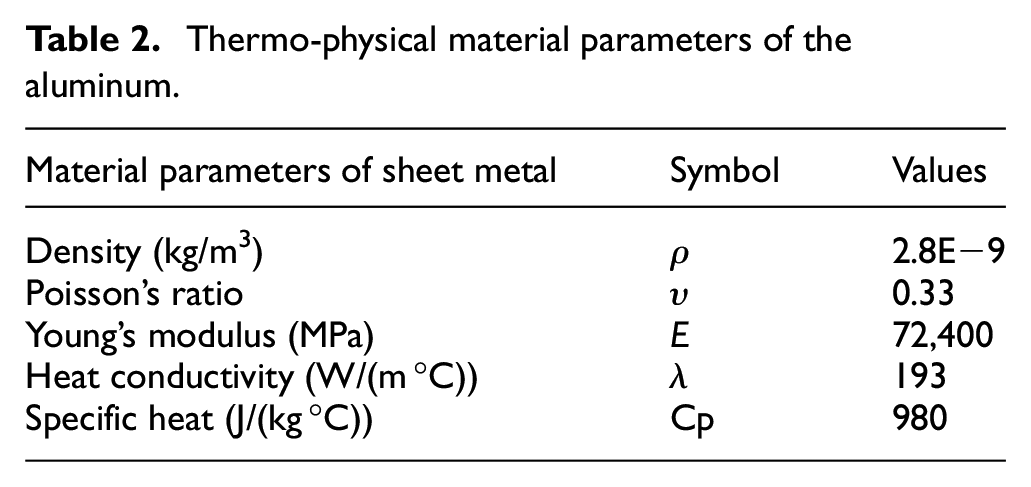
The sheet used for numerical simulation is 1050 aluminum alloy. The thermophysical material parameters used in the table are shown in Table 2:

Table 2.

Thermo-physical material parameters of the aluminum.

Material parameters of sheet metal	Symbol	Values
Density (kg/m³)	ρ	2.8E−9
Poisson’s ratio	υ	0.33
Young’s modulus (MPa)	E	72,400
Heat conductivity (W/(m °C))	λ	193
Specific heat (J/(kg °C))	Cp	980

Material constitutive models

Johnson-Cook material model (JC)

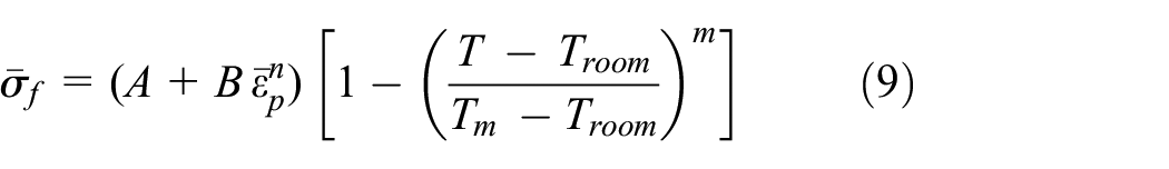
Determine the parameters of the Johnson-Cook (JC) constitutive model of aluminum 1050A for the numerical simulation of the steam hydroforming process. Therefore, this research proposes JC equivalent flow stress¹⁷ as an applied material model for sheets. It considers a simple form of the empirical relationship between stress and strain, strain rate, and temperature, as shown below¹⁸:

{\bar{σ}}_{f} = (A + B {\bar{ε}}_{p}^{n}) [1 + C Ln \frac{\overset{•}{\bar{ε}}}{\overset{•}{{\bar{ε}}_{0}}}] [1 - {(\frac{T - T_{room}}{T_{m} - T_{room}})}^{m}]

(3)

Where, A, B, n, C, and m are the constants of material, $\overset{•}{\bar{ε}}$ $\overset{\cdot}{\bar{ε}}$ is the strain rate which is normalized with a reference strain rate $\overset{•}{{\bar{ε}}_{0}}$ , $T_{room}$ represents the room temperature, and T_m is the melting temperature of the material equal to 911°K. The parameter n takes into account the strain hardening effect and the two coefficients m and C model respectively the thermal softening effect and the strain rate sensitivity.¹⁹

The yield criteria used in our finite element mode is the 3D Von Mises yield criteria given as:

σ_{Y} = \sqrt{\frac{{(σ_{1} - σ_{2})}^{2} + {(σ_{2} - σ_{3})}^{2} + {(σ_{3} - σ_{1})}^{2}}{2}}

(4)

Where $σ_{1}, σ_{2}, σ_{3}$ are the principal stresses from three-dimensional stress state.

Johnson-Cook damage model (JC)

The damage model proposed by Johnson-Cook was used together with his yield model. According to the classical damage law, the theoretical expression of this response in the finite element that represents the fracture or macroscopic crack caused by the material damage is defined as²⁰:

D = \sum \frac{Δ \bar{ε}}{{\bar{ε}}_{f}}

(5)

Where $Δ \bar{ε}$ is the increment of equivalent plastic strain during integration step, and ${\bar{ε}}_{f}$ is the equivalent strain value at fracture under current conditions.

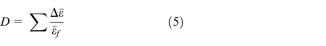
When the damage variable reaches its critical value (D = 1) in any element, rupture and damage will occur. The damaged element will be removed from the calculation. According to Johnson-Cook failure law, the general formula of fracture strain at critical failure can be written as²¹:

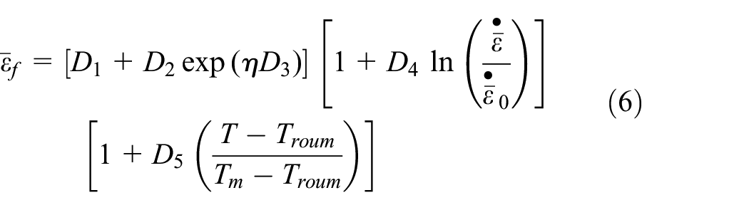
\begin{array}{l} {\bar{ε}}_{f} = [D_{1} + D_{2} \exp (η D_{3}] [1 + D_{4} \ln (\frac{\overset{•}{\bar{ε}}}{\overset{•}{{\bar{ε}}_{0}}})] \\ [1 + D_{5} (\frac{T - T_{r o u m}}{T_{m} - T_{r o u m}})] \end{array}

(6)

Where D₁ is the Initial failure strain, D₂ is the Exponential factor, D₃ is the triaxiality factor, D₄ is the strain rate factor, D₅ is the temperature factor, and η is the ratio of the hydrostatic pressure to the effective stress.

Identification of the constants of the Johnson-Cook model

Two recognition procedures were applied. The first is to identify the model in three steps, first strain hardening, then strain rate dependence, and finally temperature dependence using tensile testing. The second method is to use the optimization program developed based on the inverse method under Matlab, and identify all the parameters A, B, n, C, and m at the same time.

First method

The equation (3) shows the JC model is a function of von Mises tensile flow stress, in accordance with strain hardening, strain rate hardening, and thermal softening.

Where, the parameter A corresponds to the elastic limit, at 0.2% deformation, of the tensile curve as shown in Figure 6(a).

Figure 6.

The stress-strain curves in various strain rate and temperatures. (a) Tensile curve: σ = f(ε) of aluminum 1050 @ v = 2, 5, 10, and 15 mm/min. (b) Tensile curve: σ = f(ε) of aluminum 1050 @ v = 2 mm/min and different temperature.

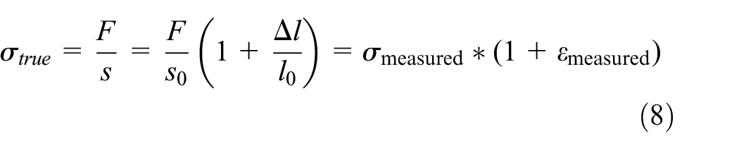
The hardening module B and the hardening coefficient n are determined from the plastic part of the tensile curve, transform the stress and the strain into true stress and true strain, and plot the logarithmic curve obtained in order to obtain an affine function as shown in Figure 7(a).

Figure 7.

The details determination of the parameters JC model. (a) Relationship between σ_true and ε_true under the reference conditions. (b) Relationship between ln(σ) and ln(strain rate) under the reference conditions. (c) Relationship between $\ln [1 - \frac{{\bar{σ}}_{f}}{(A + B {\bar{ε}}_{p}^{n})}]$ and $\ln [\frac{T - T_{room}}{T_{m} - T_{room}}]$ under the reference conditions.

The hardening module B is the value of the true stress when $ε_{plastic} = 1$ . While the hardening coefficient n is the slope of the curve plotted in the logarithmic tensile curve shown in Figure 7(a).

Were

ε_{true} = \ln (\frac{l}{l_{0}}) = \ln (\frac{s_{0}}{s}) = \ln (1 + ε_{measured})

(7)

and

σ_{true} = \frac{F}{s} = \frac{F}{s_{0}} (1 + \frac{Δ l}{l_{0}}) = σ_{measured} * (1 + ε_{measured})

(8)

The hardening module $B = e^{6, 087} = 440 MPa$ and the hardening coefficient n = 0.417.

The coefficient of dependence on the strain hardening rate C is determined from three strain-stress curves at room temperature but performed at different tensile displacement rates. It suffices to note the value of the stress for the same value of strain on these three curves, then to plot them in stress–logarithmic graph of the strain rate (see Figure 7(b)).

The hardening rate C is then the slope of the obtained curve. Therefore, for the strain rate sensitivity with tensile tests at several strain rates $C = 0.0076$ . The last coefficient to be determined is that of thermal softening m. Using the tests carried out in temperature (see Figure 7(c)).

When the deformation strain rate is $\overset{•}{\bar{ε}} = \overset{•}{{\bar{ε}}_{0}} = 2 s^{- 1}$ , equation (3) can be simplified as

{\bar{σ}}_{f} = (A + B {\bar{ε}}_{p}^{n}) [1 - {(\frac{T - T_{room}}{T_{m} - T_{room}})}^{m}]

(9)

Here, the influences of the strain strengthening effect are neglected. Equation (9) is rearranged into the following from:

\begin{matrix} 1 - \frac{{\bar{σ}}_{f}}{(A + B {\bar{ε}}_{p}^{n})} = {(\frac{T - T_{room}}{T_{m} - T_{room}})}^{m} \end{matrix}

(10)

Taking the natural logarithm on both sides of equation (10), the following equation can be obtained as:

\ln [1 - \frac{{\bar{σ}}_{f}}{(A + B {\bar{ε}}_{p}^{n})}] = m \ln [\frac{T - T_{room}}{T_{m} - T_{room}}]

(11)

Substituting the values of material constants, A, B, and n into equation (11) and fitting the data points using the first-order regression model. Value of m (1.005) is equal to the slope of the best line which passes through this scatter plot (see Figure 7(c)). For aluminum 1050, the thermal softening m = 1

The stress-strain curves in various strain rate and temperature shown in Figure 6(a) and (b).

Second method

In this case, the entire experimental database will be used. This method requires the order of magnitude of prior knowledge parameters to achieve the convergence of the algorithm. The best solution is the result of good agreement between the experimental response and the numerical response. The general recognition process is shown in the flowchart in Figure 8.

Figure 8.

Identification method by the inverse method.

The experimental data is expressed as a point in response to “load/displacement.” The relative difference between the experimental curve and the numerical curve is defined by formula (12):

ξ = \frac{1}{N} \sqrt{{\sum_{1}^{N} (\frac{F_{i \exp} (U_{\exp}) - F_{inum} (U_{\exp})}{F_{i \exp} (U_{\exp})})}^{2}}

(12)

Where $F_{\exp}$ is the experimental load, $F_{num}$ the numerical load, and $U_{\exp}$ the experimental displacement.

Use the following steps to determine the inverse identification method of Johnson-Cook behavior and damage model parameters:

✓Step 1: Identification of the J-C material model

•Step 1.1: Identification of the work hardening parameters A, B, and n with a cold tensile test.

•Step 1.2: Identification of the parameter C, using the obtained parameters A, B, and n in Step 1.1,

•Step 1.3: Identification of the parameter m, using the obtained parameters A, B, C, and n in Steps 1.1 and 1.2,

✓Step 2: Johnson-Cook damage model

•Step 2.1: Identification of the parameters $D_{1}$ , $D_{2}$ , and $D_{3}$ with a cold tensile test.

•Step 2.2: Identification of $D_{4}$ using the obtained parameters $D_{1}$ , $D_{2}$ , and $D_{3}$ in Step 2.1.

•Step 2.3: Identification of $D_{5}$ using the obtained parameters $D_{1}$ , $D_{2}$ , $D_{3}$ , and $D_{4}$ in Steps 2.1 and 2.2.

Tables 3 and 4 summarize the results of the research materials obtained by the two methods. The error is calculated for each parameter. For some parameters, this error reaches 20%. The parameter average values obtained by the two methods are used for numerical research.

Table 3.

Parameters of Johnson-Cook’s law for aluminum 1050 identified by two approaches.

	A (MPa)	B (MPa)	C	n	m	T (°C)
Approach 1: direct method	352	440	0.0076	0.42	1	20
Approach 2: reverse method	350	421	0.0063	0.35	1	20
Error %	0.57	4.51	20.6	20	0
Approach 1: direct method	245	198.94	0.0076	0.29	1	200

Table 4.

Johnson-Cook failure parameters for Aluminum 1050 by two approaches.

	$D_{1}$	$D_{2}$	$D_{3}$	$D_{4}$	$D_{5}$
Approach 1: direct method	0.13	0.13	−1.5	0.011	1
Approach 2: reverse method	0.14	0.14	−1.8	0.013	1
Error %	7.69	7.69	20	18.18	0

According to the Johnson-Cook fracture model, the fracture area is related to stress triaxiality and equivalent plastic strain. In addition, JCCRT is the Johnson-Cook damage initiation criterion, which is an evaluation value for evaluating damage based on the Johnson-Cook fracture criterion, which has a vital influence on material fracture. When JCCRT is greater than or equal to 1, it indicates that the material has broken. The mesh deletion technology used in the simulation will terminate the calculation after deleting a layer of elements.

Results and discussions

Formability prediction and thickness variation in experiment and finite element simulation of circular plate hydroforming

Theoretical background and hypotheses

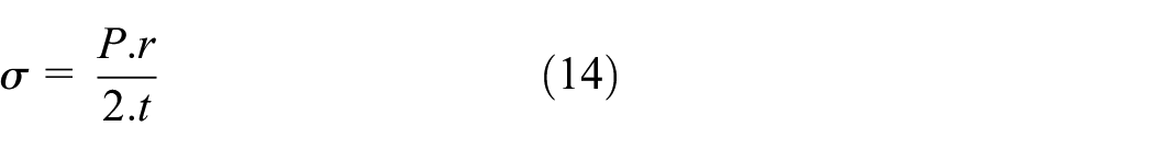
The purpose of the analysis method is to calculate the stress at the top of the dome in order to theoretically determine the flow curve and the thickness of the measured plate. The balance equation or Pascal equation is defined by

\frac{σ_{1}}{r_{θ}} + \frac{σ_{2}}{r_{φ}} = \frac{P}{t}

(13)

or $σ_{1}$ , $σ_{2}$ are the main stresses (assuming that the principal stress axes, (O, 1, 2, 3), and the orthotropy axes, (O, x, y, z), coincide), $r_{θ}$ and $r_{φ}$ are the radii of curvature respectively in the two main directions, P the hydraulic pressure and t the current thickness at the pole of the sheet (see Figure 9).

Figure 9.

Illustration of warm vapor bulge test: (a) initial and deformed configuration of the blank and (b) radii of curvature of the bulging sheet.

Finally, in cases of circular die and isotropic or anisotropic materials such that, the anisotropy coefficients at 0 and 90° are equal ( $r_{0} = r_{90}$ ), the principal stresses in the sheet plane are also equal ( $σ_{1} = σ_{2} = σ$ ), as well as the radii of curvature ( $r_{θ} = r_{φ} = r$ ), which simplifies equation (13) as follows:

σ = \frac{P . r}{2 . t}

(14)

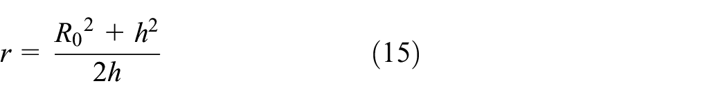
Assuming that the geometry of the deformed sheet is spherical, the radius of curvature r can be deduced from the height of the dome h over a radius $R_{0}$ according to the relation of the spherometer

r = \frac{{R_{0}}^{2} + h^{2}}{2 h}

(15)

The sheet plane ( $σ_{1} = σ_{2} = σ$ ). This assumption is adopted in the ISO 16,808:2014²² standard to enable the definition of the biaxial stress.

The sheet thickness t at the dome, is determined based on the knowledge of the initial value $t_{0}$ , and the transversal strain $ε_{3}$ , through the following equation:

t = t_{0} \exp (- ε_{3})

(16)

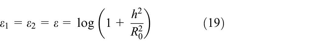
Based on the condition of volume constancy during the plastic deformation hence the principal strain $ε_{3}$ , is obtained from the principal strains in the sheet plane $ε_{1}$ and $ε_{2}$ at the dome:

ε_{3} = - (ε_{1} + ε_{2})

(17)

Since ε_{1} = ε_{2}

ε_{3} = - 2 ε_{1}

(18)

The strain gradient also affects the determination of the thickness strain. The mean meridian deformation for a given direction in an element is:

ε_{1} = ε_{2} = ε = \log (1 + \frac{h^{2}}{R_{0}^{2}})

(19)

From equations (12) and (15)

t = t_{0} {(1 + \frac{h^{2}}{R_{0}^{2}})}^{- 2}

(20)

σ = \frac{P {(R_{0}^{2} + h^{2})}^{3}}{4 t_{0} h R_{0}^{4}}

(21)

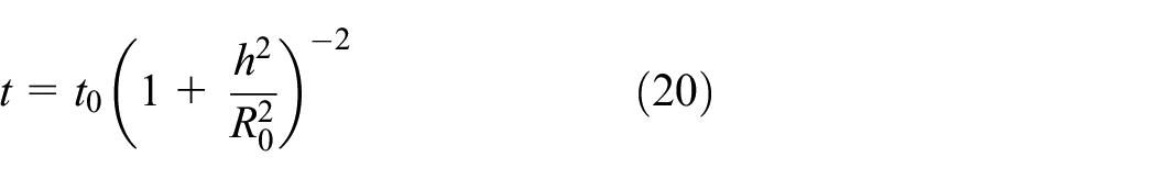
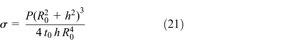
Figure 10(a) shows the experimental, analytical, and numerical results of the thickness change of the plate after the hydroforming test with steam along the radial path. The refinement is divided into two stages. The first one is located at the edge, which is characterized by its thickness slowly decreasing to 0.57 mm, and the temperature rising to about 125°C at a rate of about 0.0016 mm/°C can be considered quasi-static. The deformed state represents the heating of the water in the cavity and the rest of the equipment. The second stage is characterized in that the rapid growth rate of thinning can reach 0.012 mm/°C before rupture. The numerical method overestimates the degree of thinning of this material. The thickness distribution of the part predicted in the finite element simulation is also shown in Figure 10(b). The maximum thinning occurs at the dome of the cup, so when measured in the radial direction, the minimum thickness is at the edge about 0.329 mm. Although the thickness of the fractured sheet given by the analytical and experimental methods actually has the same value, about 0.40 mm, this represents a relative difference of about 21.2%. The decrease in thickness is related to a significant decrease in the maximum pressure recorded during the rupture.

Figure 10.

(a) Variation of the sheet thickness along a radial path and (b) Plot of the predicted thickness distribution from FEM analysis.

The concept forming limit curves

Figure 11 shows the conceptual forming limit curve, which is suitable for predicting the appearance of local necking during sheet hydroforming. In order to define the limit forming curve, a method similar to Hecker²³ is used. The image taken just before the rupture uses a very low flow rate, so there is not much distortion in this time interval, so it can be assumed that the image is very close to narrowing. Through the cross-section perpendicular to the rupture line, the maximum allowable deformation before rupture can be determined (Figure 11(a)). Then, the Bragard technique²⁴ is used to estimate the shrinkage deformation of the image taken after the fracture. Then draw this deformation as a defect deformation on the Hecker diagram (Figure 11(b)). The limit point represents the limit deformation of the aluminum plate 1050 in the plane of the aluminum plate 1050 through the steam hydroforming process for different loading paths. Figure 11(a) shows the ultimate deformation (no necking defect) corresponding to the successfully hydroformed part. Figure 11(b) shows failed parts with defects (necked or broken).

Figure 11.

The forming limit curve: (a) before failure and (b) after the failure.

Effect of the forming temperature on the hydroforming process:

Figure 12 shows the numerical and experimental results of two hydroforming tests performed when the sheet fails. The first test was carried out at room temperature (Figure 12(a)), while the second test was carried out with steam (Figure 12(b)). These tests were carried out on 1050A aluminum alloy sheets initially 0.6 mm thick.

Figure 12.

(a) Experimental and numerical tests at ambient temperature until the failure sheets. (b) Experimental and numerical tests with steam until the failure sheets.

The bulging pressure (P) and the dome height (h) values at the room temperature tests and the steam tests were used for the flow curve calculations (equations (19) and (21)). The flow curves in Figure 13 represent the material behavior of the aluminum alloy 1050A. The material model 1050 aluminum was also verified by the finite element analysis of the hydraulic expansion test, and its stress-strain curve was compared with the curve obtained from the experiment. These virtual and experimental hydraulic bulge tests were conducted at different temperatures. As shown in Figure 13, the numerical results and the experimental results are in good agreement no matter at room temperature or high temperature. The results obtained show a significant decrease in plastic flow stress. This decrease shows an alloy softening under the vaporization temperature effect. An increase in the limit deformations before bursting.

Figure 13.

Flow curves obtained from hydraulic bulge tests at room temperature test and steam test.

The expansion test is based on converting the thermal energy of steam generated in a closed enclosure into mechanical energy in the form of pressure applied to the inner wall of the sheet. During the experimental and numerical tests, the volume of steam and its expansion pressure increased simultaneously until it reached the stage of instability and sheet rupture, as shown in Figure 14.

Figure 14.

Combined effect of pressure and temperature on sheet volume.

For the steam hydroforming process, it is shown that the temperature conditions in the warm hydroforming process increase the forming limit of lightweight materials. Tracking the change in the thickness of the sheet during the steam expansion operation shows that the thickness steadily decreases slowly and then rapidly decays depending on the temperature of the steam generation. Therefore, an increase in temperature during the forming operation will cause an increase in the developing surface, which is equivalent to an increase in materials and a lighter weight of the finished part.

Figure 15 shows series results of seven values of an experimental and numerical steam hydroforming test. The sheet metal is AL1050 aluminum alloy, and the original blank is 1500 mm ×1000 mm ×0.6 mm. To prepare the samples for the expansion test, the sample was cut into disks with a diameter of 275 mm. The diameter of the steam pressure part of the blank is 160 mm. The bulge test of the sheet is stopped at a predefined temperature value (127°C, 136°C, 143°C, 155°C, 169°C, 175°C, 184°C).

Figure 15.

Steam hydroforming tests at different temperatures.

Figure 16 shows the thickness change at different temperatures. The graph shows the significant effect of temperature on the final cap thickness. In fact, the increase in sheet temperature will reduce the thinning of the hydroformed part, and therefore increase the surface area that is unfolded, resulting in an increase in material and a reduction in the weight of the resulting part. We also noticed from this figure that the thickness distribution corresponding to different temperatures can be approximated as a parabolic shape, which is characterized by a maximum located near the pole of the dome. These modes are represented by the equation (22), where parameter b is a constant, and a(T) is a function of the sheet heating temperature.

t = a (T) x^{2} + b

(22)

Figure 16.

Effect of hydroforming temperature on thickness distribution.

Fracture behavior of aluminum sheets under steam hydroforming process

Figure 17 shows the equivalent plastic strain distribution when the equivalent fracture initial stress is reached. According to the Johnson-Cook fracture criterion, visually judge whether there is a lack of mesh elements at the moment of cracking. The equivalent plastic strain around the crack area (Figure 17(a)) is equal to 0.438, in which the mesh elements are first deleted. Currently, this is the maximum value in the entire model at this moment. It means that the occurrence of initial fracture is related to equivalent plastic strain. In Figure 17(b), when the fracture starts, the maximum value of the equivalent stress does not exist near the fracture area where the mesh elements are deleted. Therefore, the maximum damage is not directly related to the value of the equivalent stress.

Figure 17.

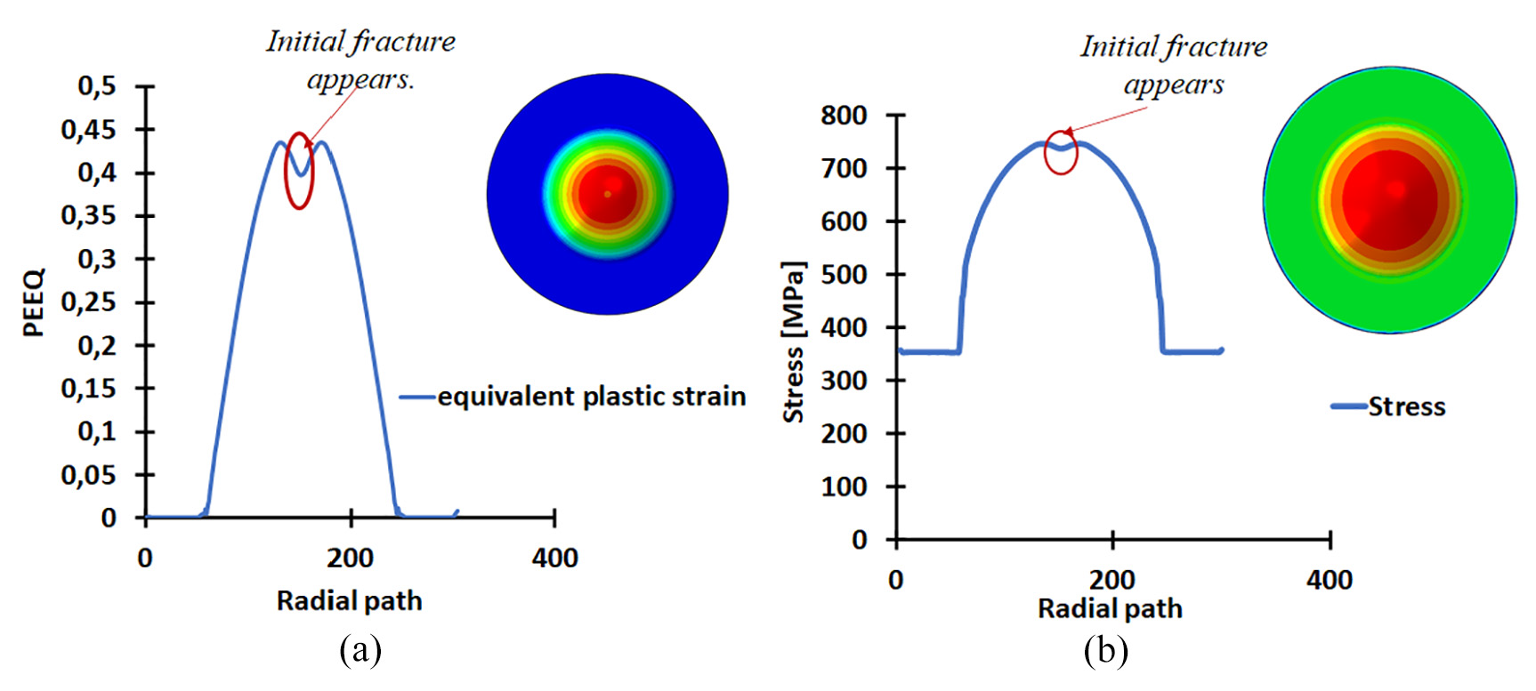
(a) Distribution of Equivalent Plastic Strain at the onset of fracture and (b) Distribution of the Von Mises stress at the onset of fracture.

Figure 18 shows the triaxial stress distribution and Johnson-Cook damage initiation criterion (JCCRT) when initial fracture occurs. The stress triaxiality in Figure 18(a) is equal to −1.943 near the fracture area. In the fracture area, the grid elements are deleted first and when they reach the minimum value. According to the equation (5), when ${\bar{ε}}_{f}$ equal to −1.5, the damage is inversely proportional to the triaxial stress, which is an important element in the Johnson-Cook fracture equation. The Johnson-Cook damage model is used to predict damage from numerical stress-strain data. It has a relatively acceptable damage prediction capability. When compared to the FLC method (Forming Limit Curve) where forming limit data is obtained experimentally, the JC damage can only provide approximate results. However, as shown in the results, the JC predicted damage results were quite satisfactory. In Figure 18(b), the JCCRT around the fracture area where the mesh elements are deleted shows that the evaluation value is consistent with the spinnability of the aluminum alloy 1050 during the vapor-phase hydrogenation forming process by the FE model.

Figure 18.

(a) Distribution of stress triaxiality at the onset of fracture and (b) Distribution of JCCRT at the onset of fracture.

It can be clearly seen from Figure 19 that the comparison of the fracture location between the finite element method and the experiment shows that the fracture location can be predicted according to the damage criterion Johnson Cook and the experimental process carried out on the 1050 aluminum plate. As shown in Figure 19, necking and fracture did indeed occur at the apex of the dome. This phenomenon is due to the influence of vapor pressure. The height of the dome predicted by numerical simulation is equal to 45 mm. This is also very consistent with the experimental data equal to 39 mm shown in Figure 20.

Figure 19.

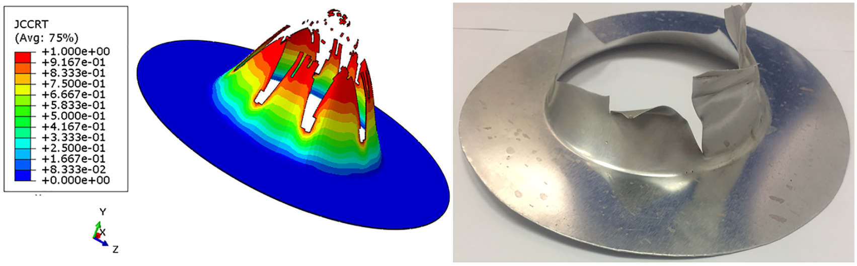
Crack distribution used for experiment and simulation at the end of steam hydroforming process.

Figure 20.

Experimental and numerical profiles of deformed sheet.

You may notice in Figures 19 and 20 that in the early stages of the process, the strain distribution in the central region is almost uniform. As the deformation progresses, the strain tends to be confined to a smaller area at the dome. Finally, this accumulation of strain leads to necking and fracture, as shown in Figure 19.

Figure 20 shows the significant difference in the pole displacement results obtained through experiments and numerical simulations during the steam hydroforming process. This can be justified by the stretching experienced by the sheet during the stage of sudden rupture. In fact, the pole is the area most prone to severe thinning, resulting in a significant decrease in the local stiffness of the thin plate. This creates other deformations, which can change the final appearance of the deformation.

Conclusions

This work puts forward the contradiction between the experimental data and the numerical study of the water vapor hydroforming test on the aluminum plate. Perform a hydroforming test until the aluminum sheet breaks. Two recognition procedures were applied. The first method is to use a tensile test at room temperature and different temperatures to determine the coefficients of the Johnson-Cook law. The second method of identification is to use an optimization program based on the inverse method developed under Matlab. The best solution achieved good agreement between experiment and numerical response.

The study on the thickness change of the measured board shows that there is a good agreement between the experimental, theoretical, and numerical results. Two sparse areas were identified. The first feature is that the changes are small. It is located at the edge and is affected by boundary conditions. The second area showed rapid thinning to reach the minimum thickness, which caused the sheet to crack.

In order to define the forming limit, determine the point that represents the ultimate deformation in the plane of the studied sheet. The results obtained show that the temperature conditions in the hot hydroforming process increase the sheet forming limit.

Applying a higher temperature gradient in the active sheet area can provide higher formability because the high temperature in the active area can increase the ductility of the sheet. In addition, the low temperature in the active sheet area increases the flow stress of the sheet to delay local thinning and failure.

The fracture behavior of aluminum sheet subjected to a hydroforming process with water vapor is studied. The distribution of equivalent plastic deformations in the tested sheet is studied and the maximum plastic deformation an indicator of the onset of fracture is determined.

The distribution of the triaxiality of the stresses and the Johnson-Cook damage initiation criterion (JCCRT) are studied respectively. The triaxiality of the stresses is calculated around the fracture zone where the mesh elements are removed first and reach the minimum value at that time.

The JCCRT is equal to unity around the fracture zone where the mesh elements are removed first. It demonstrates that the evaluated value conforms to the FE model for the spinnability of the sheet under study during the steam hydroforming process.

The results show that the finite element method can predict the maximum strain and stress and the location of the initial crack in the steam pressure hydroforming test.

Footnotes

Handling Editor: Chenhui Liang

Declaration of conflicting interests

The author(s) declared no potential conflicts of interest with respect to the research, authorship, and/or publication of this article.

Funding

The author(s) received no financial support for the research, authorship, and/or publication of this article.

ORCID iD

Mohamed Soula

References

Bell

Corney

Zuelli

, et al. A state of the art review of hydroforming technology: its applications, research areas, history and future in manufacturing. Int J Mater Forming 2020; 13: 789–828.

Lang

Wang

Kang

, et al. Hydroforming highlights: sheet hydroforming and tube hydroforming. J Mater Process Technol 2004; 151: 165–177.

Geiger

Merklein

Cojutti

Hydroforming of inhomogeneous sheet pairs with counterpressure. Prod Eng 2009; 3: 17–22.

Aissa

Mohamed

Tarek

Experimental study of steam hydroforming of aluminum sheet metal. Exp Tech 2017; 41: 525–533.

Modi

Kumar

DR.

Optimization of process parameters to enhance formability of AA 5182 alloy in deep drawing of square cups by hydroforming. J Mech Sci Technol 2019; 33: 5337–5346.

Jia

Luo

Analysis and experiment on tube hydroforming in a rectangular cross-sectional die. Adv Mech Eng 2017; 9: 1687814017694831.

Kang

Joo

, et al. Enhancing hydroformability of nonaxisymmetric part with variable cross section. Adv Mech Eng 2015; 7: 1687814015604547.

Acar

Türköz

Gedikli

, et al. Warm hydromechanical deep drawing of AA 5754-O and optimization of process parameters. J Eng Mater Technol 2017; 140: 011012.

Mahabunphachai

Koç

Investigations on forming of aluminum 5052 and 6061 sheet alloys at warm temperatures. Mater Des 2010; 31: 2422–2434.

10.

Janbakhsh

Djavanroodi

Riahi

Utilization of bulge and uniaxial tensile tests for determination of flow stress curves of selected anisotropic alloys. Proc IMechE, Part L: J Materials Design and Applications 2013; 227: 38–51.

11.

Wang

Yang

Bai

, et al. Evaluation of limit deformation behavior in hydro-bulging of the double-layer sheet metal using diffuse and localized instability theories. Int J Mech Sci 2019; 150: 145–153.

12.

Wang

Effects of wrinkling prevention forming method using paraffin on forming accuracy for 1060 aluminum sheet metal. Int J Mater Forming 2019; 12: 889–898.

13.

Cherouat

Ayadi

Mezghani

, et al. Experimental and finite element modelling of thin sheet hydroforming processes. Int J Mater Forming 2008; 1: 313–316.

14.

Johnson

Cook

WH.

Fracture characteristics of three metals subjected to various strains, strain rates, temperatures and pressures. Eng Fract Mech 1985; 21: 31–48.

15.

Aissa

Ali

Mahfoudh

Assessment of steam forming performance of aluminum sheet metal based on experimental studies. Int J Mater Forming 2020; 13: 639–647.

16.

Dassault Systèmes Simulia Corp. Abaqus 6.14 documentation. Providence, RI, USA: DSS, 2014.

17.

Wang

Lin

A comparative study on Arrhenius and Johnson–cook constitutive models for high-temperature deformation of Ti₂AlNb-based alloys. Metals 2019; 9: 123.

18.

Ijaz

Zain-ul-abdein

Saleem

, et al. Modified Johnson-cook plasticity model with damage evolution: application to turning simulation of 2xxx aluminium alloy. J Mech 2017; 33: 777–788.

19.

Murugesan

Jung

DW.

Johnson Cook material and failure model parameters estimation of AISI-1045 medium carbon steel for metal forming applications. Materials 2019; 12: 609.

20.

Ijaz

Zain-ul-abdein

Saleem

, et al. Numerical simulation of the effects of elastic anisotropy and grain size upon the machining of AA2024. Mach Sci Technol 2018; 22: 522–542.

21.

Banerjee

Dhar

Acharyya

, et al. Determination of Johnson cook material and failure model constants and numerical modelling of Charpy impact test of armour steel. Mater Sci Eng A 2015; 640: 200–209.

22.

Reis

Prates

Oliveira

, et al. Anisotropy and plastic flow in the circular bulge test. Int J Mech Sci 2017; 128–129: 70–93.

23.

Hecker

. A simple forming-limit curve technique and results on aluminum alloys. In: Proceedings of 7th biennial congress of the International Deep Drawing Research Group, Amsterdam, 1972.

24.

Bragard

Baret

Bonnarens

A simplified technique to determine FLD at the onset of necking. Rapport du Centre de Recherches Mettallurgiques, No. 33, 1972.

The behavior and forming performance of vapor hydroforming process of thin aluminum sheets: Numerical and experimental analysis

Abstract

Keywords

Introduction

Experimental investigation

Material and sample preparation

Experimental test setup

Ultrasonic thickness measurement system

Numerical modeling

Description of the numerical model

Boundary conditions

Finite element mesh

Material

Material of dies

Sheet material

Material constitutive models

Johnson-Cook material model (JC)

Johnson-Cook damage model (JC)

Identification of the constants of the Johnson-Cook model

First method

Second method

Results and discussions

Formability prediction and thickness variation in experiment and finite element simulation of circular plate hydroforming

Theoretical background and hypotheses

The concept forming limit curves

Effect of the forming temperature on the hydroforming process:

Fracture behavior of aluminum sheets under steam hydroforming process

Conclusions

Footnotes

Declaration of conflicting interests

Funding

ORCID iD

References