Sage Journals: Discover world-class research

Abstract

While calculating intercoder reliability (ICR) is straightforward for text-based data, such as for interview transcript excerpts, determining ICR for naturalistic observational video data is much more complex. To date, there have been few methods proposed in literature that are robust enough to handle complexities such as the occurrence of simultaneous event complexity and partial agreement by the raters. This is especially important with the emergence of high-resolution video data, which collects nearly continuous or continuous observational data in naturalistic settings. In this paper, we present three approaches to calculating ICR. First, we present the technical approach to clean and compare two coders’ results such that traditional metrics of ICR (e.g., Cohen’s κ, Krippendorff’s α, Scott’s Π) can be calculated, methods previously unarticulated in literature. However, these calculations are intensive, requiring significant data manipulation. As an alternative, this paper also proposes two novel methods to calculate ICR by algorithmically comparing visual representations of each coders’ results. To demonstrate efficacy of the approaches, we employ all three methods on data from two separate ongoing research contexts using observational data. We find that the visual methods perform as well as the traditional measures of ICR and offer significant reduction in the work required to calculate ICR, with an added advantage of allowing the researcher to set thresholds for acceptable agreement in lag time. These methods may transform the consideration of ICR in other studies across disciplines that employ observational data.

Keywords

methods in qualitative inquiry observational research mixed methods ethnography virtual environments

Introduction

In qualitative research, determining intercoder reliability (ICR), is one way to continually establish quality and reliability of analysis methods (Long & Johnson, 2000; Walther et al., 2013). The term intercoder reliability is synonymous with interrater reliability, two terms for the same concept of measuring agreement between two researchers, or raters, as they interpret the data through an established codebook. Agreement coefficients such as Cohen’s κ(Cohen, 1960), Scott’s Π (Scott, 1955), Krippendorff’s α (Krippendorff, 1970), Gwet’s AC (Gwet, 2008), and the G-Index (Holley, 1964, Brennan & Prediger, 1981) differ in their corrections for chance agreement in different situations, but without extensive manipulation, are limited to easily classifiable data with well-defined units of analysis and require exclusivity of codes such that only one code can describe each unit of data.

Extending methods for ICR and IRR calculation into naturalistic, ethnographic, or time-resolved (e.g., the capture of data as a function of time) observational research contexts is important. No longer limited to interview or textual analysis methods, qualitative methods now extend to analysis of video and surveillance data (e.g., Ko, 2011); eye-tracking data (e.g., Jacob, 1995; Zu et al., 2017), classroom observations (e.g., Alford et al., 2016; Tong et al., 2020), team performance observations (e.g., Waller & Kaplan, 2018, Klonek et al., 2019), or any other phenomena in which researchers seek to investigate patterns of events/behavior occurring over a duration of time. With advances in technology for data collection, many of these methods allow researchers to change from investigating a static definition of process (e.g., what behaviors occur in aggregate as a percentage of time) to a dynamic view of process by studying temporal dynamics of behavioral patterns using “high resolution” methods (those with high to near-continuous rates of data collection), including audio, video, digital data, and wearables.

While the calculation of intercoder reliability is acknowledged to be quantitative in that it requires numerical calculations, the calculation of inter- and intra-coder reliability is an essential part of qualitative research. Especially in increasingly complex research situations requiring observational data collection and subsequent interpretive analysis, qualitative researchers cannot ignore ICR metrics simply because the data are complex. Indeed, as we see in our review of the literature, many papers that employ naturalistic observation methods avoid ICR, code to agreement, or do not account for complexities inherent in coding such as partial agreement between researchers or the occurrence of simultaneous codes. However, as Erlingsson and Brysiewicz (2017) argued, if researchers do not measure intercoder reliability, their data are no more reliable than the subjective impressions of a single rater. As an effort toward developing streamlined methods to conquer the intricacies of reporting intercoder reliability, even for complex qualitative data, this paper presents simplified methods to calculate intercoder reliability, demonstrating efficacy in two studies employing naturalistic video observation methods.

Calculating ICR in Observational Research: A Review of the Literature

There are two approaches to defining the term “observational” with respect to qualitative data collection and analysis traditions. One school of thought, represented by articles such as those by Hallgren (2012) and Shweta et al. (2015), employ the term “observational” to depict that the researchers observe the data, bound an occurrence of an event, and then categorize that occurrence. From this lens, the coding of textual interview data excerpts is considered an observational approach, and traditional metrics of ICR suffice.

A more precise school of thought, with which we align in this paper, uses the term “observational” data collection methods to describe the capture of data in a naturalistic setting continuously over time with the intention of capturing patterns of behaviors as a function of time. In naturalistic observational studies, the primary data set (e.g., a video file capturing some events or behaviors of interest) is translated via the coding process into a secondary data set comprising interpreted, coded, data. The development of the secondary coded data set sometimes employs the process of transcription, or the translation of video data into other forms or representations that can be analyzed more traditionally, such as timestamps corresponding with descriptions of behaviors or codes from a codebook. The calculation of ICR in this case measures the agreement in the transcription process: Decisions about whether an event or behavior has occurred, when it started and ended, and whether other events or behaviors of interest are present at the same time may result in disagreements between coders that must be resolved.

In establishing analysis and transcription methods for any given observational study, researchers make impactful methodological, philosophical, and theory-driven decisions about the unit of analysis (Knoblauch et al., 2013; Koschmann et al., 2005) with respect to interpreting contextual or situational cues. In practice, qualitative analyses of observational data typically employ either time-based or critical event-based units of analysis. Time-based studies use a time-binning approach to determine the presence of certain events/behaviors within a given time interview (e.g., 5- or 10-s intervals, or longer, depending on the theory driving the study). However, in this approach, the representation of event durations may be skewed, and resolution of the data lost, if an event or behavior occurred for only a small portion of a given time bin or if a short duration spanned two bins. As an alternative, a critical-events perspective analyzes observational data with attention on the occurrence of events/behaviors of theoretical interest, capturing the time stamps at which the event/behavior started and ended. In these studies, ICR is calculated to represent the agreement between two raters’ transcriptions of the observational data, as a secondary data set comprising both codes (events/behaviors of interest) and their respective timestamps.

It is easy to envision two researchers (here and throughout the paper generically named Coder A and Coder B) as they independently code the same video data, identifying the same event or behavior but having small variations in the start/end time of the occurrences. In such a case, the use of traditional metrics for calculating ICR, which assume non-overlapping codes and time intervals (as depicted in Figure 1A), would regard any small variations in start/end time or partial agreement in codes as strict non-agreement. Methodologically, we reject the proposition that the entire agreement should be discarded simply because one researcher codes a behavior for a slightly longer time period, an occurrence called partial agreement (shown in Figure 1B). We also propose that, in some authentic behavioral studies, participants could be doing more than one behavior at a time, a complication called “simultaneous event complexity,” shown in Figure 1C. In traditional qualitative data analysis, such as the analysis of excerpts from interview transcripts, methods to ameliorate issues of simultaneous event complexity (e.g., a sentence coded as multiple themes) while calculating ICR, such as the proportional overlap method (Mezzich, 1981), have been proposed (Werneke et al., 2003). However, to the best of our knowledge, no methods are articulated in literature for calculating ICR in time-resolved and naturalistic observational data to account for simultaneous event complexity and/or partial agreement.

Figure 1.

Representation of generic time-resolved data for the following cases: (A) simple categorizable data, (B) partial agreement between coders, and (C) simultaneous events with partial agreement between coders.

Most studies employing naturalistic observation methods fail to address ICR when describing their qualitative analysis, and those that address it often find ways to circumvent complexities. Indeed, some sources recommend researchers simply conduct “social coding,” another term for coding to agreement (Derry et al., 2010; Knigge & Cope, 2006; Powell et al., 2003), thereby avoiding the calculation of ICR. Other studies give sparse details, fail to address, or circumvent potential complexities in data. As examples, Westbrook and Ampt (2009) used activity timing to determine clinical work behavior patterns of health care professionals. While their agreement coefficients were high, no details pertained to handling the simultaneous coding of multiple behaviors or resolving disagreements in activity duration, though these issues would certainly have arisen based on their methods. In a classroom observation study, Rui and Feldman (2012) coded the presence of a variety of educational features within bins of 10-min intervals. They handled complications in rater interpretations (e.g., coding for multiple instructional modes, slightly differing occurrence start times) by averaging the computed agreements of the various observed classrooms. This averaging technique is both imprecise and could not be reproduced if coding were to be conducted from a critical events perspective instead of a time-binning perspective. Tong et al. (2020) presented one of the most thorough discussions of calculations and statistical paradoxes of IRR for classroom observation video data. However, despite the rigor and depth of these IRR calculations, the data were not analyzed with respect to time (which could result in potential partial agreement) nor did the researchers address simultaneous event complexity.

The Purpose of This Paper: Contributing New ICR Methods for Observational Data

Because methods for navigating important issues for ICR in naturalistic observational settings have not been adequately addressed in any qualitative methods literature, this paper seeks to articulate the methods for handling ICR complexities. While there may be times when social coding or negotiated coding is acceptable, we propose that there are instances where it may be more pragmatic for researchers to code observational data separately—for example, in geographically-distributed research teams— or where only one researcher might be present, such that having an established codebook with demonstrated inter- or intra-coder reliability would add to the quality of these data and research approaches. From a theoretical perspective, methodological literature raises issues about how negotiated coding alters researchers’ perspectives and the reliability of the coding schema (Garrison et al., 2006) especially if there are inequalities in the expertise of the coders leading to a power dynamic influencing coding consensus (Campbell et al., 2013). While unitization is an important conversation when coding data, for many naturalistic observational settings, if researchers seek to code in real time (i.e., at the same time as observing), or are analyzing tens or hundreds of hours of video data, discretizing and unitization becomes a logistical barrier.

In order to determine intercoder reliability for researchers coding separately, researchers must find a way to compare the results of their coding. The reliability checking process, of course, is conducted only after a theoretically-sound codebook is developed and tested, and researchers are trained to use the codebook, often practicing by coding together to align epistemological viewpoints. As shown in Figure 2, through the qualitative coding process of observational video data, each researcher’s interpretation on whether/what codes have occurred at various timestamps can be considered as a new secondary data set captured in a spreadsheet rather than a video file, which are then more easily compared. In this paper, we articulate matrix transformation methods to reduce data complexity such that traditional statistical techniques can be employed to calculate ICR, as these secondary data sets must be cleaned to account for missing, overlapping, and concurrent codes before undertaking statistical ICR calculations. However, these methods are time- and computationally- intensive. We mitigate these issues by also proposing two novel and efficient visual representation analysis methods to efficiently calculate ICR once an appropriate algorithm has been generated.

Figure 2.

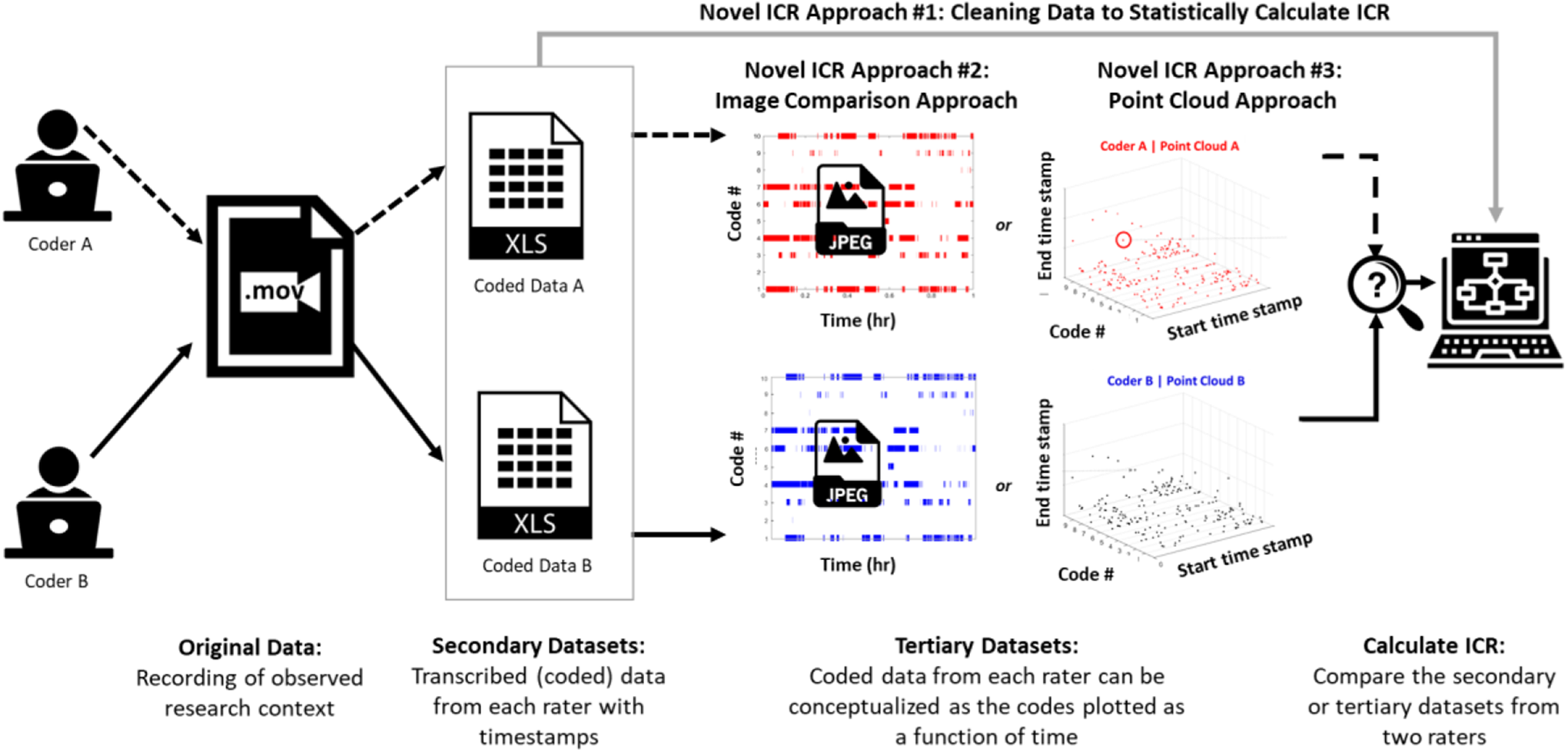
This paper demonstrates three novel ways to calculate ICR for observational data that has complexities, using secondary and tertiary representations of the observation in various formats. Novel ICR Approach #1 is an articulation of a cleaning procedure to account for complexities before applying traditional ICR calculations; Novel ICR Approach #2 uses image comparison methods to compare representations of the secondary coded data sets, and Novel ICR Approach #3 envisions the secondary data existing in a three-dimensional point cloud.

We then demonstrate our new methods applied to two separate ongoing research projects employing time-resolved observational video data. As a brief introduction, in the first research project, we collected screen capture and eye-gaze data from engineers performing a design task in the context of additive manufacturing to investigate research questions related to design cognition. In the second research project, we collected screen-capture data from engineering graduate students as they write an authentic research proposal to investigate research questions related to engineering writing behaviors. In both studies, we are interested in identifying how behaviors are distributed throughout the duration of observation. Using these two research contexts as platforms, we demonstrate how ICR can be performed using our methods, comparing their performance with ICR metrics calculated via traditional statistical methods for ICR.

Methods and Methodology for Calculation of Intercoder Reliability

In this section, we present three methods for cleaning data and subsequently calculating ICR. Throughout this paper, we consider each researcher’s coded data (with the corresponding timestamps) as a new secondary data set, such that the “data” and “data sets” to which we refer are the results of each researchers’ coding of some observational data (the secondary data sets, .xls files), not the raw observational video data itself (a single .mov file, in our case), as shown in Figure 2. The first method articulates the sequence of complex matrix manipulations involved in cleaning qualitatively coded data in observational studies so that ICR using traditional calculations (e.g., Cohen’s Kappa, Krippendorff’s Alpha) can be employed. The second and third methods are algorithmic methods that have not been considered to date in the qualitative methods literature. We performed each of these methods in MATLAB, a matrix-based data analysis program (.m files available upon request).

Novel ICR Approach #1: Cleaning Data to Statistically Calculate ICR in Overlapping, Time-Resolved, and Simultaneous Data

The first step in handling observational data is to assign a numerical value to represent each qualitative code, without assuming any priority or importance associated with the numerical value: To calculate ICR, it is necessary that all data be numeric even if it represents a theme or behavior. As an example, Figure 3 shows a generic example representing the outcome of two coders’ classification of some events or behaviors over a duration of time. The coders’ results contain overlapping codes and simultaneous event complexity. The duration over which each coder observed a given code (event or behavior) is represented as a generalized time-resolved matrix in Figure 3A and plotted as time-code bar graph in Figure 3B.

Figure 3.

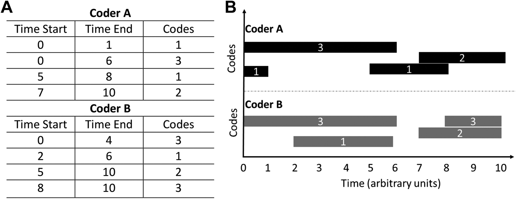
Generic coded data demonstrating: (A) matrix representation and (B) tick-bar plot for two coders’ data with Coder A data on bottom half and Coder B data on top half of the plot.

Partial agreement and simultaneous event complexities cause issues with respect to the foundational matrix theory by which ICR is typically calculated. To demonstrate our approach to cleaning these data, a generalized time-resolved data set (recall, this data set represents the coded data) can be represented as a matrix with first column as the start time stamp (S_i ), the second column as the end time stamp (E_i ) and third column as the numerical representation of code associated with the given time interval (C_i ), shown in Table 1. An event is defined as a time interval with unique code assigned and is represented as $[E_{i}, S_{i}, C_{i}]$ . If $E_{i - 1} = S_{i}$ , there is no overlap between sub-sequential events, and therefore is sequential time-resolved data. However, if $E_{i - 1} > S_{i}$ , there is an overlap between events. Therefore, to calculate ICR, the overlapping time event must be split into distinct non-overlapped events. As it is highly intensive to do this manually, we perform it algorithmically through the process described below. We refer to the first two columns, Time Start and Time End, as the time interval matrix.

Table 1.

Generalized Time–Resolved Data Matrix.

Time Start	Time End	Code
S ₁	E_i	C ₁
.	.	.
.	.	.
.	.	.
S_i	E_i	C_i
.	.	.
.	.	.
.	.	.
S_n	E_n	C_n

Matrix manipulation to eliminate complexities in simultaneous and overlapping codes

A four-step process is implemented to manipulate the data matrix and eliminate the complexities in the data sets, outlined through a logic flowchart in Figure 4. First, the algorithm eliminates simultaneous overlapping complexity by breaking overlapping codes at the timestamp where the overlap occurs, a process we call discretization. Then, the algorithm assigns the corresponding codes to these new discretized time intervals so that each discrete interval has one unique code. After the data sets of coded data from both raters are free from simultaneous overlapping complexity within their respective coding, we combine both matrices and employ a similar mechanism to eliminate the overlapping complexity, or partial agreement.

Figure 4.

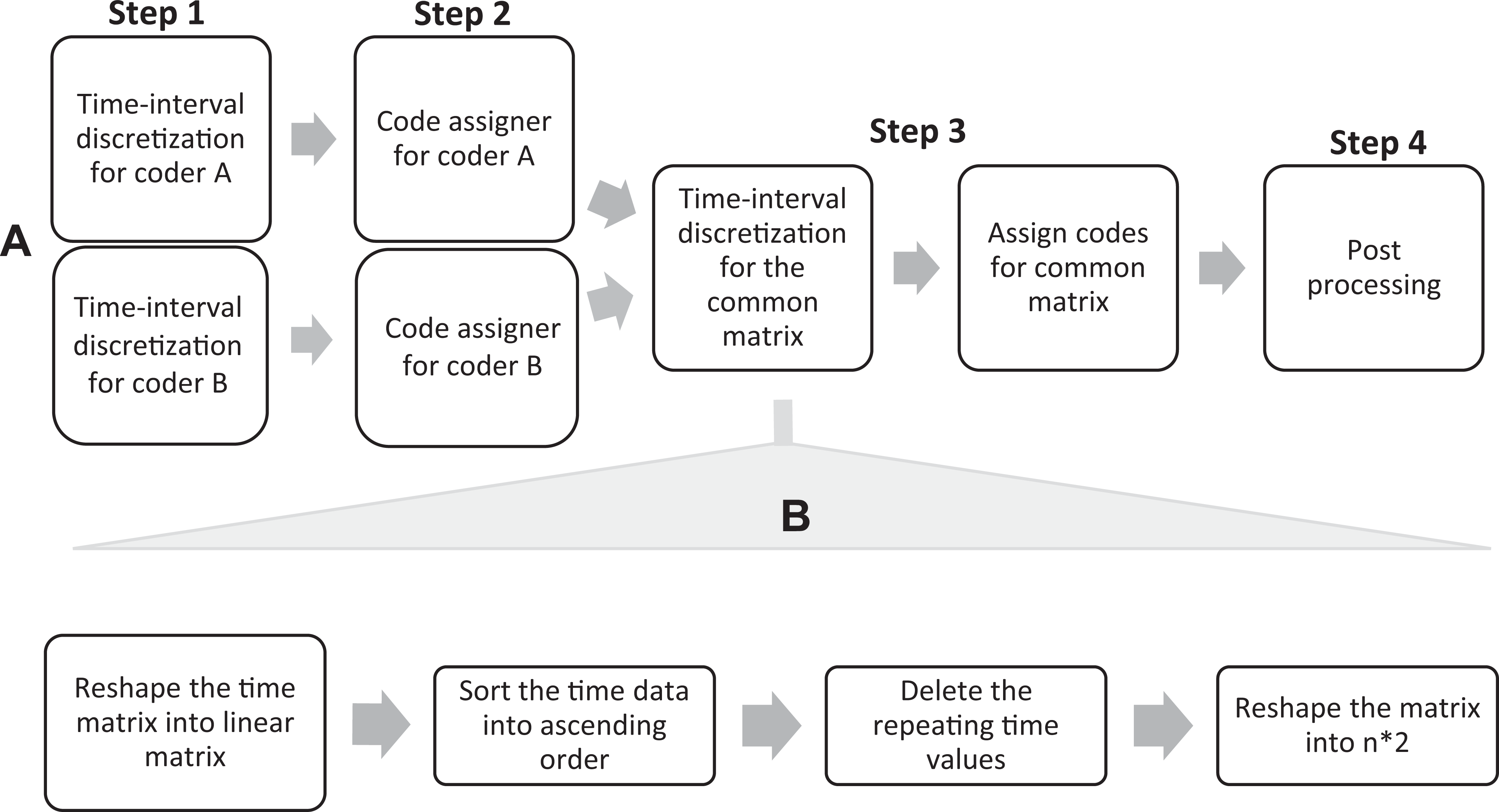
Logic flowchart for the algorithmic processes employed. (A) Four-step process to clean data to eliminate overlapping data categories. (B) Time interval discretization process.

Step 1: Time interval discretization for coders

Due to the presence of the simultaneous complexity in our data, time intervals of sequential events may overlap. To split the overlapping time intervals into discrete time intervals, we employed a four-step sequential matrix operation on time matrix from Figure 3B. First, the time matrix is reshaped into a linear matrix and then, the time values are sorted uniquely in an ascending order. The sorted matrix is reshaped into a new time matrix, with no overlapping time intervals. Figure 5 shows the implementation of time interval discretization on an example case for coder A.

Figure 5.

Demonstration of matrix manipulation to discretize overlapping time intervals.

Step 2: Assigning codes

To find the codes associated with new time intervals, we employed a grid search method. However, the process becomes more complex due to simultaneous events. To organize the data, codes for the same time interval are sorted in ascending numerical order, recalling that each numerical code stands for a qualitatively coded category or behavior. We selected a data threshold such that events occurring for very short time intervals (<2 seconds) were ignored. This threshold is a theoretical decision that depends on the research focus and the behavior of interest and can/should vary with context and research study based on methodological priorities of the researchers.

Step 3: Eliminating intercoder overlapping and partial agreement

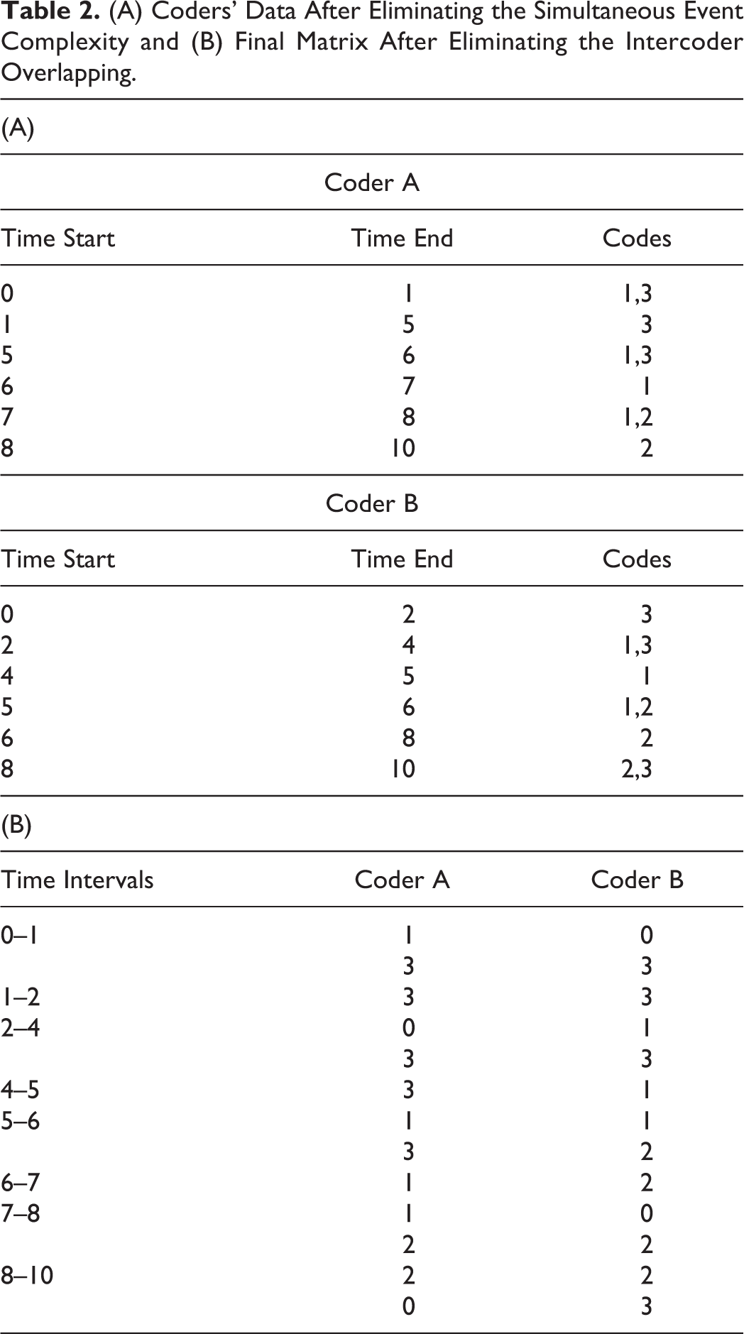
Due to unavailability of common unit size, time intervals of coder A and coder B are different and therefore, not directly comparable. To address the issue, we employ a similar two-step process of time interval discretization and code assigner, but with a common time matrix. Time discretization outputs a common time matrix, while a code assigner assigns the code to newly found time intervals for both coders (Table 2).

Table 2.

(A) Coders’ Data After Eliminating the Simultaneous Event Complexity and (B) Final Matrix After Eliminating the Intercoder Overlapping.

(A)
Coder A
Time Start	Time End	Codes
0	1	1,3
1	5	3
5	6	1,3
6	7	1
7	8	1,2
8	10	2
Coder B
Time Start	Time End	Codes
0	2	3
2	4	1,3
4	5	1
5	6	1,2
6	8	2
8	10	2,3
(B)
Time Intervals	Coder A	Coder B
0–1	1	0
0–1	3	3
1–2	3	3
2–4	0	1
2–4	3	3
4–5	3	1
5–6	1	1
5–6	3	2
6–7	1	2
7–8	1	0
7–8	2	2
8–10	2	2
8–10	0	3

Step 4: Determining ICR

Now that the data are no longer overlapping and have identical time intervals (there is no requirement for the time intervals to be evenly distributed, since we are operating from a critical events perspective), we can now use the resulting time matrix as the agreement matrix by which any statistical ICR calculation can be executed.

Mitigating Limitations of Statistical Methods for Time-Resolved Data

The limitation of a purely statistical approach to calculating ICR is that it is difficult to implement in practice, with a deep computational and statistical skillset required. In addition, this method is computationally expensive for larger data sets, due to the large number of matrix operations required. Instead, we propose two new methods to calculate ICR that leverage the fact that time-resolved data can be visualized spatially and then these representations can be compared algorithmically. These novel visual methods were first introduced in our previous work (Malviya & Berdanier, 2019) and have been modified in this paper to improve accuracy and mitigate paradoxes. While developing algorithms to create visual representations of coders’ results seems complex and time consuming, these two new methods are robust and can be applied quickly to other observational data sets once written. It can be argued that the statistical approaches are equally technically intensive to account properly for partial agreement and simultaneous data. We outline the logic by which comparison algorithms are developed.

Novel ICR Approach #2: Image Comparison Approach

Because the output of each coders’ results as a secondary data set can be visualized as a function of time graphically, we can use algorithmic methods to compare the visual representations of each coder’s results as a tertiary data set rather than working with the matrix of overlapping data in its raw form. In this approach, we envision the secondary data sets representing the coders’ results as tick-bar plots, with the categorical codes (behaviors) on the vertical axis and the time on the horizontal axis, as represented in Figure 3B. The images now constitute tertiary data sets representing the coders’ results that can be compared using image analysis methods instead. An example of these tertiary images that can be compared are shown in Figure 6. It is important to identify that as the algorithm manipulates the data, it is unnecessary to actually generate pictures unless the researcher seeks to explicitly envision the images during the process. In practicality though, the algorithm conducts the entire process without producing intermediate images for the researcher each time the algorithm runs unless desired.

Figure 6.

Example of tick-bar plot images, representing two coders’ results over time. The numerical code represents a categorical event or behavior, such that each occurrence of that theme is captured graphically on the images, which can then be algorithmically compared to calculate ICR.

Image comparison methods are common in computer graphics literature, using features like luminosity, structure, and contrast for comparison (Wang et al., 2004). For the purposes of this study, we are simply interested in ascertaining the structural similarity of the images representing two coders’ coding outputs. In our previous work, we compared raw images (cleaned of the unnecessary inclusions such as axes, legends, and colors) using the Structural Similarity Index Measure (SSIM), a common method for image comparison (Wang et al., 2004). However, we hypothesize that this method employed without standardizing the images results in inflated intercoder reliability due to noise from improper image resolution and missing pixels in the images. Furthermore, image processing tools do not allow precise control of image production. To overcome these issues, we take advantage of the fact that, in any programming language, an image can be represented as a matrix within which each cell represents the pixel value. To have better control on image generation, the time-resolved data is converted to a binary matrix where a value of zero represents the existence of an event, or the occurrence coded by coder during the time interval. This modified image comparison approach comprises three steps: resolution determination, sequential image conversion, and comparison.

Step 1: Resolution determination

Time-resolved data is graphically represented as two-dimensional tick-bar plot, with the x-axis representing the time stamp and the y-axis as the associated code, as shown in Figure 2B. The minimum y-axis resolution needed is equal to the number of the codes/categories in the time-resolved data. On the x-axis, every pixel denotes a shortest time interval. To perfectly capture the time-resolved data as a tick-bar plot, the shortest time interval should be equal to minimum time-interval possible ( $Δ t$ ) in both data sets. Using a user-defined minimum time-interval possible ( $Δ t$ ), the x-axis resolution, n, and the y-axis resolution, m, can be determined by Equation 1

m = # o f c o d e s, n = \frac{T}{Δ t} + 1

where T is the total time of the observational data.

Step 2: Image conversion

To generate a two-dimensional tick-bar plot from time-resolved observational data, we employ a sequential row operation consisting of three steps, as shown in Figure 7 for either of the coders (A or B). First, a dummy matrix of ones is created that has the resolution obtained from previous step (Step 1a). Concurrently, the time matrix of both data sets is converted into pixel- equivalent intervals (Step 1b). Second, a sequential row operation using a for-loop is employed and accounted for by a dummy variable k, which represents the row number. For any coded category n, a pixel lying between the pixel equivalent time intervals will be assigned zero in the nth row of the dummy matrix. For instance, the pixel equivalent time interval for the first row is [1,7] and the coded category is 3 (see Figure 4, Step 1b) Then, the pixels lying between 1 and 7 in the third row are assigned a zero, representing the event. This process is repeated until the end of the for-loop. This conversion process results in a smallest resolution image with more accurate representation of time-resolved data, reducing the computational cost. This process is repeated for the second coder.

Figure 7.

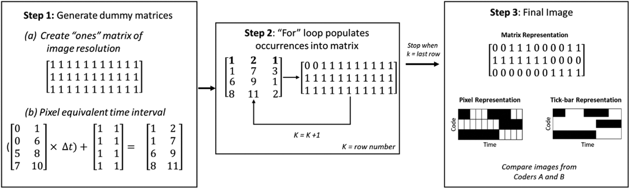
Image conversion and representation with one coder’s data.

Step 3: Image comparison

After generating both images, the last step is to compare the binary images. However, a direct image comparison will not be accurate due to interference from white pixels and reference image selection. In SSIM, white pixels are considered as an “event” in the image, thereby affecting the similarity percentage. Additionally, SSIM compares the deviation of a given image with the reference image, and thus it is important to select the correct image as reference. However, changing the reference image changes the similarity index drastically. Therefore, a new similarity algorithm is required to efficiently replicate statistical ICR calculations, which finds the similarity between two binary images (or plots). First, we add the image matrices from the two coders together. The resulting matrix has values of zero, one, or two. Here, the number of pixels with zero value (n ₀), represents the number of events in agreement, whereas the number of pixels with one value (n ₁), represents the number of events in disagreement. Pixels given a value of two represent the time intervals which were not considered as an event by either of the coders. This numbering is dependent on the numbering schema by which researchers indicate event occurrence in the matrix representation of the data (see Figure 6). We chose to represent event occurrence with a zero so as to reduce computational cost of rewriting the dummy “ones” matrix with each loop through the algorithm. The percentage agreement (p_a ) using this method is determined per Equation 2

p_{a} = \frac{n_{0}}{n_{1} + n_{0}}

Finally, the Brennan-Prediger formulation (Brennan-Prediger, 1981) is employed to calculate ICR accounting for chance agreement (Equation 3). The Brennan-Prediger approach to account for chance agreement was selected because it is independent of data type and depends only on q, the number of categories/codes:

I C R = \frac{p_{a} - \frac{1}{q}}{1 - \frac{1}{q}}

where p_a is the percentage agreement from Equation 2.

Novel ICR Approach #3: Point Cloud Approach

A second image-based approach is to represent the data in a three-dimensional point cloud rather than on a tick-bar plot. Building on our prior work (Malviya & Berdanier, 2019), each event of the time-resolved data is represented as a point in a three-dimensional space, with time start stamps and associated codes on the x- and y-axes, respectively, and the z-axis represents the end time stamp, thus creating a “cloud” of points in three dimensions, in other words, a 3-D point cloud. There are two data sets in our generic example, Data set A and Data Set B, representing Coder A and Coder B, so there will be two point clouds named Point Cloud A and Point Cloud B, respectively, as depicted in Figure 8A. To calculate ICR, we aim to find the similarity between Point Cloud A and Point Cloud B.

Figure 8.

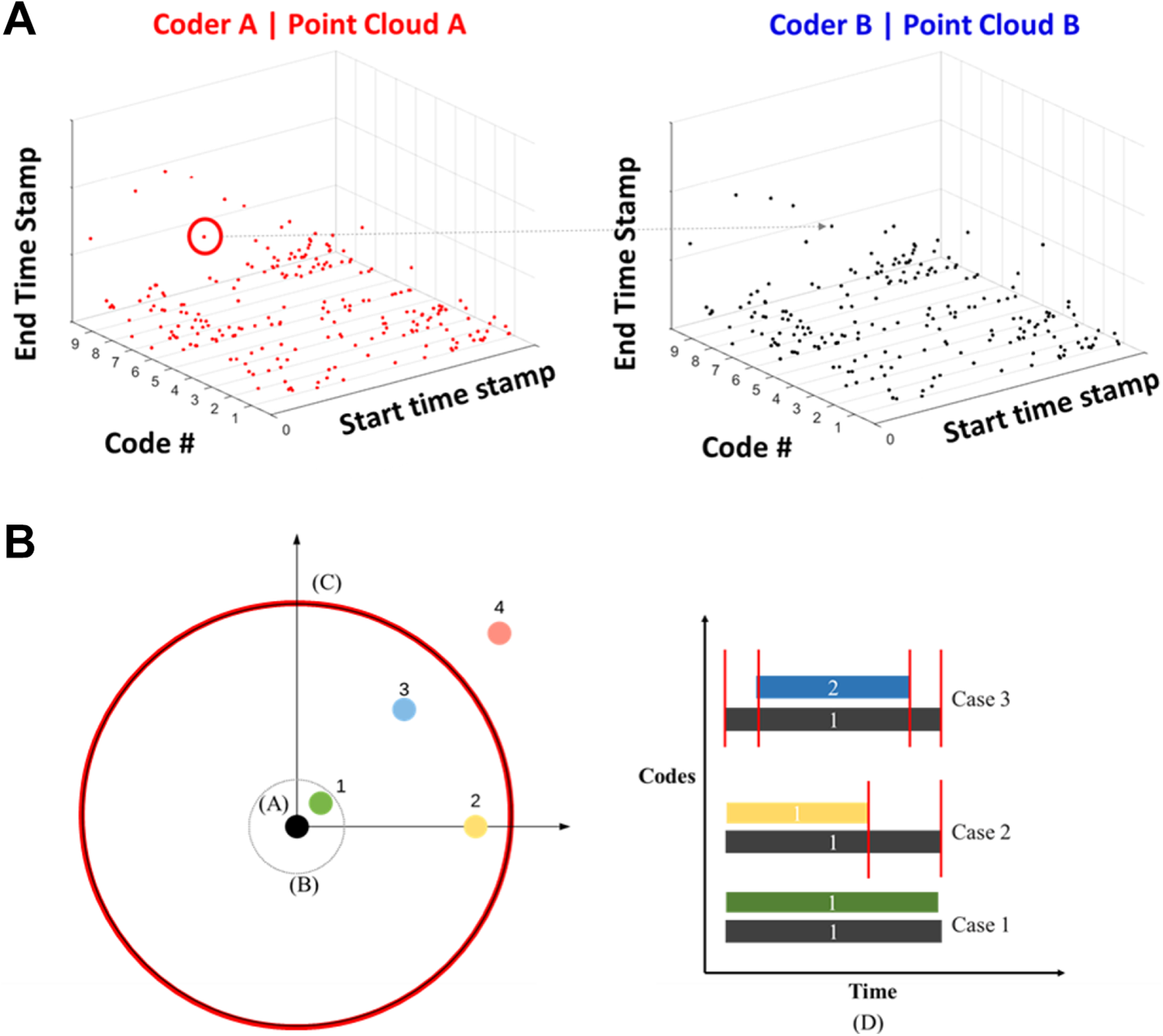
(A) Three-dimensional point cloud representation of a generic Data Set A within Point Cloud A mapped to Data Set B within Point Cloud B. (B) A two-dimensional “slice” of point cloud data. The black dot at location A represents Point t selected from Data Set A. The tolerance circle to account for lag between coders occurs at location B, and the duration circle representing how long a code lasts in Data Set A is shown at location C, having a radius equal to the duration of occurrence. The three cases by which overlapping data can be considered are depicted as points 1, 2, and 3. The representation of the three overlap cases of points 1, 2, and 3 is shown in location D.

Point cloud matching algorithms are popular in the field of computational graphics, especially for object detection, data retrieval, and modelling (e.g., Zhang et al., 2016), though we extend the algorithm into three dimensions. In our approach, we selected one reference point cloud to be the data set with the greatest number of events, and therefore points in the point cloud (for example, Data Set A). Figure 8 shows a diagram depicting the comparison of point clouds A and B and a 2-D slice of Point Cloud A to envision how the algorithm compares points: Systematically, a point t is selected from Data Set A, denoted in Figure 8 as the black dot in location A. Then, the algorithm searches Data Set B for the points in the category n that fall within a user-defined vicinity of point t selected. To accelerate the process, the user can bound the search space for the algorithm by defining a duration circle with radius $r = y - x$ as shown in Figure 8, at location C. If a suitable matching point is found in Data Set B, the algorithm updates a proxy counting variable (K) by one.

A tolerance circle is also defined to be agile in accounting for lag time between coders, as shown in location B. This threshold can be adjusted to reflect different tolerances—for example, researchers can decide whether coders rating the same code one second apart still can count as agreement, based on theory of the phenomenon of interest. In this way, the algorithm searches Data Set B for all the points lying in the duration circle for the same category.

In Figure 8, overlapping codes are denoted by points 1, 2, 3, and 4 (all in Data Set and Point Cloud A, recalling that this is a 2-dimensional “slice” of a 3-dimensional cloud of events. Point 4 lies outside of the duration radius and outside of the time-lag tolerance circle, so it is not considered as overlapping with point t. The search space for the algorithm will then contain all the points that exist in Data Set A that have an overlapping time interval with the point t. There are three possible cases: either the other point lies in the tolerance circle (Case 1, represented by point 1), lies on the one of the perpendicular axes (Case 2, represented by point 2), or lies anywhere else in the duration circle (Case 3, represented by point 3). Another representation of the three overlap cases as a function of time is shown in location D. In the computational algorithm, the number of matching points, denoted K, and the number of events, denoted E, is updated based on the case to which they belong.

Case 1 describes the scenario where similar events exist in Data Set B with possible time lag. K and E are updated as per the following expressions,

K = K + 1; E = E + 1

Case 2 describes the scenario where events have either same time start stamp or time end stamp. In this case, there will be two events after eliminating overlap (See Figure 8D, case 2). K and E are updated as per the following expressions,

K = K + 1; E = E + 2

Case 3 describes the scenario where an occurrence overlaps partially, with no common start or end point. In this case, there will be three occurrences after eliminating overlap with one matching occurrence, in which K and E are updated as per

K = K + 1; E = E + 3

This process is repeated for every data point until Data Set A has been searched in Point Cloud B.

To summarize the approach, Figure 9 represents an algorithmic logic flowchart for the Point Cloud approach, where K is the counting variable, E is the total number of events, C is the code number, and C_max is the total number of codes. The percentage agreement can be determined as the ratio of number of matching points found (K) and total number of points in Data Set A (E). The total event variable E is updated as per the Distance-Event Relationship to account for partial agreement and overlapping data. Then, percentage agreement can be defined as the ratio of total number of matching points (K) and total number of events (E). Then, as before, Brennan and Prediger’s method is implemented to account for chance agreement in calculating ICR using Equations 2 and 3.

Figure 9.

The algorithm flow chart for the 3D point cloud ICR approach.

Results: Performance of Novel Visual Approaches for ICR Compared With Statistical Methods

In the following section, we describe the application of the proposed ICR methods on two qualitative time-resolved data sets in engineering education research contexts. We test the performance of our two methods against five traditional statistical methods for calculating ICR after our data were cleaned for overlapping codes and simultaneous event complexity using the proposed procedures.

In our ongoing research, we study the quasi-cognitive processes of graduate engineering students as they undertake engineering design tasks and engineering writing tasks, with the goal of developing heuristic patterns to help graduate engineering students develop proficiency in engineering design and writing. We call these behaviors “quasi-cognitive” because the behaviors are indicative of cognitive processes but are not the direct cognition or electrical signals in the brain. As both design and writing are complex processes, having deep theoretical traditions in design theory (Atman et al., 2007; McComb et al., 2017; Pandey & Mourelatos, 2015) and composition theory (Flower & Hayes, 1981; Hayes, 2012) and respectively, we employed observational methods to capture time-resolved data of participants engaged in authentic design and writing activities. In this section, we introduce the readers to our two contexts to provide some contextual background, briefly describing data collection and analysis procedures. In both cases the primary observational data (video) is converted through the coding process by two raters into two sets of secondary data, the comparisons of which calculate ICR through the three proposed algorithmic methods.

For observational studies, there are several ways of interpreting video data to transcribe it in order to have time-stamped descriptions of the events/behaviors during the coding process. A very low-tech way to create time-stamped data is for each researcher to manually capture start time, end time, and code as they watch, stop, and start a video of an observational context. Technically, two raters could use this method to unitize and code data manually to capture it in excel before applying algorithmic methods to calculate ICR. However, this is obviously very time consuming especially to code long observation sessions and/or multiple participants.

In our both our observational studies, we used a manual method of transcription to develop and refine our codebooks, using theory in the respective contexts as starting points from which to modify the codebooks abductively. Then, to capture long durations of real-time observational data, we employed a touch-screen observational graphical user interface (GUI) developed by UC Davis, called the Generalized Observation and Reflection Platform (GORP) (UC Davis, 2020) to digitally capture which behaviors were occurring and when. The platform can be modified to reflect any codebook: As coders independently watch the screen recording, they tap the button on the interface representing the event/behavior they observe, and the platform captures the codes as a function of time. The GORP tool outputs an excel sheet of a coder’s observations and timestamps for any given observational session, comprising secondary Data Set A and Data Set B that are then compared (see Figure 2). This platform therefore enables real-time coding of observational video data.

Context 1: Investigating processes of engineering design for additive manufacturing

As a brief note on context, additive manufacturing (AM), related to 3D printing, is an emergent engineering technology leveraged across disciplines of engineering. Of interested to design theorists, Design for Additive Manufacturing (DfAM) theory is different from traditional Design for Manufacturing given the affordances and limitations of printing technologies and materials, but little is known how designers undertake the facets of DfAM throughout the duration of a design task. Therefore, one of the overarching research questions this study sought to answer was “What processes do designers undertake throughout a re-design for additive manufacturing design challenge?” A total of N = 9 graduate engineering student participants were recruited for this study. Each participant was tasked with re-designing a device for AM that had been originally designed to be manufactured through traditional methods given a variety of real-world design constraints. Each participant had 1 hr to finish the challenge. During the design challenge, the participants worked at a computer station equipped with relevant design software as well as eye-tracking and screen capture software. Thus, the participant’s entire design process was recorded by video that could later be analyzed by the research team. More details on findings from the study are available in our published work (Mehta, Berdanier et al., 2019; Mehta et al., 2020).

To develop the codebook by which to understand design processes, we leaned heavily on DfAM theory to capture the theoretically important incidents from a critical events perspective. Initial iterations of the codebook included potential behaviors that would capture each theme, translating DfAM theory (Booth et al., 2017) and design methods for Additive Manufacturing (e.g., Reddy et al., 2016; Schmelzle et al., 2015) and engineering design (Atman et al., 2007) into themes to serve as an a priori codebook. In initial rounds of codebook development, researchers employed a manual method of transcription whereby they slowly worked through video data, starting and stopping the recording manually, to record timestamps, observed behaviors, and capturing the representative codes. The constant comparative method through an abductive analysis approach (Timmermans & Tavory, 2014) was employed to determine whether new behaviors should be added to the codebook, or whether codes should be combined axially into an overarching category or removed. Similar codes were combined to reduce the number of codes, as the goal was to be able to eventually code in real-time. Removal of codes altogether occurred when the behavior was not observable on the screen (e.g., codes related to ideation or brainstorming, which are important parts of the design process, but are not “visible” through observation or eye-tracking). The research team was in discussion with researchers and other experts in Additive Manufacturing to ensure the relevancy and usefulness of the codebook related to DfAM principles.

Table 3 shows the finalized codebook developed to analyze the designers’ behaviors. Note that the qualitative behavioral codes are assigned a numerical value in order to employ our analysis. There is no ranking of the numerical codes (e.g., stress analysis, code 1, is not more important and does not necessarily occur before removing material, code 8).

Table 3.

Codebook for Observational Engineering Design Study.

Theme	Behavioral Code	Description	Code #
Verification	Stress analysis	Observing FEA results and performing stress analysis on created component	1
	Requirement/design prompt	Focusing on problem and objectives	2
	Inspection	Inspecting dimensions and considering AM restrictions	3
Composition	Add material	Adding new features	4
Composition	Sketching	Sketching	5
Modification	Revising	Smoothing existing features and using Fillet function	6
	Editing	Editing sketch, changing dimensions	7
	Remove material	Removing existing features	8

After codebook development, refinement, and iterative testing, the codebook was ready to deploy in conducting real-time observational coding for the video data captured from the nine participants (approximately 9 hr of data in sum). To analyze the recorded data, two coders employed the GORP tool, modified for this codebook, as an interactive digital codebook. As the video data captured each participant’s gaze point overtop the recording of the computer screen, the coders knew exactly to which behavior to code. Therefore, for this research context, we had no occurrences of simultaneous event complexity (e.g., the participants were not engaged in two behaviors at the same time.) Then, the output spreadsheets of timestamped codes were downloaded from the GORP tool by which ICR could be calculated.

Context 2: Investigating the writing process of graduate engineering students

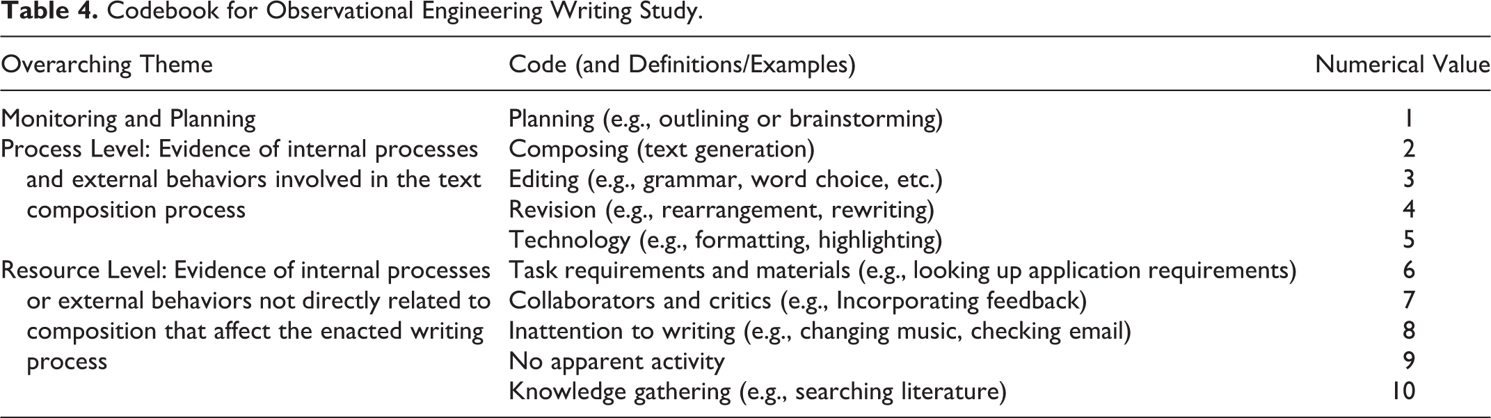
This study aims to characterize the time-resolved enacted writing behaviors and patterns of behaviors of engineering graduate students in authentic (non-classroom, non-contrived) writing settings. In this study, we collected screen-capture videos of the entire writing process of three graduate students who were writing research proposals and personal statements for a competitive national fellowship program. Initial codebook development was conducted by translating the Hierarchical Process Model of Writing (Flower & Hayes, 1981; Hayes, 2012) into a codebook of observable behaviors. One of the tenets of hierarchical process theories of writing is that writers can engage in more than one activity or behavior at a time, requiring the handling of simultaneous events in ICR calculation. Initial rounds of codebook development progressed through the transcription phase, by which two researchers manually recorded timestamps, summarized behaviors, and determined the representative codes. Philosophical decisions related to the transcription and codebook development process for these initial rounds can be found in prior work (Berdanier & Trellinger, 2017; Berdanier & Buswell, 2018). The constant comparative method through a post-positivist lens (Corbin & Strauss, 1990) using an abductive analysis approach (Timmermans & Tavory, 2014) was employed to determine new codebook behaviors, whether codes should be combined to reduce codebook complexity given goals of real-time coding, or removed altogether. Removed themes represented internal psychological (and therefore invisible processes) related to writing such as motivation, working memory, long-term memory, and reading, which are theoretically relevant but cannot be captured on a screen. Because we were interested in capturing the authenticity of the writing process, we expanded the codebook to capture non-writing elements such as listening to music or browsing the internet– tasks not affiliated directly with composition, but that are part of an authentic writing process. After iterative codebook development and testing, the finalized codebook presented in Table 4 was used to code the screen-recorded data captured from our three participants over dozens of writing sessions. In sum, this data set comprises over 40 hr of video observation data capturing the participants’ computer screens. Note that the codebook is formatted similarly to that of the design study codebook, with each code being assigned a numerical value.

Table 4.

Codebook for Observational Engineering Writing Study.

Overarching Theme	Code (and Definitions/Examples)	Numerical Value
Monitoring and Planning	Planning (e.g., outlining or brainstorming)	1
Process Level: Evidence of internal processes and external behaviors involved in the text composition process	Composing (text generation)	2
	Editing (e.g., grammar, word choice, etc.)	3
	Revision (e.g., rearrangement, rewriting)	4
	Technology (e.g., formatting, highlighting)	5
Resource Level: Evidence of internal processes or external behaviors not directly related to composition that affect the enacted writing process	Task requirements and materials (e.g., looking up application requirements)	6
	Collaborators and critics (e.g., Incorporating feedback)	7
	Inattention to writing (e.g., changing music, checking email)	8
	No apparent activity	9
	Knowledge gathering (e.g., searching literature)	10

As before, we programmed this codebook into the GORP tool, which was used to code data in real time to obtain time-stamped data for the two coders to be compared leveraging the three techniques presented in this paper.

Performance Comparison

We analyzed five statistical ICR methods in comparison to the two visual approaches proposed for our investigations. The results are shown in Table 5. Although the threshold for quality differs from context to context, most researchers follow guidelines in literature suggesting that an intercoder reliability (Cohen’s Kappa) of 0.41 to 0.6 is moderate, 0.61 to 0.80 is substantial, and 0.81 to 1 as almost perfect (with 1 being the maximum) (Gwet, 2008; Zapf et al., 2016). Other scholars (Fleiss, 1971) instead posit that Kappa values of 0.40-0.75 as fair to good, and above 0.75 as excellent. After calculating intercoder reliability, researchers must then use judgement to determine if the intercoder reliability is high enough to signify that the coding scheme is reliable across coders, or if further honing of the coding schema is required. For our studies, we achieved ICR in the moderate to substantial ranges, indicating our coding process is reliable but we may need to modify the code book or re-train the coders for more convergent results. For our contexts, which are not related to human health, slightly lower values of intercoder agreement may be acceptable.

Table 5.

Comparison of Calculated ICR Based on Statistical and Visual Methods.

	Context 1: Engineering Design Study			Context 2: Engineering Writing Study
	Percent Agreement (p_a )	Expected (Chance) Agreement Correction (p_e )	ICR	Percent Agreement (p_a )	Expected (Chance) Agreement Correction (p_e )	ICR
Statistical ICR Methods
Krippendorff’s α	0.6001	0.1639	0.5216	0.6965	0.1471	0.6445
Cohen’s κ	0.6001	0.1567	0.5257	0.6965	0.1444	0.6453
Scott’s Π	0.6001	0.1639	0.5216	0.6965	0.1471	0.6445
Brenan-Prediger	0.6001	0.1250	0.5429	0.6965	0.1	0.6628
Gwet AC	0.6001	0.1194	0.5457	0.6965	0.0948	0.6772
Visual ICR Methods
Novel Image Comparison	0.5626	0.1250	0.5002	0.7360	0.1	0.7067
Novel Point Cloud	0.5767	0.1250	0.5162	0.7782	0.1	0.7563

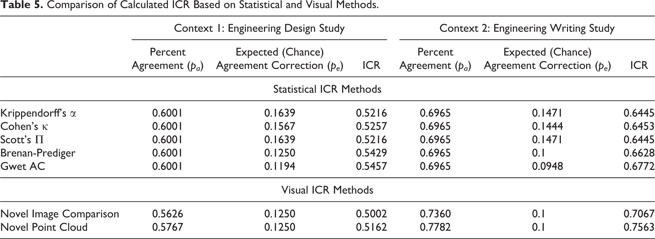
In these statistical methods, the variation comes primarily from the different chance agreement compensation. Findings indicate that the visual methods for calculating ICR are significantly close to statistical methods. In the Engineering Design study (Context 1), the ICR obtained through visual methods is lower than the computation of ICR from statistical methods, whereas in the Engineering Writing study (Context 2), the ICR obtained through visual methods slightly overestimates that calculated through statistical methods. This effect is due to the presence of simultaneous event complexity in the writing study, where the data is split into a greater number of events due to time-interval discretization.

The features and methodological choices of research manifest in the ICR results. For example, the ICR results based on the Point Cloud Approach for the Engineering Design Study was slightly more aligned with the statistical calculations of ICR, whereas the Image Comparison approach was more aligned with the statistical results for the Engineering Writing study. This difference manifests from the weighted nature of the Image Comparison Approach: The ICR obtained through image comparison accounts for every event differently in the final equation, which is more suited for the writing study from Context 2. For instance, an event with a duration of five seconds has a lesser effect on ICR than one lasting sixty seconds. In sum, our performance results suggest that our novel visual ICR methods can be implemented instead of spending significant time cleaning complex data for statistical methods after an appropriate algorithm for visual image comparison by either approach is developed.

Limitations and Future Work

As with any method, there are potential limitations that motivate future work. First, although we have translated this ICR approach to two of our ongoing research settings employing video data, there are opportunities to extend this method into other research contexts both employing video data and other forms of observational data. We would be interested to observe how these methods might be extended to other forms of digital data that are observational in nature but do not involve video data. We expect these novel visual methods would still be useful in ethnographic observations (if two raters are observing the same situation) as long as the research questions sought to observe how events/behaviors occurred as a function of time. We also expect the methods to be transferrable to any research context where two researchers are making an inference on whether a behavior has occurred as a function of time, where the reporting of ICR/IRR is essential to the rigor of the study. This would mean that some digital continuous data collection techniques (e.g., employing wearables to capture biological data) may benefit from this technique, dependent on both the data type and the research questions. If, in the example of wearables, coders were interpreting the continuous data to determine “when” something occurred that would vary between two raters (e.g., not a numerical threshold that could be computer-determined) then it could be useful. We welcome other researchers to employ and modify these approaches for their data and research needs, with the takeaway from our paper being the suggestion to think in creative ways to calculate ICR, rather than simply avoiding it.

A second limitation is that, like all ICR techniques including the classical approaches, there are statistical paradoxes that arise based on the algorithmic calculations, as established in literature (e.g., Gwet, 2008; Warrens, 2010). One example of a statistical paradox is when there are so few possible codes that the chance agreement between raters overwhelms the actual agreement. While the same statistical paradoxes arise from our methods because of the need to incorporate chance agreement, this is also an area of methodological future work that can be accomplished.

The final limitation we would like to address is simply the effort that is required to calculate ICR, either using traditional methods or our novel methods. In literature, the substantial effort required to calculate ICR has resulted in researchers either avoiding ICR altogether, perhaps using “social coding” methods as a work-around or substituting average metrics in lieu of precise agreements—none of which address partial agreement or simultaneous events. We acknowledge that there is effort required to both think through ICR calculations and to design/modify an algorithm in order to apply these novel approaches, and to clean and organize data to be analyzed computationally. For qualitative researchers uncomfortable with the calculations involve in calculating ICR for observational data or creating an algorithm to use image comparison approaches, we recommend partnering with other researchers who use data science methods to facilitate the process. However, we challenge qualitative researchers not to avoid ICR simply because it is difficult: is an unacceptable argument from a rigorous research perspective. Instead, ICR should be used as one method to promote quality in qualitative research, and our proposed methods now allow researchers to handle simultaneous events and partial agreement complexities. Further, calculating ICR for qualitative work, can mitigate the limitations presented by social coding (such as power dynamics between researchers) and can speak to the transferability of a codebook. Future work could include the development of an app or user-friendly computer program that could employ these methods without necessitating the modification of an algorithm.

Conclusion

In this paper, we articulated the processes required to accurately account for partial agreement and simultaneous event complexity that may occur when analyzing time-resolved observational data from a critical event perspective. This is the first paper to our knowledge that articulates the data manipulations required to employ traditional statistical methods of ICR, which are computationally intensive on the part of the researcher. As an alternative, we present two novel methods for calculating ICR using visualizations of two coders’ results to employ image comparison methods and a spatial point cloud search approach. Findings demonstrate successful calculation of intercoder reliability in our research contexts and high agreement between our novel visual methods and existing statistical methods. These methods are promising given recent technological advancements in high-resolution qualitative data collection tools for dynamic activity analysis within naturalistic or ethnographic, time-resolved observational research contexts. These are also the first methods proposed that are agile enough to handle partial agreement between raters, simultaneous event complexity, and enable researchers to set thresholds on time-lag agreement. In sum, this is the first paper that proposes re-envisioning ways to calculate ICR using visual methods, an advance that opens the opportunity to add quality to qualitative observational research.

Footnotes

Declaration of Conflicting Interests

The author(s) declared no potential conflicts of interest with respect to the research, authorship, and/or publication of this article.

Funding

The author(s) received no financial support for the research, authorship, and/or publication of this article.

ORCID iD

Natascha T. Buswell

Catherine G. P. Berdanier

References

Alford

B. L.

Rollins

K. B.

Padrón

Y. N.

Waxman

H. C.

(2016). Using systematic classroom observation to explore student engagement as a function of teachers’ developmentally appropriate instructional practices (DAIP) in ethnically diverse pre-kindergarten through second-grade classrooms. Early Childhood Education Journal, 44(6), 623–635.

Atman

C. J.

Adams

R. S.

Cardella

M. E.

Turns

Mosborg

Saleem

(2007). Engineering design processes: A comparison of students and expert practitioners. Journal of Engineering Education, 96(4), 359–379. https://doi.org/10.1002/j.2168-9830.2007.tb00945.x

Berdanier

C. G. P.

Buswell

N. M.

(2018, June 24–27). Data visualization for time-resolved real-time engineering writing processes. In 125th ASEE Annual Conference & Exposition, Salt Lake City, UT. American Society for Engineering Education.

Berdanier

C. G. P.

Trellinger

N. M.

(2017, October 18–21). Development of a method to study real-time engineering writing processes. In IEEE frontiers in education conference, Indianapolis, IN. IEEE .

Booth

J. W.

Alperovich

Chawla

Reid

T. N.

Ramani

(2017). The design for additive manufacturing worksheet. Journal of Mechanical Design, 139(10). https://doi.org/10.1115/1.4037251

Brennan

R. L.

Prediger

D. J.

(1981). Coefficient kappa: Some uses, misuses, and alternatives. Educational and Psychological Measurement, 41(3), 687–699.

Campbell

J. L.

Quincy

Osserman

Pedersen

O. K.

(2013). Coding in-depth semistructured interviews: Problems of unitization and intercoder reliability and agreement. Sociological Methods & Research, 42(3), 294–320. https://doi.org/10.1177/0049124113500475

Cohen

(1960). A coefficient of agreement for nominal scales. Educational and Psychological Measurement, 20, 37–46.

Corbin

J. M.

Strauss

(1990). Grounded theory research: Procedures, canons, and evaluative criteria. Qualitative Sociology, 13(1), 3–21.

10.

Derry

S. J.

Pea

R. D.

Barron

Engle

R. A.

Erickson

Goldman

Hall

Koschmann

Lemke

J. L.

Sharin

M. G.

Sherin

B. L.

(2010). Conducting video research in the learning sciences: Guidance on selection, analysis, technology, and ethics. The Journal of the Learning Sciences, 19(1), 3–53. https://doi.org/10.1080/10508400903452884

11.

Erlingsson

Brysiewicz

(2017). A hands-on guide to doing content analysis. African Journal of Emergency Medicine, 7(3), 93–99. https://doi.org/10.1016/j.afjem.2017.08.001

12.

Fleiss

(1971). Measuring nominal scale agreement among many raters. Psychological Bulletin, 76, 378–382. https://doi.org/10.1037/h0031619

13.

Flower

Hayes

(1981). A cognitive process theory of writing. College Composition and Communication, 32(4), 365–387. http://www.jstor.org/stable/356600

14.

Garrison

D. R.

Cleveland-Innes

Koole

Kappelman

(2006). Revisiting methodological issues in transcript analysis: Negotiated coding and reliability. The Internet and Higher Education, 9(1), 1–8. https://doi.org/10.1016/j.iheduc.2005.11.001

15.

Gwet

K. L.

(2008). Computing inter-rater reliability and its variance in the presence of high agreement. British Journal of Mathematical and Statistical Psychology, 61(1), 29–48. https://doi.org/10.1348/000711006X126600

16.

Hallgren

K. A.

(2012). Computing inter-rater reliability for observational data: An overview and tutorial. Tutorials in Quantitative Methods for Psychology, 8(1), 23–34. https://doi.org/10.20982/tqmp.08.1.p023

17.

Hayes

J. R.

(2012). Modeling and remodeling writing. Written Communication, 29(3), 369–388. https://doi.org/10.1177/0741088312451260

18.

Holley

J. W.

(1964). A note on the G index of agreement. Educational and Psychological Measurement, XXIV(4), 749–753.

19.

Jacob

R. J.

(1995). Eye tracking in advanced interface design. Virtual Environments and Advanced Interface Design, 258, 288.

20.

Klonek

Gerpott

F. H.

Lehmann-Willenbrock

Parker

S. K.

(2019). Time to go wild: How to conceptualize and measure process dynamics in real teams with high-resolution. Organizational Psychology Review, 9(4), 245–275.

21.

Knigge

Cope

(2006). Grounded visualization: Integrating the analysis of qualitative and quantitative data through grounded theory and visualization. Environment and Planning A, 38(11), 2021–2037.

22.

Knoblauch

Tuma

Schnettler

(2013). Video analysis and videography. In Flick

(Ed.), The Sage handbook of qualitative data analysis (pp. 435–449). Sage.

23.

(2011). A survey on behavior analysis in video surveillance applications. Video Surveillance. https://doi.org/10.5772/15302

24.

Koschmann

Stahl

Zemel

(2005). The video analyst’s manifesto (or the implications of Garfinkel’s policies for studying practice within design-based research. In Pea

Barron

Goldman

Derry

S. J.

(Eds.), Video research in the learning sciences. Taylor & Francis.

25.

Krippendorff

(1970). Estimating the reliability, systematic error and random error of interval data. Educational and Psychological Measurement, 30, 61–70.

26.

Long

Johnson

(2000). Rigour, reliability and validity in qualitative research. Clinical Effectiveness in Nursing, 4(1), 30–37.

27.

Malviya

Berdanier

C. G. P.

(2019, June 15–19). Visual and statistical methods to calculate interrater reliability for time-resolved qualitative data: Examples from a screen capture study of engineering writing patterns. In 126th ASEE Annual Conference & Exposition, Tampa, FL. American Society for Engineering Education.

28.

McComb

Cagan

Kotovsky

(2017). Capturing human sequence-learning abilities in configuration design tasks through Markov chains. Journal of Mechanical Design, Transactions of the ASME, 139(9), 1–12. https://doi.org/10.1115/1.4037185

29.

Mehta

Berdanier

C. G. P

Malviya

Miller

Manogharan

(2019). An empirical study linking additive manufacturing designers’ behaviors to success in manufacturability. In Solid Freeform Fabrication Symposium Proceedings, Austin, TX, August 2–4, 2021. The University of Texas.

30.

Mehta

Malviya

McComb

Manogharan

Berdanier

C. G. P.

(2020). Mining design heuristics for additive manufacturing via eye-tracking methods and hidden Markov modelling. Journal of Mechanical Design, 142(12), 124502. https://doi.org/10.1115/1.4048410

31.

Mezzich

(1981). Assessment of agreement among several formulating multiple diagnoses. Journal of Psychiatry, 16, 29–39.

32.

Pandey

Mourelatos

Z. P.

(2015). A new method for making design decisions: Decision topologies. Journal of Mechanical Design, Transactions of the ASME, 137(3), 1–8. https://doi.org/10.1115/1.4029218

33.

Powell

A. B.

Francisco

J. M.

Maher

C. A.

(2003). An analytical model for studying the development of learners’ mathematical ideas and reasoning using videotape data. The Journal of Mathematical Behavior, 22(4), 405–435.

34.

Reddy

K. S. N.

Maranan

Simpson

T. W.

Palmer

Dickman

C. J.

(2016, August). Application of topology optimization and design for additive manufacturing guidelines on an automotive component. In International design engineering technical conferences and computers and information in engineering conference (Vol. 50107, p. V02AT03A030). American Society of Mechanical Engineers. https://doi.org/10.1115/DETC2016-59719

35.

Rui

Feldman

J. M.

(2012). IRR (inter-rater reliability) of a COP (classroom observation protocol)—A critical appraisal. US-China Education Review B, 3, 305–315.

36.

Schmelzle

Kline

E. V.

Dickman

C. J.

Reutzel

E. W.

Jones

Simpson

T. W.

(2015). (Re) Designing for part consolidation: Understanding the challenges of metal additive manufacturing. Journal of Mechanical Design, 137(11). https://doi.org/10.1115/1.4031156

37.

Scott

W. A.

(1955). Reliability of content analysis: The case of nominal scale coding. Public Opinion Quarterly, 19(3), 321. https://doi.org/10.1086/266577

38.

Shweta

Bajpai

Chaturvedi

H. K.

(2015). Evaluation of inter-rater agreement and inter-rater reliability for observational data: An overview of concepts and methods. Journal of the Indian Academy of Applied Psychology, 41(3), 20–27.

39.

Tavory

Timmermans

(2014). Abductive analysis: Theorizing qualitative research. University of Chicago Press.

40.

Tong

Tang

Irby

B. J.

Lara-Alecio

Guerrero

(2020). The determination of appropriate coefficient indices for inter-rater reliability: Using classroom observation instruments as fidelity measures in large-scale randomized research. International Journal of Educational Research, 99, 101514.

41.

UC Davis. (2020). Generalized observation and reflection platform (GORP). https://cee.ucdavis.edu/GORP

42.

Waller

M. J.

Kaplan

S. A.

(2018). Systematic behavioral observation for emergent team phenomena: Key considerations for quantitative video-based approaches. Organizational Research Methods, 21(2), 500–515.

43.

Walther

Sochacka

N. W.

Kellam

N. N.

(2013). Quality in interpretive engineering education research: Reflections on an example study. Journal of Engineering Education, 102(4), 626–659. https://doi.org/10.1002/jee.20029

44.

Wang

Bovik

A. C.

Sheikh

H. R.

(2004). Image quality assessment: From error measurement to structural similarity. IEEE Transactions on Image Processing, 13(4), 600–612. https://doi.org/http://dx.doi.org/10.1016/j.future.2013.06.023

45.

Warrens

M. J.

(2010). A formal proof of a paradox associated with Cohen’s kappa. Journal of Classification, 27(3), 322–332. https://doi.org/10.1007/s00357-010-9060-x

46.

Werneke

Eccleston

Stephenson

MacFaul

Armon

(2003). Accounting for overlap? An application of Mezzich’s kappa statistic to test interrater reliability of interview data on parental accident and emergency attendance. Journal of Advanced Nursing, 33(6), 784–790. https://doi.org/10.1046/j.1365-2648.2001.01718.x

47.

Westbrook

J. I.

Ampt

(2009). Design, application and testing of the Work Observation Method by Activity Timing (WOMBAT) to measure clinicians’ patterns of work and communication. International Journal of Medical Informatics, 78(1), S25–S33. https://doi.org/10.1016/j.ijmedinf.2008.09.003

48.

Zapf

Castell

Morawietz

Karch

(2016). Measuring inter-rater reliability for nominal data—Which coefficients and confidence intervals are appropriate? BMC Medical Research Methodology, 16(1), 1–10. https://doi.org/10.1186/s12874-016-0200-9

49.

Zhang

Lin

Zhang

Wang

(2016). A fast method for measuring the similarity between 3d model and 3d point cloud. International Archives of the Photogrammetry, Remote Sensing and Spatial Information Sciences—ISPRS Archives, pp. 725–728. https://doi.org/10.5194/isprsarchives-XLI-B1-725-2016

50.

Hutson

Loschky

L. C.

Rebello

N. S.

(2017). Use of eye-tracking technology to investigate cognitive load theory. In Physics education research conference (pp. 472–475), Cincinnati, OH. https://doi.org/10.1119/perc.2017.pr.113

Visual and Statistical Methods to Calculate Intercoder Reliability for Time-Resolved Observational Research

Abstract

Keywords

Introduction

Calculating ICR in Observational Research: A Review of the Literature

The Purpose of This Paper: Contributing New ICR Methods for Observational Data

Methods and Methodology for Calculation of Intercoder Reliability

Novel ICR Approach #1: Cleaning Data to Statistically Calculate ICR in Overlapping, Time-Resolved, and Simultaneous Data

Matrix manipulation to eliminate complexities in simultaneous and overlapping codes

Step 1: Time interval discretization for coders

Step 2: Assigning codes

Step 3: Eliminating intercoder overlapping and partial agreement

Step 4: Determining ICR

Mitigating Limitations of Statistical Methods for Time-Resolved Data

Novel ICR Approach #2: Image Comparison Approach

Step 1: Resolution determination

Step 2: Image conversion

Step 3: Image comparison

Novel ICR Approach #3: Point Cloud Approach

Results: Performance of Novel Visual Approaches for ICR Compared With Statistical Methods

Context 1: Investigating processes of engineering design for additive manufacturing

Context 2: Investigating the writing process of graduate engineering students

Performance Comparison

Limitations and Future Work

Conclusion

Footnotes

Declaration of Conflicting Interests

Funding

ORCID iD

References