Cancer Risk Assessment and the Biostatistical Revolution of the 1970s—A Reflection

Abstract

Before around 1960, assessment of risk from exposure to toxic substances, including risk of cancer, was generally implemented using the NOAEL-safety factor approach that essentially assumed that an exposure threshold existed and exposures below the threshold carried no risk. In the 1970s there came a realization that cancer could develop from a mutation in a single cell and consequently it was unlikely that a threshold existed for substances that could cause such mutations, and that risk could increase linearly with exposure. During this time the Environmental Protection Agency (EPA) was formed and charged with protecting the public from a perceived high risk of environmental cancer. Faced with this difficult task, EPA decided to assess cancer risk by fitting a statistical model to dose-response cancer data and extrapolating to low dose using the fitted model. After some early experimentation EPA selected the Linearized Multistage Model for this fitting, which predicted risk increased linearly with exposure at low exposures. This approach led to an increased emphasis on statistical issues in risk assessment. Today, cancer risk assessment guidelines allow for different approaches depending upon the understanding of a substance's mode of action. However, a review of EPA's experience with current guidelines indicates that most cancer risk assessments still follow procedures similar to those initiated more than 40 years ago.

Introduction

I was invited to write this reflection because of my involvement in the development of cancer risk assessment methodology beginning in the 1970s. Thus, it is a highly personal account. It focusses on the Environmental Protection Agency’s (EPA) risk assessment practices as this agency was most prominent in developing and applying new approaches for cancer risk assessment during this time. This account also emphasizes the low-dose extrapolation issue since it is probably the most important and controversial one, and is the issue I was most involved in.

I graduated with my PhD in mathematics in 1968, and for a few years continued my research involving the theoretical mathematical model that had been the subject of my dissertation. But I began to realize that there were perhaps only 20 people in the world who were interested in this topic, and I resolved to move toward a topic that had promise of making a greater societal impact. Cancer risk assessment fulfilled this need very nicely.

The Early Days

Prior to around 1960, risk assessment for all adverse health effects, including cancer, were carried out in a similar manner. When based on animal data, as they mostly were, a no-observed-adverse-effect-level (NOAEL) was determined and divided by factors intended to account of the differences between animals and humans (the “NOAEL-safety factor” approach). The NOAEL was typically set at the highest experimental dose for which the toxic response was not statistically significantly greater than the response in control animals and was effectively assumed to be a dose that was risk-free in the animal species.

There are obvious shortcomings to this approach. It tacitly assumes that every toxic response has a threshold dose—a dose below which exposure has no effect on risk, even though demonstrating the existence of a threshold (which would entail proving a negative) is beyond the ability of science. In fact, by the 1960s scientists were beginning to doubt that such thresholds existed for certain effects, particularly cancers that could result from a mutation in a single cell. Also, a typical animal carcinogenicity experiment involved exposing no more than around 50 animals at each experimental dose. Such small numbers would not provide sufficient power to confidently detect a small increase in risk that would be of concern in a human population. For example, in an experiment involving 50 animals per dose group and 10 animals were found with a particular type of cancer in both the control group and a dosed group, it can only be concluded with 95% probability that the risk in the dosed group was no more than 0.08 greater than the risk in the control group (ie, a 95% upper confidence bound for the additional risk in the dosed group compared to the risk in the control group is 0.08.), and this large an increase in risk would be of serious concern in a human population.

The Mantel-Bryan (1961) Procedure

As a way around this conundrum, Mantel and coauthors ^1,2 proposed a method for calculating “safe doses” for carcinogens using a high- to low-dose extrapolation procedure that did not involve the assumption of a threshold. Although the Mantel-Bryan method apparently was never used by a regulatory agency to assess risk, it did break new ground by assuming a nonzero increase in risk at every dose, no matter how small the dose.

There were several conservative assumptions built into the Mantel-Bryan procedure. It employed a log-probit dose–response with no threshold. The probit slope was not estimated but was “conservatively set” at 1 normal deviate per 10-fold dose increase. A safe dose was defined as one corresponding to the tiny increased risk of 1/100 million. And a 99% statistical lower bound on the safe dose was recommended. However, despite these conservative assumptions the Mantel-Bryan method cannot be considered conservative. ³ It is instructive to examine the method to see why that is the case.

Figure 1A shows a graph of the Mantel-Bryan log-probit dose–response applied to the following data (dose, #tumors/ #animals): (0, 5/50), (25, 4/50), (50, 7/50), (100, 35/50). The Mantel-Bryan curve does appear to be conservative in this graph, as its predictions lie above the cancer responses at the lowest 2 doses. It also appears to be curving downward everywhere. However, if we use a magnifying glass to examine the Mantel-Bryan curve in the neighborhood of zero dose (Figure 2B), we see that the curve curves upward in the low-dose region (actually for doses, d, such that the additional risk (P(d) − P(0)) is less than 0.01), ⁴ the opposite of what appears to be the case in the unmagnified graph. The first derivative is zero at zero dose, so the model is, by definition, not low-dose linear (note 1), which also is not apparent in the unmagnified graph. Not only is the first derivative zero at zero dose, but derivatives of all orders are zero at zero dose (note 2). Thus, it could be called “super flat” at low dose. The principle problem with using the Mantel-Bryan curve to estimate low-dose risk is that there is no known biological mechanism that would produce a dose–response with this property.

Figure 1.

A, Illustration of the Mantel-Bryan (1961) dose–response extrapolation model fit to data shown (dose, #tumors/#animals): (0, 5/50), (25, 4/50), (50, 7/50), (100, 35/50), with 95% confidence intervals shown for the response at each dose. Solid curve is the Mantel-Bryan maximum likelihood curve. Dotted curve is the Mantel-Bryan upper confidence limit curve. B, Same as A except showing only the upper confidence limit curve at very low doses.

Figure 2.

Illustration of Carcinogen Assessment Group’s (CAG) original linear extrapolation approach using same data as in Figure 1. A straight line was drawn from the response at zero dose to the response at the lowest dose that was significantly greater than the response at zero dose.

The 1960s and 1970s

There was a lot of environmental activity in the 60s and 70s. Rachel Carson’s book, Silent Spring, which was published in 1962, was widely disseminated, and alerted the public to the possible detrimental effects of the indiscriminate use of pesticides. Also, during this time, it was estimated that as much as 90% of human cancers were caused by environmental agents. ⁵ This heightened public and scientific concern presaged the formation of the National Institute of Environmental Health Sciences (NIEHS) in 1969 and the EPA in 1970. President Nixon’s War on Cancer, which was initiated in 1971, followed closely.

And then in 1977, the Safe Drinking Water Committee of the National Research Council ⁶ published a highly influential report, entitled Drinking Water and Cancer, which reflected an emerging understanding of how many environmental cancers were initiated. This report concluded that for carcinogens “There is no scientific basis for…time-honored practice of classical toxicology is the establishment of maximal tolerated (no-effect) doses in humans based on finding a no-observed-adverse-effect dose in chronic experiments in animals, and to divide this dose by a ‘safety factor’ of, say, 100, to designate a ‘safe’ dose in humans.” Thus, the then-current practice of classical toxicology was deemed to be inappropriate for carcinogenic risk. The report also proposed a specific alternative for assessing carcinogenic risk: For “genetically self-propagating effects, for example, somatic or germ-cell mutation that culminates in a malignant neoplasm or is transmitted to later generations: Assume no threshold, assume a linear dose–response at low doses, and estimate risk.” The NRC Committee illustrated this approach to estimating low-dose risk by applying the multistage model of cancer to animal data on several chemicals. ^6,7 Regarding thresholds, the NAS report concluded that “Methods do not now exist to establish a threshold for long-term effects of toxic agents.” Note that this conclusion applied to all long-term toxic effects, not just cancer.

During 1974 to 1975, I spent an academic year as a Visiting Scientist in the Biometry Branch of NIEHS at the invitation of David Hoel, the branch chief. Soon after arriving there, I discovered that interest was growing in developing new methods for conducting cancer risk assessments that took account of the emerging ideas about the mutation origin of many chemical-induced cancers. I concluded that this was an important problem, and one to which I could profitably devote my attention. During that year, David Hoel, Chuck Langley, and myself at NIEHS and with the participation of Richard Peto in England, wrote a paper that examined several mathematical models of carcinogenesis with emphasis on their low-dose risk implications. ⁸ These models generalized the Armitage and Doll ^9–10 and Nordling ¹¹ cancer models by introducing the effect of dose rate into the models following Neyman and Scott. ¹² It was shown that the dose–response for these models would be linear in dose for small dose rates, except in highly specific cases unlikely to occur in practice. The article also derived bounds in special cases for the error in approximating the dose–response by a completely linear model.

Perhaps more importantly, this article introduced the “additive to background” rationale for linearity. This rationale noted the importance of background carcinogenesis to the shape of the dose–response curve at low doses, and showed that, “if carcinogenesis by an external agent acts additively with any already ongoing process, then under almost any model the response will be linear at low dose.” It is important to note that this rationale applies, not just to cancer, but to any health effect for which the stated conditions are satisfied.

At my very last day at NIEHS, upon the completion of my academic-year-long appointment, I had the very good fortune of meeting my replacement, Harry Guess. That day Harry grilled me about interesting projects I had found at NIEHS that he might work on. Among those we discussed were statistical problems related to assessment of low-dose risk from carcinogens. This meeting was the beginning of a collaboration between Harry and myself, with Harry usually taking the lead, that resulted in several publications on this topic, ^{13 -17} and produced what became known as the “Linearized Multistage Model” (LMS) for cancer risk assessment.

Environmental Protection Agency’s Early Approaches to Quantitative Risk Assessment for Carcinogens

And about this same time the relatively new agency, EPA, was grappling with the problem of how to protect the public from a perceived high risk of environmental cancer. The Agency had to determine which chemicals posed a cancer risk and how stringently to regulate them. This called for so some way to estimate the cancer risk from specific exposures. This was a very daunting job, and it still is. It was also a very controversial job, as an aroused agricultural–chemical industry saw the possibility that a zero cancer-risk policy could put them out of business. ¹⁸ The Carcinogen Assessment Group (CAG) was formed within EPA and given primary responsibility for dealing with this issue. Roy Albert was the first chairman of CAG.

The CAG decided early on that they could not depend wholly on human data to quantify cancer risk. To do so would be equivalent to using humans as test animals. The only feasible way CAG could envision to quantify low-dose cancer risk was to fit a mathematical model to (usually animal) cancer data and extrapolate to low dose using the fitted model. But which model should be used? The Atomic Energy Commission had previously estimated the cancer risk from exposure to Strontium 90 and Iodine 139 using a linear no-threshold model. Albert argued that EPA would simply be following the precedent set by another government agency in selecting a low-dose linear approach. ¹⁸ Undoubtedly, the emerging scientific consensus reflected in the soon-to-be-released ⁶ water report also played a role. So, linear it was!

But which linear model should be used? According to the study by Albert, ¹⁸ CAG’s first risk assessments used a very simple linear extrapolation approach. They drew a straight line from the lowest dose at which the response was significantly greater than that in controls to the response in controls and used this line to estimate low-dose risk (Figure 2). This was certainly a straight-forward method. No computer was needed, only a straight edge and a pencil. But it also had some shortcomings. For one thing, no statistical confidence bounds on risk were obtained. Also, the method ignored a lot of data. In Figure 2, it gives the impression of overestimating low-dose risk.

Carcinogen Assessment Group also tried estimating low-dose risk by fitting the one-hit model to the data. This had the advantage over the strictly linear approach of using all the data, but it often did not fit the data adequately, as illustrated in Figure 3, where it overestimates risk at lower doses.

Figure 3.

Fit of the one-hit model to same data as in Figure 1.

To resolve this problem, CAG organized an informal meeting on February 21, 1980 and invited several statisticians, including myself, from around the country, each of whom had a statistical method for low-dose extrapolation. At this meeting the statisticians were asked to explain their extrapolation method and compare it with those of other participants.

As a result of this informal meeting, CAG adopted the multistage model, which together with the statistical procedure for calculating statistical upper bounds on low-dose risk, was termed the Linearized Multistage Model, or LMS, as its extrapolation model. The LMS was used by EPA for several years to assess risk from chemical carcinogens.

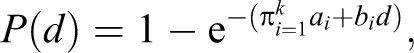
The multistage dose–response model is defined as

$P\left(d\right)=1-{\text{e}}^{-\left(q_0+q_{1}d+q_2{d}^2+\cdots +q_k{d}^k\right)},$

where d represents dose of a carcinogen and P(d) the probability of cancer when exposed to dose d, and the q’s are estimated parameters, all ≥0.

The multistage model is a generalization of both the one-hit model,

$P\left(d\right)=1-{\text{e}}^{-\left(q_0+q_{1}d\right)},$

and, the ^9,10 multistage model of cancer, modified to incorporate dose, ¹²

$P\left(d\right)=1-{\text{e}}^{-\left({\pi }_{i=1}^k{a}_i+b_{i}d\right)},$

where the a’s and b’s are all ≥0.

Both the multistage model and the Armitage-Doll model have an exponential polynomial form with nonnegative parameters. However, the multistage model does not contain all the restrictions on polynomials that the Armitage-Doll model contains.

The nonnegative restrictions on the parameters make the statistics associated with the multistage model very unlike standard regression. For example, it is not necessary to restrict the number of parameters to be less than the number of data points. The statistical theory behind the statistics associated with the LMS was worked out in a series of papers in the late 70s. ^13,14,16 Later it was discovered that confidence intervals derived from the asymptotic χ² distribution of the log-likelihood ^19,20 had improved properties over those based on the asymptotic normal distribution of the maximum likelihood estimates that were used in the earlier papers, and these confidence limits were used by EPA. ²¹

Figure 4 illustrates how the LMS model works. The solid curve is the multistage model, which, unlike the one-hit model (Figure 3), clearly provides a reasonable fit to these data. The dotted line in Figure 4 is the LMS, which also provides a reasonable fit. The linearized version incorporates a statistical upper upper bound on low-dose risk. It is calculated essentially by selecting the largest linear term, q ₁, consistent with the data, while adjusting the remaining parameters to achieve the best fit. Whereas the multistage model itself may not be linear at low dose, the linearized form is always linear. In fact, it contains the largest low-dose slope possible without significantly worsening the fit of the model. Thus, the LMS is not a model per se, but embodies a statistical confidence limit calculated from the multistage model.

Figure 4.

Solid curve is the fit of the multistage model to same data as in Figure 1. Dotted curve is the linearized multistage model (LMS) that determines the 95% upper confidence limit on added risk at low dose.

Figure 5 shows plots of the multistage, LMS, and upper bound Mantel-Bryan models for low doses for which risk is below 0.01, all based on the data shown in Figures 1 –4. The multistage model approaches zero as dose cubed (_∼ q ₃ × dose ³ because q ₁ and q ₂ are both estimated as zero with these data). The LMS approaches zero linearly (_∼ q ₁ × dose) because it contains the upper bound on q _{1 ,} which must be positive. Nevertheless, despite the divergence of these models at low dose, both fit the data adequately, as shown in Figure 4. The Mantel-Bryan upper bound lies above the LMS for doses corresponding to risk larger than around 10⁻⁵ but drops off much more rapidly than the LMS at lower doses. In fact, at still lower doses the Mantel-Bryan eventually fall below the multistage due to its extreme flatness at low doses.

Figure 5.

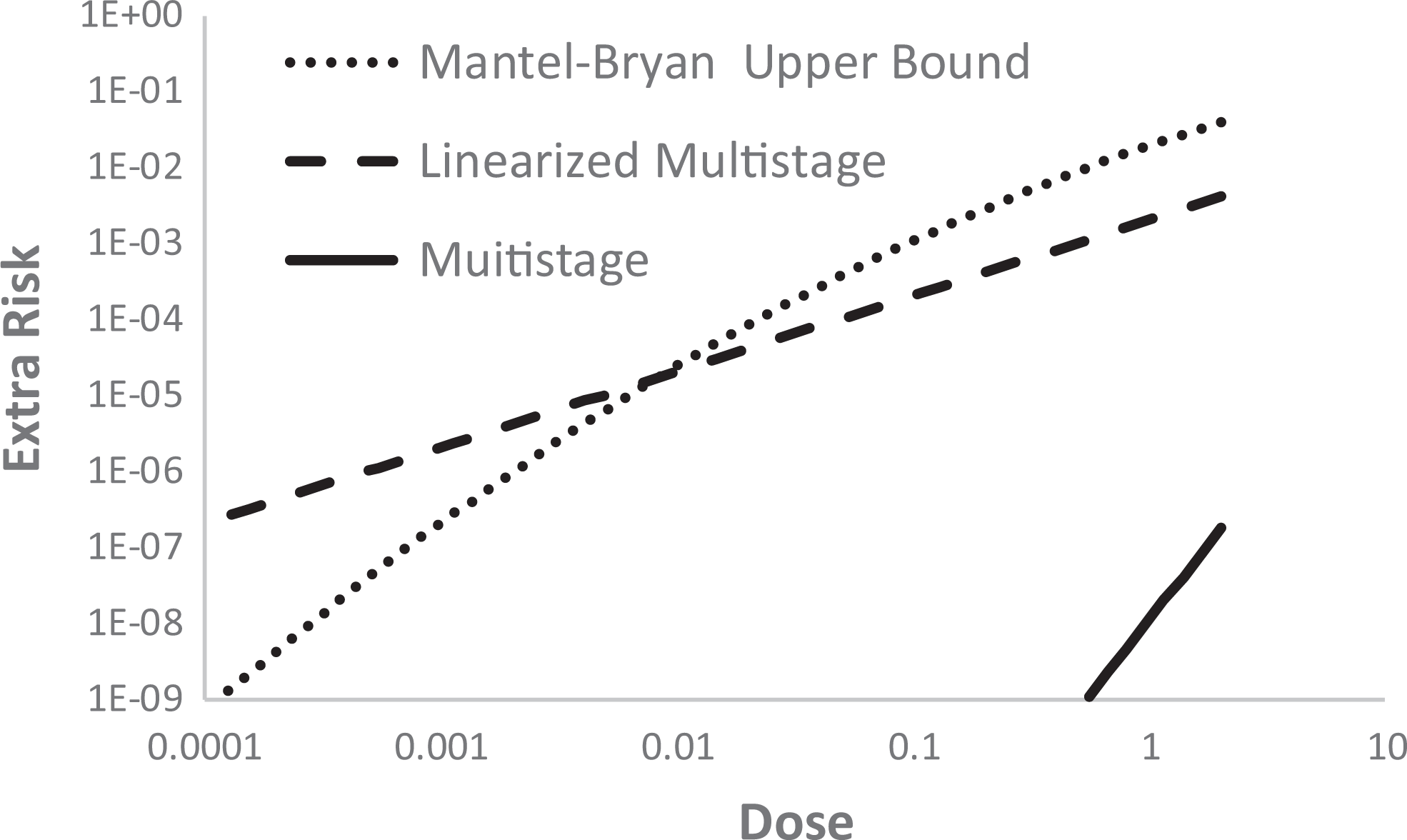
Graphs of the multistage, the linearized multistage, and the upper bound Mantel-Bryan model at low dose, all based on data shown in Figure 4.

To obtain an estimate of low-dose human risk from an animal study, it is necessary, in addition to performing low-dose extrapolation, to convert animal doses to equivalent human doses. By equivalent human doses are meant dose measures that are estimated to produce the same cancer risk in humans as were estimated in the experimental animals. The CAG accomplished this by assuming that mg/surface area per day, approximated by mg/[body weight]^2/3/day is an equivalent exposure in animals and humans. ²¹

Later Modifications

In the 1990s, EPA produced guidelines for risk assessment of several health effects. Among these were guidelines for reproductive toxicity ²² and neurotoxicity. ²³ Both of these documents allowed replacing the NOAEL in the NOAEL-safety factor approach with the benchmark lower bound (BMDL). ²⁴ The benchmark is defined as the dose corresponding to a prescribed increase (eg, 0.1) in the risk of an adverse outcome and is computed using a fit of a dose–response model to the dose–response data. The BMDL has several advantages over the NOAEL in safety assessment: Unlike the BMDL, the NOAEL depends only on the dose that is the NOAEL and does not incorporate information on the slope of the dose–response curve or the variability in the data. Smaller experiments (those with fewer animals per dose) will tend to give larger NOAELs, while the opposite is true of the BMDL. Thus, the BMDL more appropriately accounts for the greater evidence of safety resulting from more data. The NOAEL is limited to one of the experimental doses and consequently the number and spacing of doses can have an untoward effect upon the NOAEL. The NOAEL is often interpreted as a risk-free dose and, as noted earlier, this interpretation does not properly account for the power of the data to detect a response, and therefore is not defensible. The BMDL, however, being a lower bound on a dose corresponding to a prescribed increase in risk, is not subject to this interpretation.

Physiologically based pharmacokinetic models of the distribution, metabolism, and elimination of toxic chemicals in animals and humans were recommended to be used in extrapolating risks from animals to humans and across exposure patterns. ^22,23

Environmental Protection Agency’s 2005 Cancer Guidelines

In 2005 EPA produced cancer guidelines ²⁵ that made some fundamental changes in how cancer risk assessments are conducted by the agency. According to these guidelines, the preferred approach for cancer risk assessment is to use a toxicodynamic model, also known as a biologically based dose–response (BBDR) model, of the agent’s mode of action (MOA) and use that model for extrapolation to lower doses, if a suitable BBDR model is available. Biologically based dose–response models provide estimates of the probability of an adverse response, expressed as a function of biological variables involved in the response, such as cell division rates, death rates, and so on, that have physiologic meaning and, at least in theory, could be measured.

Lacking a suitable BBDR model, a statistical dose–response model (such as the LMS) is fit to the data and used to determine a “point of departure” (POD). The POD dose typically is a BMDL corresponding to a predetermined excess risk, for example, 0.1. Below the POD dose, risk is extrapolated to low dose using either linear extrapolation or “nonlinear extrapolation.” Linear extrapolation involves extrapolating linearly to low doses less than the POD dose and is used when there are data to indicate the MOA involves a dose–response having a linear component below the POD dose or as the default when the MOA is not established. Nonlinear extrapolation is used when there is sufficient data to ascertain the MOA and to conclude that the dose–response is not linear at low doses. Nonlinear extrapolation involves dividing the POD by safety or adjustment factors to obtain a reference dose (RfD) or reference concentration (RfC), and thus does not involve extrapolating a dose–response to low doses and does not provide an estimate of low-dose risk. Thus, the guidelines mandate a bifurcated approach, in which the extrapolation approach depends upon whether MOA information indicates a linear or nonlinear MOA.

Figure 6 illustrates the how this bifurcated approach is implemented. First, a BMDL is estimated using a statistical dose–response model (often apparently the LMS which was used for this step in Figure 6). This BMDL is a lower bound on the dose corresponding to a prescribed increase in risk (0.1 was used in Figure 6). This point (BMDL, 0.1) is the POD. If the MOA is determined to be linear or there is not sufficient information to determine the MOA, low-dose risk is estimated using the straight line shown in the figure. If the MOA is considered nonlinear, low-dose risk is not estimated. Instead the POD dose is divided by factors to arrive at an RfD or RfC.

Figure 6.

Illustration of low-dose cancer risk assessment under Environmental Protection Agency’s (EPA) 2005 guidelines using the same data as in Figure 1.

Thoughts About this History

It is interesting to see how the EPA 2005 cancer guidelines have been implemented in the 13 years they have been operational as of this writing. There has been deemed sufficient information to support a nonlinear MOA of action for only 2 chemicals, carbon tetrachloride and chloroform, and for carbon tetrachloride it was an alternative, and not the preferred approach (personal communication from EPA staff). Thus, it appears that, for the most part, chemical carcinogens continue to be regulated using a linear approach that is very similar to the one used by the EPA CAG in 1980.

Although the EPA 2005 cancer risk assessment guidelines permit use of a BBDR model, up to now no such model has been deemed reliable for low-dose risk estimation. Biologically based dose–response models replace the uncertainty in the shape of the dose–response for apical cancer at low doses with the corresponding uncertainty in the dose–responses for one or more intermediate steps in the cancer process, such as the division rate of cells. The dose–responses for these latter rates typically are no less uncertain than that for apical cancer. The data needed to develop a BBDR model, if available at all, generally cannot be obtained from the same group of animals, which causes problems associated with heterogeneity. The MOA being assumed will frequently be in question, as will the relevance of measurements to this MOA. Crump et al ²⁶ discussed difficulties with developing such models and concluded that “Difficulties in using BBDR models for [estimating low-dose risk] are conceptually the same as those faced when fitting empirical models to data on apical responses in intact animals. Moreover, these difficulties are exacerbated by problems inherent in complex models.” Their overall conclusion was “BBDR models are unlikely to be fruitful in reducing uncertainty in quantitative estimates of human risk from low-level exposures.” Therefore, it should not be surprising that, to date, no BBDR model has yet been developed that is deemed reliable for use in setting exposure guidelines (note 3).

Since cancer via a mutational mechanism has been generally agreed to likely have a linear dose–response, arguments for a nonlinear MOA appear to have focused on showing that the chemical is nonmutagenic. However, other MOAs could also lead to linearity at low dose. In particular, Crump et al ⁸ proposed the “additive to background” rationale for low-dose linearity. If a carcinogen acts by adding to a mechanism that is already producing background cancers, then the response will be linear at low dose. This rationale for low-dose linearity applies, not only to cancer, but also to any toxic effect that is adding to a mechanism that is causing the effect in background. For example, see Crump ²⁷ (Appendix B) for a description of how this mechanism could produce a linear dose–response in a population in which individuals have a threshold response mediated by inactivation of acetylcholinesterase molecules by covalent binding to an organophosphorus pesticide (In the last equation in this Appendix, the second P should be P′.). Seemingly, very little study has been directed toward this potential mechanism for low-dose linearity. As noted by a committee of the National Research Council, “EPA practices do not call for systematic evaluation of endogenous and exogenous exposures or mechanisms that can lead to linearity. ²⁸

In the 2005, EPA cancer guidelines, MOA information is used only to inform which of 2 risk assessment tracks to take, linear or nonlinear extrapolation. There are several conceptual problems with this approach. It is beyond science to determine conclusively whether a dose–response is low-dose linear or nonlinear. Mode of action information is not treated quantitatively. Other than its use in deciding whether to classify a carcinogen as linear or nonlinear, there is no relation between a MOA and the resulting RfD or RfC. Seemingly, a factor should be used to reduce the dose from the POD dose, which clearly cannot qualify as a risk-free dose, to a dose that is “safe enough” or below a threshold. Rather than treating all carcinogens deemed to have a nonlinear MOA the same, MOA information could be used in determining such a factor.

It is noteworthy that current cancer risk assessment practices bare close agreement with approaches employed 40 to 60 years in the past. On the one hand, if the MOA is deemed nonlinear, risk is assessed very much like it was assessed prior to 1970, the main difference being that the 2005 guidelines permit replacement of the NOAEL with the BMDL. However, proposals have been made for using probabilistic methods to replace the safety or adjustment factors in the nonlinear approach (eg, IPCS 2017). ²⁹ Probabilistic methods have also been proposed for addressing human variability (eg, Chiu and Slob 2015). ³⁰

Alternatively, if a nonlinear MOA cannot be established, risk is assessed using a linear model in a manner very similar to that used by CAG. The current approach calls for using a dose–response model (apparently often the same LMS model used by CAG in the 1980s) to estimate a POD and then extrapolating linearly downward from the POD. This should result in low-dose animal risks very similar to those obtained by CAG based on the LMS (although perhaps a bit higher, see Figure 6). Subramaniam et al ³¹ applied both approaches to 104 data sets and concluded that the 2 approaches provide estimates that are very similar.

Despite millions of dollars that have been spent on risk research, that effort has failed to resolve the shape of dose–response curves at low doses. After 70 or so years of research on radiation and cancer, there is still sharp disagreement on the shape of dose–response curves for ionizing radiation (eg, Crump). ²⁷ As noted above, current risk assessment practices are very similar to those employed many years ago. I believe that this state of affairs reflects a fundamental limitation in the ability of science to resolve critical questions regarding low-dose risk. Before meaningful progress can be made in improving risk assessment procedures, this fundamental limitation must be acknowledged and accommodated.