Sage Journals: Discover world-class research

Abstract

Costly and time-intensive trial-and-error sampling procedures plague traditional denim fabric production. This study develops and compares statistical and machine learning models to predict key properties of denim fabrics, aiming to reduce reliance on physical sampling in the textile manufacturing process. Models based on the two-level fractional factorial method using DOE, Random Forest (RF), and multilayer neural networks are constructed and rigorously validated using a real-world dataset comprising 1373 entries of denim fabric. Fabric properties, including before- and after-wash weights and thread counts, were accurately predicted. The neural network model demonstrated exceptional performance in predicting BW-EPI, achieving an R² of 0.979. In contrast, the DOE (multi-way) and RF models achieved strong prediction accuracy for AW-PPI, scoring R² of 0.971 and 0.969, respectively, accompanied by low MAE values (~0.77–0.90) and MAPE values (~1.34%–1.59%). The study further demonstrates practical user interfaces for both forward and reverse prediction, facilitating rapid, data-driven decision-making in denim production. Despite facing challenges in predicting fabric shrinkage due to dataset constraints, both statistical and machine learning models have proven highly effective for predicting fabric parameters, enabling data-driven decisions that improve resource utilization, enhance sustainability, minimize sampling trials, and accelerate development cycles.

Keywords

denim fabric fabric property prediction prediction models statistical methods design of experiments machine learning random forest artificial neural networks user interface textile manufacturing optimization

Introduction

Denim is a durable fabric predominantly crafted from cotton, known for its twill weave that produces a diagonal twill line effect. Classically, denim is made with indigo-dyed warp threads and undyed weft threads, which give it its distinctive appearance.¹ Innovations have introduced variations, including stretchable denim fabric. This fabric incorporates elastane, enhancing comfort and flexibility and allowing garments to fit closely without restricting movement.² Nowadays, Denim is a highly favored fashion choice because it is adaptable and suitable for people of all ages and throughout every season. It is used in the production of a diverse range of fashion items, including jeans, shirts, jackets, skirts, and more, for men, women, and children.^1,3,4 According to the latest statistics, the global market value for denim fabric was approximately $27.1 billion in 2022, with a forecast indicating that it will surpass $35 billion by 2027. This data shows sustained growth over the past period, with continued expansion driven by rising consumer demand and a diverse range of applications.⁵

To meet consumer demands, buyers introduced new trends and fashions every season; as a result, the R&D team frequently received inquiries from buyers about new fabrics with specific requirements.⁶ Initially, the manufacturer responds to the buyer by selecting fabric from its available archive and sending it to the buyer. If the buyer’s requirements are fulfilled, the fabric sample is acceptable. Otherwise, sample development is required to create a new sample, which involves different parameters that influence the physical and visual properties of the denim fabric. The R&D departments are responsible for setting fabric parameters based on previous experience and intuition. Then, the sample goes into the development stage. After completing the sample development, its properties are tested and compared with the buyer’s requirements. If the sample properties meet the buyer’s standard, the sample is ok. If not, a new sample is then produced and tested with the refined and modified fabric parameters. Usually, the sample fabric is ok after a large number of sample trials.⁷ Every case of sample fabric development involves raw materials, a workforce, and machines, making it expensive and time-consuming.⁸

Moreover, the properties of denim fabric, including weight, shrinkage, and twill line, are influenced by several structural and process variables, including yarn characteristics (e.g. thread counts and densities), weave type, fiber type, and finishing treatment. These parameters have complex relationships with the properties of the fabric.⁹ In sample development, the most crucial task is parameter selection, as it is directly correlated to properties. If the sample properties do not meet the buyer’s requirements, a new sample is made based on the previous one. This additional sample development places an undue burden on the industry and incurs extra costs.

In this context, techniques like neural networks (ANN)¹⁰ and random forests (RF)¹¹ are frequently utilized to support effective decision-making using available datasets. These methods are capable of identifying intricate associations between textile parameters and their resulting properties. Such machine learning methods enhance decision-making capacity by suggesting possible parameters and forecasting fabric properties, allowing for the determination of whether the developed sample meets the buyer’s requirements without requiring physical sample production. Zhenglei et al.¹² studied various intelligent modeling approaches, that is, ANN, RF, FL, support vector machines, and GEP, to analyze the relationship between parameters and the performance of the textile manufacturing process.

ANN demonstrated its usefulness in handling issues related to textiles of a broad range, including fiber-yarn relations, yarn and fabric properties prediction, fabric defects, and chemical processing.^13
–15 Specifically, Malik et al.¹⁶ presented a model using neural networks for forecasting and analyzing the permeability of air through woven fabrics made of polyester, concerning loom parameters, material, and weave. Their findings indicated that the passage of air through the fabric is determined by weave design and linear densities of yarn and filament, with variations of 10%–25% occurring due to machine dynamics. Katırcıoğlu et al.⁹ developed an ANN-based Artificial Bee Colony algorithm to predict quality parameters such as tensile, tear, and shrinkage of denim fabric concerning thread density and count, and the interlacing pattern between threads. Additionally, Zulfiqar et al.¹⁷ investigated a predictive model based on neural networks (ANN) on denim jeans for assessing the strength of used seams. The durability of denim jeans, as well as their quality, is significantly influenced by seam strength, which is determined by several key factors, such as the density of stitch, thread type and its linear density, and the areal density of the fabric, among others. Moreover, Bilisik and Demiryurek¹⁸ explored how the tensile-tear strength of abraded denim fabric is influenced by pattern using ANN. Zeydan¹⁹ introduced models like TDOE, ANN, and GA-ANN (neural networks comprising genetic algorithms) for predicting the resistance of fabrics to a longitudinal (tensile) force or stress, which are made using woven structures.

Furthermore, Kularatne et al.²⁰ applied both neural networks (ANN) and random forest (RF), considering the weave factor, count of longitudinal yarn, and density of traverse yarn to the fabric producing direction for modeling the modulus of elasticity of cloths made with woven architecture. The results show that both ANN and RF were able to produce accurate outcomes. However, RF was the better of the two models. Whereas Kastaci et al.²¹ introduced several models utilizing linear regression (multiple), ANN, and random forests for forecasting the braking strength of woven fabric. Seçkin et al.²² applied algorithms, including XGBoost, RF, and multi-layer perceptron (MLP), to predict weaving parameters and texture based on microscopic images.

The literature review revealed that ANN has been used for predicting yarn and woven fabric properties, but there have been very few studies on denim fabric. However, to the authors’ knowledge, no study has been found that used random forest (RF) and design of experiment (DOE) to predict denim fabric properties and interpret the separate and combined impacts of input parameters on these properties.

In this article, DOE and RF models are used to analyze the one-way and multi-way effects of input parameters on output fabric properties. Additionally, this research work proposes models using both statistical (DOE) and machine learning methods (ANN, RF) to develop a prediction framework for denim fabric properties, where input parameters are warp (Ne), weft (Ne), spandex (D), greige EPI, greige PPI, and color code, and output parameters are BW (before wash) weight, BW EPI, BW PPI, AW (after wash) weight, AW EPI, AW PPI, length shrinkage, and width shrinkage. Moreover, this framework can also suggest input parameters like greige EPI and greige PPI, based on the given fabric properties along with the parameters related to yarns. Finally, interactive user interfaces are developed to showcase the potential of using these frameworks from an industrial perspective.

Materials and methods

Materials

The production data for stretchable denim fabric were used in this experiment, where 100% cotton rotor or ring yarns were employed as warp yarns, and core-spun yarn (sheath: cotton, core: elastane) was used as weft yarns. For all the fabric samples considered in this study, the weave pattern was kept constant at 3/1 RHT (i.e. 3 up/1 down right-hand twill).

Fabrication process

In the broader context, rope and slasher dyeing are employed for dyeing the warp yarn in denim fabric production. For this article, production data were collected by researchers from a denim fabric manufacturer, that used the rope dyeing technique. Figure 1 Shows the process flow for producing denim fabric.

Figure 1.

Process sequence of denim fabric manufacturing.

The beginning phase of denim fabric manufacturing is the production of warp and weft yarn. The rope process begins with ball warping, where individual yarns are converted into ropes using a ball warping machine. After the ball warping, the ropes are passed through several dye boxes (depending on the shade) and dyed with dyestuff. The next step involves a long chain beam, where dyed warp yarn in rope form is converted into individual warp yarns and wound onto the beam for sizing.

Subsequently, the warp sheet passes through the sizing bath and is wound onto the sized beam. This process provides a warp yarn-protecting layer of size materials, which helps reduce yarn breakage. The obtained-sized beam is loaded into the loom (Air jet and Rapier). The output of the loom is greige fabric, which undergoes the “Desize finish” process and is converted into finished fabric. Desizing is carried out in hot water at 80°C. Following the quality inspection, the finished fabric is ready for dispatch. However, before dispatch, the lengthwise and widthwise shrinkage properties of the denim fabric are checked, which is carried out using soda, anti-back stain, and neutral agents.

Data collection & sorting

The data were collected from a renowned denim manufacturer in Bangladesh. A spreadsheet was provided, that listed all input and output parameters for each denim fabric produced by the company.

From that large dataset, researchers needed to extract the data for which prediction models were developed. Fabrics underwent a “Desize finish”, were made of cotton with spandex, and with 3/1 RHT weave type were chosen only. All these fabrics were colored using any of the following four types: Indigo, Black, Topping, and Bottoming. The effects of these color types on fabric properties are assumed to be negligible. Finally, a total of 1373 rows of data sets were extracted and used for this research work.

Development of a workable dataset

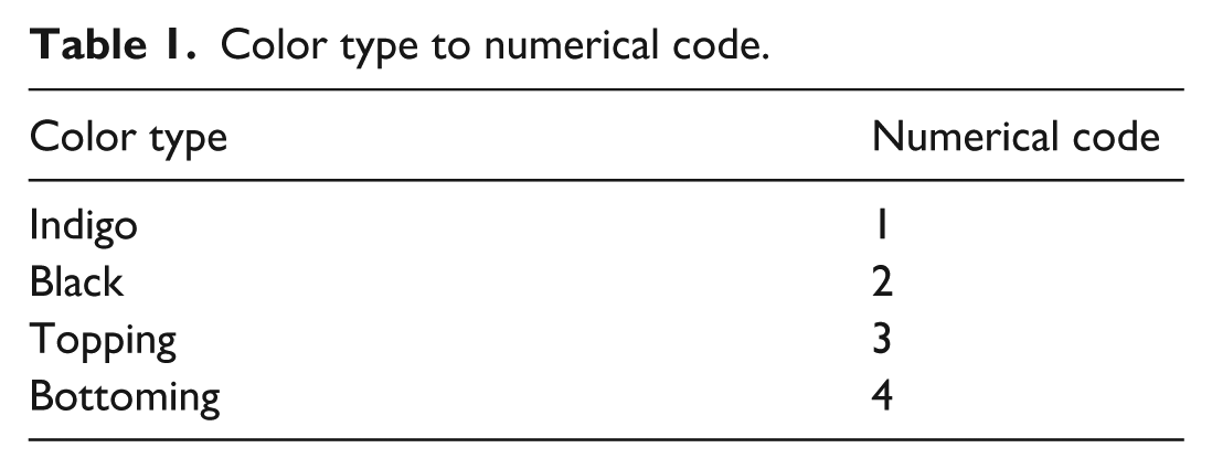
To utilize the dataset more effectively, several crucial steps were taken. The first important step was to calculate the resultant warp count (in English count, Ne), weft count (in English count, Ne), and spandex count (in Denier, D) from the warp ratio and the fabric construction columns of the original dataset. Then, the column of Gray, Finished, or After Wash EPI × PPI (Ends per inch × Picks per inch) was converted into two separate columns. The column of colors was transformed into numerical codes from the text values (Table 1), which facilitated the generation of prediction models.

Table 1.

Color type to numerical code.

Color type	Numerical code
Indigo	1
Black	2
Topping	3
Bottoming	4

Moreover, the after-wash fabric shrinkage percentage (which included both negative and positive values) was converted to the length of a 100 m fabric after washing. Finally, the workable dataset was developed (Table 2). Note that neither a single row of data was manipulated nor were assumed values put in any cell and the “Weaving code” column (refers to different fabric samples) was kept so that all the data can be traced back to the original spreadsheet provided by the company.

Table 2.

Sample of the sorted and formatted dataset.

Weaving code	Warp (Ne)	Weft (Ne)	Spandex (D)	Gray EPI	Gray PPI	Color code	BW weight	BW EPI	BW PPI	AW weight	AW EPI	AW PPI	AW length	AW width
16531 COS DF	7.40	10.00	40.00	56.00	40.00	3	11.38	70	49	13.06	78.00	44.00	98.75	87.80
16544 COS DF	8.00	16.00	40.00	66.00	52.00	1	11.08	76	58	12.00	87.00	59.00	98.28	87.00
16545 COS DF	8.00	16.00	40.00	60.00	44.00	4	9.96	77	49	12.09	88.00	51.00	95.20	87.67
16603 COS DF	16.00	16.00	40.00	88.00	46.00	3	8.82	112	50	11.59	140.00	53.00	94.92	79.60
16622 COS DF	8.00	16.00	40.00	60.00	46.00	3	10.29	77	51	11.98	89.00	52.00	99.50	88.29
18701 COS DF	8.00	16.00	40.00	60.00	45.00	3	9.96	76	49	11.67	85.00	51.00	98.50	87.87
16645 COS DF	9.00	16.00	40.00	66.00	52.00	1	10.17	82	57	11.7	92.00	59.00	96.25	89.60
16663 COS DF	18.83	20.00	40.00	83.00	60.00	1	7.84	118	65	9.7	140.00	69.00	96.87	82.95
16688 COS DF	8.66	16.00	40.00	71.00	52.00	1	11.59	80	59	12.53	92.00	60.00	98.74	89.24
16689 COS DF	8.66	16.00	40.00	66.00	52.00	1	11.23	76	58	12.23	87.00	59.00	99.14	85.62

Input and output parameters

To develop a prediction model using either a statistical method or a machine learning approach, the input and output parameters were first determined. For forward calculations, a total of six input parameters were taken, that is, resultant warp counts in English count (Warp (Ne)), resultant weft counts in English count (Weft (Ne)), spandex count in denier (Spandex (D)), ends per inch of gray fabric (Gray EPI), picks per inch of gray fabric (Gray PPI) and Color code. In Figure 2, it’s seen that for the output parameters, two layers were used where the first layer was for the output parameters before washing (BW) the fabric, that is, finished fabric weight (oz/yd²) before washing (BW Weight), ends per inch of finished fabric before washing (BW EPI) and picks per inch of finished fabric before washing (BW PPI). The second layer was for the output parameters after washing (AW) the fabric, where “AW Length” and “AW Width” represent the converted values of lengthwise and widthwise shrinkage, respectively, to the length of a 100 m fabric after washing the finished fabric. ISO 3801, ISO 7211-2, and ISO 6330 methods were used for determining the areal density (in g/m², which was converted to oz/yd²), yarn densities (EPI × PPI), and dimensional changes of the fabric, respectively.

Figure 2.

Input and output parameters (forward way).

Charts for effect analysis

Pareto chart and residual plots: A Pareto chart is a tool in statistics, used for finding and prioritizing input variables’ significance that influence the output variable in one or more ways. A reference line, at a 5% significance level (α = 0.05), which implies an input variable’s bar extending beyond this line, is considered to have a significant effect on the output variable.²³ Furthermore, residual plots are statistical tools used to assess the viability of a regression model. These charts were generated using the Design of Experiments (DOE).²⁴

Features importance chart: Presented in the form of a bar chart, this quantitative analysis highlights the significance (relative) of input variables in the prediction of the target variables. These charts are crafted for the Random Forest (RF) model, where the importance of features is assessed by the mean reduction in impurity across all decision trees.²⁵

Prediction models

For the prediction of denim fabric’s properties, both statistical and machine learning techniques were applied. The statistical method employed was the Design of Experiments (DOE), while machine learning approaches included the Random Forests (RF) and Neural Networks (ANN). The data was divided into two separate sets: one containing 85% of the total data (1167 records) for model training, and the other containing 15% of the total data (206 records) for model testing. This division was implemented to enhance the reliability of the comparisons between the outcomes of different models.

Design of experiments (DOE)

For planning, executing, evaluating, and interpreting, DOE, a systematic approach (statistical) is employed for controlled experiments that aim to assess the input variables that might affect a specific result or output response.²⁶ DOE (in Minitab software) offers several statistical techniques, among which the two-level fractional factorial technique was used in this research work, where every input factor is characterized by two levels, that is, high and low levels, and factorial regression is conducted either using one-way regression (Figure 3) or multi-way regression (Figure 4) for each output response.

Figure 3.

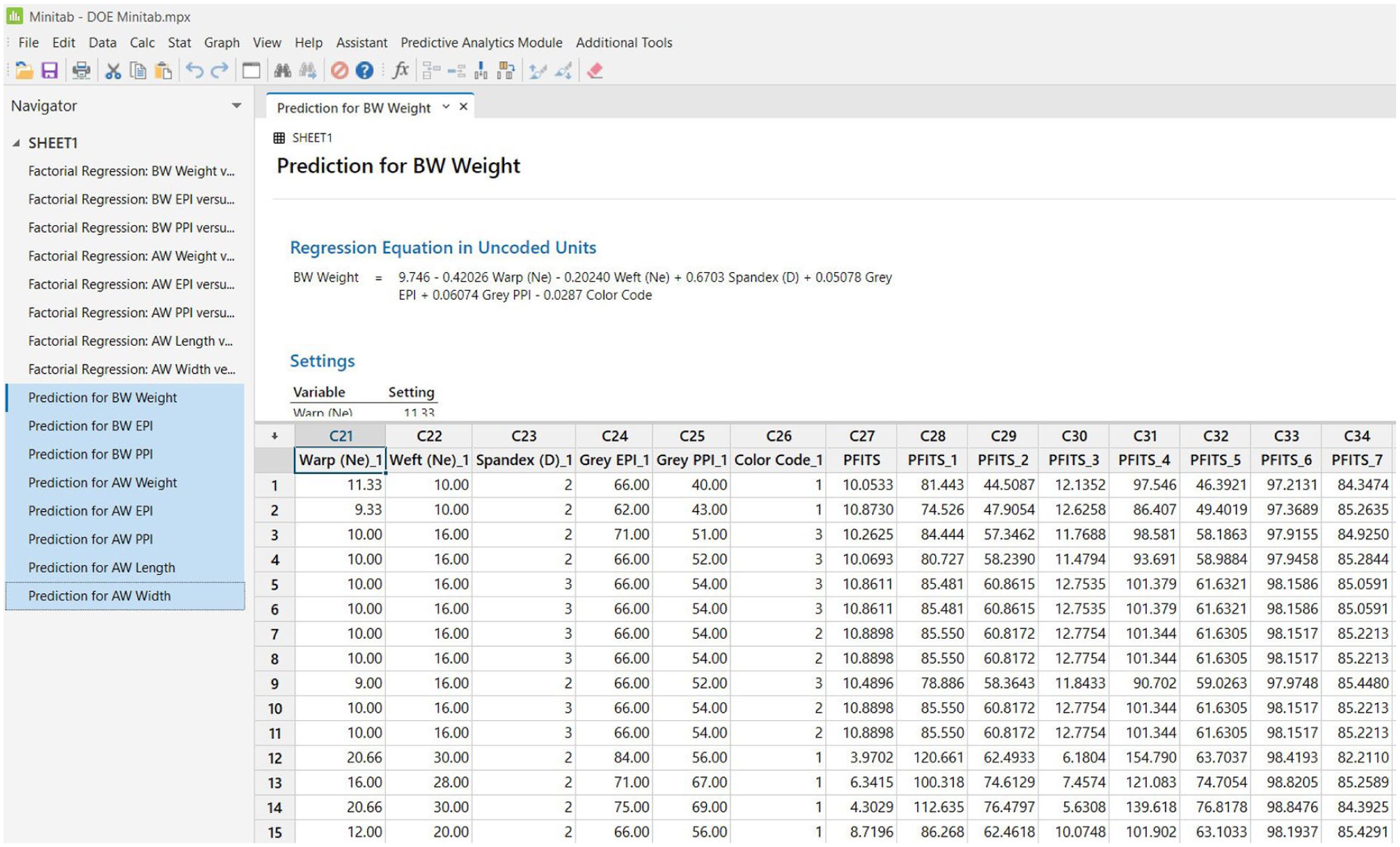
One-way (OW) regression using DOE.

Figure 4.

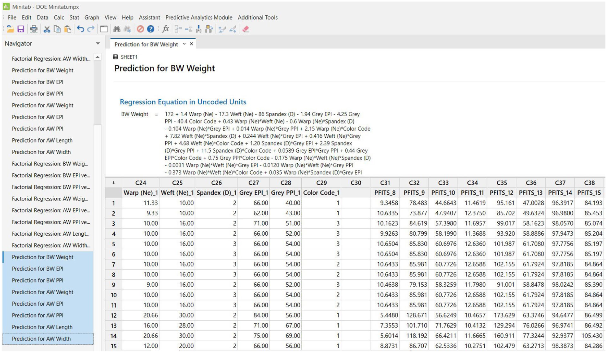
Multi-way (MW) regression using DOE.

Random forest (RF)

For tasks like classification and regression, Random Forest (RF), a supervised machine learning technique, is applicable. It functions by generating a multitude of decision trees and integrating their outputs to improve prediction accuracy.^27,28

In this experiment, the “RandomForestRegressor” module was utilized, which is part of the “ensemble” module in the widely used Python library for machine learning, “Scikit-learn.”²⁹

The same 85% training data and 15% test data were used for this model. Among the input parameters, the color code was characterized as a categorical variable. Figure 5 illustrates the pseudo-code of the RF model.

Figure 5.

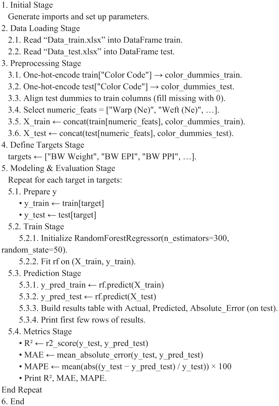
Pseudo-code of the RF model.

Different combinations of “n_estimators” (size of the forest, i.e. number of decision trees) and “random_state” (seed for randomness to ensure reproducibility) were used (24), for example, 100/40, 100/50, 300/40, 300/50, 500/40 and 500/50 among which n_estimators = 300 and random_state = 50 gave the best results. However, extensive hyperparameter tuning was not performed to avoid longer training/iteration time and model complexity. This approach provides a reproducible configuration with adequate accuracy and computation speed while avoiding over-parameterization.

Artificial neural network (ANN)

ANNs are computational frameworks that mimic the functioning of biological neurons, structured to handle information through a series of interconnected layers. Each artificial neuron receives inputs, assigns weights, and applies an activation function to generate significant nonlinear outputs. ANNs excel in identifying intricate patterns and understanding non-linear connections between input variables and their respective outputs, often surpassing the performance of conventional regression models.^15,28

The “MLPRegressor” module from the “neural_network” section of Python’s “Scikit-learn” library was employed to construct the ANN model, which is explicitly used for Multi-Layer Perceptron (MLP) regression tasks.²⁹

Figure 6 demonstrates a pseudo-code for the ANN workflow, which includes a preprocessing stage in which input normalization is performed prior to training. Numerical features are standardized using z-score normalization (StandardScaler), fitted exclusively on the training set and subsequently applied to both training and test sets to prevent data leakage. The categorical feature, “Color Code,” is one-hot encoded using OneHotEncoder(handle_unknown = (“ignore”) to maintain comparable input scales during ANN optimization. Additionally, Table 3 presents the values of each parameter along with their respective explanations used in the MLPRegressor code for developing the ANN model. The artificial neural network (ANN) architecture and hyperparameters were determined through a preliminary model selection process. Two-hidden-layer configurations with varying neuron counts, representing both reduced- and increased-capacity networks, were evaluated using the training set with internal validation. Model selection criteria included prediction performance (R², MAE, and MAPE), training stability, and computational time, as the final model was intended for deployment in a user interface where excessive computation time could negatively impact user experience. Deeper network architectures were excluded due to their increased computational demands. Of the evaluated configurations, the final architecture with hidden_layer_sizes = (64, 32) achieved the optimal balance between predictive accuracy and runtime efficiency, demonstrating improved performance metrics and stable convergence while maintaining acceptable computational time.

Figure 6.

Pseudo-code for the model using ANN.

Table 3.

Parameters for the ANN model.

Parameter	Meaning	Value used	Implication
hidden_layer_sizes	Specifies the structure (i.e., neurons) for internal layers in the ANN.	(64, 32)	The model consists of two layers: the first comprises 64 neurons, and the second includes 32, thereby defining the capacity.
activation	Determines the nonlinear transformation applied to neurons in hidden layers.	“relu”	Using the ReLU (Rectified Linear Unit) helps manage complex relationships and mitigates the vanishing gradient problem.
solver	Optimizer algorithm for adjusting model weights during training.	“adam”	The “adam” optimizer is well-suited for noisy or large-scale datasets due to its efficiency and adaptability.
alpha	Regularization strength (L2) to penalize large weights.	0.0001	A small alpha (0.0001) discourages overfitting by shrinking substantial weight coefficients.
max_iter	Maximum number of training iterations	1000	Training stops after 1000 iterations unless the model converges beforehand.
random_state	Controls the randomness for reproducibility	50	Ensure that results are consistent every time the code is run.

K-fold cross-validation

To validate the performance of the models based on machine learning, cross-validation (i.e. K-fold) is employed.³⁰ In this context, both the RF and ANN models underwent evaluation using 5fold and 10-fold cross-validation on the entire dataset without the described (Prediction models) train/test split. In 5-fold CV, the dataset is divided into five equal segments, with each fold utilizing 4/5 (80%) and 1/5 (20%) parts of the dataset, for training and testing, respectively. Conversely, 10-fold CV divides the data into 10 segments, training on 9/10 (90%) and testing on 1/10 (10%). The performance results are presented as the average and standard deviation of the R² (as well as MAE and MAPE) across the 5 or 10-folds.

Performance metrics

To evaluate model effectiveness, three key indicators were applied: R² (coefficient of determination), MAE (mean absolute error), and MAPE (mean absolute percentage error). For cross-validation, Standard Deviation (σ) was also used. The mathematical formulas for these performance metrics are provided below.²⁸

R^{2} = 1 - \frac{\sum_{i = 1}^{n} {(y_{i} - \hat{y_{i}})}^{2}}{\sum_{i = 1}^{n} {(y_{i} - \bar{y})}^{2}}

(1)

MAE = \frac{1}{n} \sum_{i = 1}^{n} | y_{i} - \hat{y_{i}} |

(2)

MAPE = \frac{100 %}{n} \sum_{i = 1}^{n} | \frac{y_{i} - \hat{y_{i}}}{y_{i}} |

(3)

σ = \sqrt{\frac{1}{n} \sum_{i = 1}^{n} {(x_{i} - \bar{x})}^{2}}

(4)

Here $y_{i}, \hat{y_{i}}, \bar{y}, n, x_{i}, and \bar{x}$ refers to the true outputs, estimated outputs, average actual values, total sample size, individual observations, and the dataset’s overall average, respectively.

For DOE, R² values were directly obtained from the software; however, it does not provide error metrics, such as MAE and MAPE. As a result, the predicted values were exported to Microsoft Excel, where the values of these two metrics were manually calculated using standard statistical formulas. However, for RF and ANN models, the “metrics” module was used for calculating all the performance metrics from the “Scikit-learn” library in Python.

Reverse calculations

In this segment, the same RF model or ANN model was used for prediction, but the input and output parameters were changed. A total of seven input parameters were taken, that is, Warp (Ne), Weft (Ne), Spandex (D), Color code, and either three before wash parameters (BW Weight, BW EPI, BW PPI) or after wash parameters (AW Weight, AW EPI, AW PPI). On the other hand, the targets were ends per inch of gray fabric (Gray EPI) and picks per inch of gray fabric (Gray PPI).

Development of user interface (UI)

To provide a demonstration of the application of these prediction models developed using random forest or artificial neural networks in the real-life world, two different (forward and reverse) user interface (UI) was developed using the “streamlit” library in Python. Figure 7 shows a pseudo-code for the forward-way user interface.

Figure 7.

Pseudo-code of forward UI using ANN.

Behind the UIs, .the predictive model, either a random forest (RF) or artificial neural network (ANN), is trained and evaluated using an online-stored dataset with a fixed 85%/15% train-test split (Figure 7). The model is fitted on the training subset and evaluated on the held-out test subset. The resulting test-set error, measured by mean absolute percentage error (MAPE), is reported as an “accuracy” metric (100−MAPE) to provide a benchmark of overall model performance. During user interaction, the user interface (UI) accepts production inputs within predefined thresholds, validates the entries, and utilizes the trained model exclusively for inference. User inputs are transformed using the same preprocessing pipeline, such as numerical scaling and categorical encoding, before being passed to the model to generate predicted outputs. User-provided inputs are not incorporated into the training or test dataset and are not used for retraining, as the corresponding target outputs are unavailable at the time of input. Model retraining is only necessary when the underlying stored dataset is updated with new labeled production records, which enables prediction performance to improve as the dataset expands.

Results and discussion

Significance of input variables on the fabric properties

Figure 8 illustrates a Pareto chart and residual plots for one-way regression in DOE, which aid in interpreting the significance of the six individual input variables on the BW (before wash) weight. From the Pareto chart (Figure 8), it is evident that Warp (Ne) has the most significant and dominant standardized effect. Weft (Ne) and Spandex (D) also have statistically significant effects, whereas Gray EPI and Gray PPI have low significance. On the other hand, the color code falls below their critical values, indicating it is insignificant. Similarly, it is possible to demonstrate the significance level of input variables for each output response. Refer to the Appendix (Appendix Figure 15) for individual Pareto charts that illustrate the standardized effects of one-way DOE.

Figure 8.

Standardized effects and residual plots from one-way DOE analysis.

Figure 9 illustrates how input variables simultaneously impact the BW (before wash) weight through multi-way regression in DOE. It shows that not only individual input variables but also possible different combinations of input variables have a statistically significant standardized effect on output variables, as the bar length exceeds the critical value. Among these combinations, the A × D (Warp Ne and Gray EPI) factor has the most significant standardized effect on the BW weight. Following the AD factors, B × D × E (Weft Ne, Gray EPI, Gray PPI) and D × E (Gray EPI, Gray PPI) have significant effects. Similarly, this model is capable of explaining the impact of the multi-way input variable on every output response. Refer to the Appendix (Appendix Figure 17) for the Pareto charts of standardized effects generated using multi-way DOE.

Figure 9.

Standardized effects and residual plots from multi-way DOE analysis.

Figures 8 and 9 also presents residual plots for BW weight in both one-way and multi-way regression, which are consistent with the fundamental assumptions of regression models. The probability plot (normal) indicates that residuals closely follow a normal distribution, adhering to the anticipated trend line. This is further supported by the histogram, which shows a nearly symmetrical shape centered around zero. Moreover, the plot of residuals against fitted values illustrates a random scattering of points around zero, with no discernible pattern, thereby confirming the assumptions of linearity and homogeneity. Moreover, the residuals versus order plot indicates independence, with no visible trend over time. The model for BW weight is sound and appropriate for prediction and interference. Refer to the Appendix (Appendix Figure 15 and 17) for residual plots for other output parameters.

Figure 10 displays a feature importance chart for the target BW Weight of the Random Forest (RF) model, indicating that Warp (Ne) is the most significant input variable, accounting for 71.6% of the total model significance in the BW (before wash) weight. Following this input factor, Weft Ne, at 9.4%, and Spandex (D), at 6.0%, showed a lower importance level. The color factor contributes to a negligible impact on BW weight. This trend is similar to the Pareto chart shown in Figure 8, which validates the accuracy of modeling for both DOE and RF. The significance of each input variable in relation to every output variable can also be assessed. Refer to the Appendix (Figure 16) for the bar chart illustrating feature importance.

Figure 10.

Feature importances of input factors on the outputs using the random forest model.

Prediction performance of different models

The research work analyzed how different models performed in predicting various denim fabric properties, using two modeling approaches: statistical method, which included one-way (OW) regression and multi-way (MW) regression using Design of Experiment (DOE), and machine learning based approaches, such as RF model and multi-layer neural networks (ANN). The results are summarized in Table 4, with visual comparisons in Figure 11, and actual versus predictive behavior for the random forest (RF) model in Figure 12. These findings demonstrate the practical potential of utilizing production data and predictive models to replace traditional trial-and-error processes, which are prevalent in the textile manufacturing industry.

Table 4.

Performance metrics for all models.

Target	R ²				MAE				MAPE (%)
Target	OW DOE	MW DOE	RF	ANN	OW DOE	MW DOE	RF	ANN	OW DOE	MW DOE	RF	ANN
BW weight	0.849	0.903	0.896	0.912	0.31	0.26	0.30	0.27	3.11	2.58	2.86	2.57
BW EPI	0.963	0.972	0.965	0.979	1.38	1.33	1.51	1.22	1.66	1.57	1.85	1.46
BW PPI	0.966	0.968	0.933	0.939	0.91	1.03	1.04	0.97	1.60	1.77	1.83	1.69
AW weight	0.857	0.892	0.862	0.914	0.36	0.34	0.36	0.29	2.99	2.95	2.97	2.39
AW EPI	0.949	0.960	0.959	0.961	2.18	2.40	2.36	2.15	2.23	2.37	2.48	2.21
AW PPI	0.968	0.971	0.969	0.976	0.68	0.77	0.90	0.74	1.20	1.34	1.59	1.30
AW length	0.026	0.081	−0.210	−0.204	1.22	1.29	1.37	1.28	1.25	1.32	1.40	1.31
AW width	0.045	0.104	−0.238	−0.036	3.10	3.13	3.22	2.89	3.58	3.61	3.77	3.39

Figure 11.

Comparison of performance metrics across different models.

Figure 12.

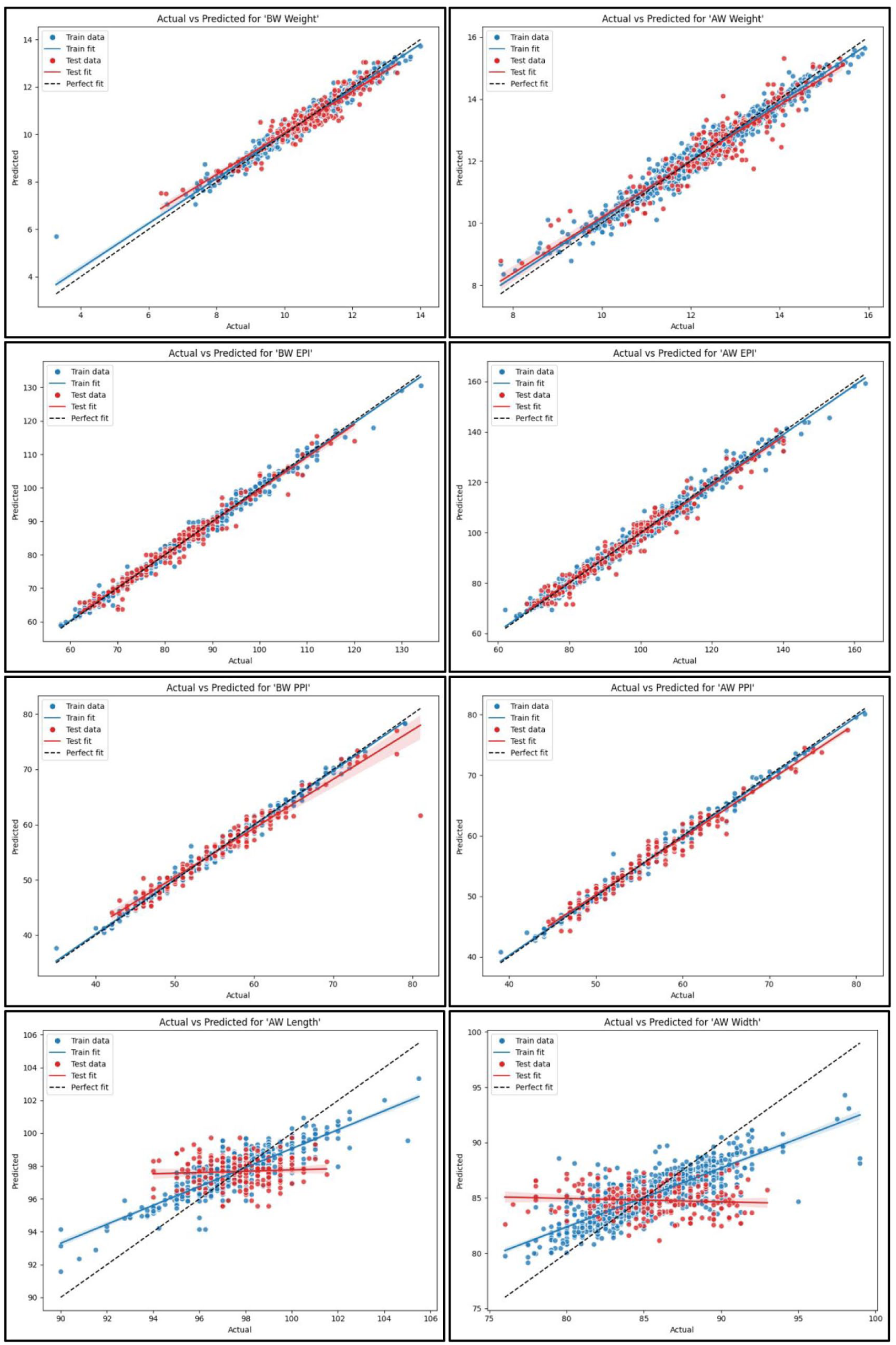
“Actual versus Predicted” plot with train/test data and 95% CIs for the RF model.

In predicting BW Weight, all models performed stably, with multi-way (MW) DOE outperforming one-way DOE, achieving an R² of 0.903, RF at 0.896, and ANN at a slightly higher value of 0.912 among all. MAE values were consistently lower (around 0.3) across all models, whereas MAPE remained close to 2.5%–3.0%. In the case of AW Weight, a similar pattern emerged, with all models delivering strong outcomes. The R² scores spanned from 0.857 (OW DOE) to 0.914 (ANN), and the MAE values were slightly higher than those for BW Weight. For all models, the MAPE values remained below 3.0%.

Thread density-related outputs, that is, BW or AW EPI and PPI, exhibited high predictability with a coefficient of variance higher than 0.93 for all developed models. For BW EPI, R² values exceeded 0.96 across all models, with the ANN model achieving the highest value at 0.979. Meanwhile, MAE and MAPE values ranged from 1.22 to 1.51 and 1.46 to 1.85, respectively. Similarly, in terms of predicting AW EPI, it achieved R² values of 0.949–0.961 across all models. Furthermore, both error metrics remained below 2.5% in all cases, further establishing the predictive stability of the models. All the models performed better for PPIs than EPIs.

These results are reflected in Figure 11, where the three models are compared. The multi-way DOE remained close or even outperformed either RF or ANN or both, in terms of coefficient of variance for specific targets, while achieving excellent values for error matrices. This demonstrates that structured statistical designs continue to hold substantial value in conjunction with machine learning techniques.

The accuracy of these predictions is further confirmed by Figure 12, which shows minimal deviation and tightly bound 95% confidence intervals for all outputs except AW Length and Width.

All models struggled with these two targets, as evidenced by significantly lower R² values, even negative in the case of ANN and RF, indicating a poor model fit. Despite this fact, both MAE and MAPE values remained low, which could falsely imply good performance. The root cause of these poor results is that the dataset used for these two targets was relatively small, while the range of actual values was broad, that is, 94–101.5 cm for AW Length and 76.0–93.0 cm for AW Width in the training dataset, and the testing set spans even wider. In industrial practice, shrinkage values fluctuate within a wide range rather than exact values. This imbalance between data volume and variability in output weakened the model’s ability to predict well, regardless of the method used. Figure 12 visualizes this issue, validates that the dataset was so scattered that the model could not even predict values close to the mean, and underscores the need for larger, more balanced datasets for accurate modeling of dimensional properties.

K-fold cross-validation

Both 5fold and 10-fold validation methods were employed to examine how well the machine learning-based models performed in predicting different fabric properties. Since similar results were obtained for both schemes, only the results of the 5-fold CV are reported. Tables 5 and 6 present the average values and associated standard deviations (±σ) for R², MAE, and MAPE across all targets, with model-wise insights discussed for both RF and ANN, respectively. From the tables, it is observed that the ANN model outperforms the RF model for each output factor; however, it still provides poor results for the last two targets, that is, AW Length and Width, further validating that the dataset was too small for these targets.

Table 5.

Summary of 5-fold cross-validation for the RF model.

Target	R² ± σ	MAE ± σ	MAPE ± σ	Interpretation
BW weight	0.853 ± 0.04	0.32 ± 0.04	3.19 ± 0.65	Good predictive behavior and stable across folds; on average ~ 0.32 oz/yd² off (~3.2% error).
BW EPI	0.954 ± 0.01	1.66 ± 0.18	2.04 ± 0.18	Excellent and consistent; explains >95% of variance with ~1.7 threads/inch error (~2%).
BW PPI	0.948 ± 0.02	0.94 ± 0.11	1.71 ± 0.17	Similarly strong as EPI, with under one pick/inch average error (~1.7 %).
AW weight	0.776 ± 0.04	0.43 ± 0.03	3.58 ± 0.30	Moderately fit; ~78% of variance explained with on average ~ 0.43 oz/yd² off (~3.6% error).
AW EPI	0.934 ± 0.01	2.87 ± 0.29	3.07 ± 0.25	Very good; explains >93% of variance with ~3 threads/inch error (~3.1%).
AW PPI	0.956 ± 0.01	0.88 ± 0.06	1.57 ± 0.13	Excellent and stable; explains >95% of variance with under one pick/inch error (~1.6%).
AW length	−0.335 ± 0.15	1.40 ± 0.15	1.43 ± 0.15	Negative R² indicates performance worse than a constant-mean predictor; though it shows low absolute errors (~1.4 units).
AW width	−0.378 ± 0.10	2.94 ± 0.15	3.45 ± 0.16	Negative R² again; average error (~2.8 units); It validates that the dataset is too low for these targets.

Table 6.

Summary of 5-fold cross-validation for the ANN model.

Target	R² ± σ	MAE ± σ	MAPE ± σ	Interpretation
BW weight	0.899 ± 0.02	0.26 ± 0.01	2.60 ± 0.20	Strong and consistent performance; on average only ~0.26 g off (~2.6% error) across all folds.
BW EPI	0.969 ± 0.00	1.33 ± 0.06	1.62 ± 0.06	Outstanding fit (>96% variance explained) with very low thread-density error (~1.3 threads/inch).
BW PPI	0.958 ± 0.01	0.85 ± 0.07	1.57 ± 0.11	Excellent and stable; the model predicts picks/inch within ~0.85 picks (~1.6%) on average.
AW weight	0.874 ± 0.02	0.33 ± 0.01	2.79 ± 0.08	Very good predictive power after finishing, reducing error to ~0.33 g (~2.8%), a clear improvement over RF.
AW EPI	0.955 ± 0.01	2.28 ± 0.08	2.39 ± 0.06	Highly accurate: explains >95% of variance with ~2.3 threads/inch error (~2.4%).
AW PPI	0.964 ± 0.01	0.78 ± 0.04	1.41 ± 0.07	Superior stability and precision, under one pick/inch error (~1.4%) across folds.
AW length	−0.147 ± 0.07	1.32 ± 0.08	1.35 ± 0.08	R² remains negative, though it’s better than RF, it indicates the ANN still underperforms the mean predictor for fabric length.
AW width	−0.053 ± 0.02	2.58 ± 0.16	3.03 ± 0.18	A near-zero R² indicates marginal improvement, yet it’s a poor result. An increase in the dataset records could improve the results.

Reverse calculation

The study aims to demonstrate that, regardless of the methods used, the textile manufacturing industry can utilize production data to predict target variables by selecting known or required inputs and eliminating traditional trial-and-error methods, such as repeatedly creating sample fabrics to achieve specific required parameters, which wastes both resources and time. Referring to this fact, in this segment, reverse calculations are performed. Thus, the parameters of the required fabric are provided or found from the given sample by the buyer. Now, as a product developer, one should select two crucial parameters, Gray EPI and Gray PPI, to create the gray fabric, which will undergo further processing and ultimately meet the exact requirements requested by the buyer. Moreover, this could be predicted using the existing dataset in the industry and prediction models.

Table 7 presents the performance metrics for both ANN and RF models (the same ones used for forward calculation) in terms of predicting Gray EPI and Gray PPI. At the same time, the input factors included Warp (Ne), Weft (Ne), Spandex (D), Color code, and pre-wash parameters: BW Weight, BW EPI, and BW PPI. Furthermore, Table 8 Shows the same, but in this case, after-wash parameters — that is, AW Weight, AW EPI, and AW PPI — were used as input factors in place of the before-wash parameters, while the other input factors remained unchanged.

Table 7.

Performance metrics that included before-wash parameters as input.

Output	R ²		MAE		MAPE (%)
Output	RF	ANN	RF	ANN	RF	ANN
Gray EPI	0.911	0.914	1.53	1.65	2.30	2.47
Gray PPI	0.966	0.942	0.78	0.81	1.58	1.63

Table 8.

Performance metrics that included after-wash parameters as inputs.

Output	R ²		MAE		MAPE (%)
Output	RF	ANN	RF	ANN	RF	ANN
Gray EPI	0.872	0.871	1.94	2.09	2.97	3.21
Gray PPI	0.972	0.977	0.67	0.68	1.32	1.39

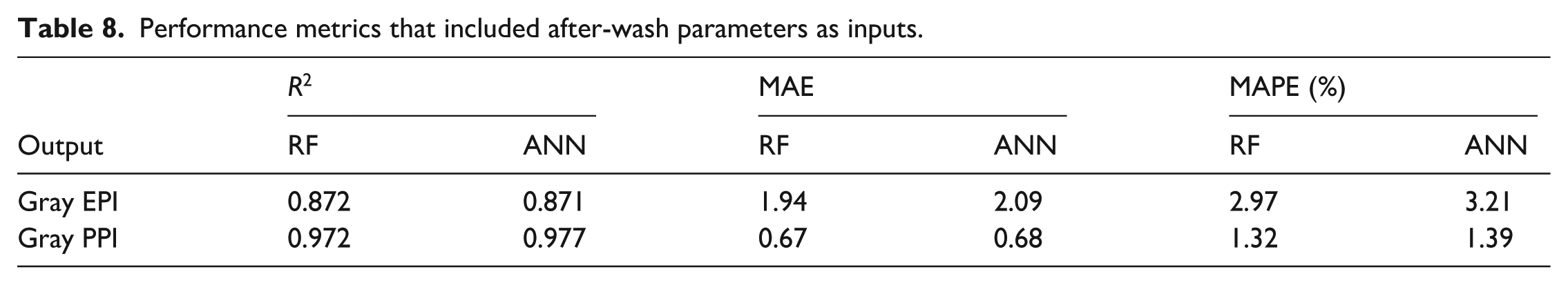
Improved results were obtained in predicting Gray EPI when before-wash parameters were used as inputs rather than after-wash ones. In contrast, for Gray PPI, an opposite manner can be observed. Regardless of the machine learning model type, the performance metrics were excellent, with a high coefficient of variation and low absolute error values (Tables 7 and 8). As a result, it supports the intended outcomes of this research work.

User interface (UI)

To narrow the gap between prediction model development and real-world manufacturing applications, the study developed two interactive user interfaces: a forward prediction user interface driven by an Artificial Neural Network model and a reverse user interface driven by a Random Forest model. The interfaces were designed to demonstrate how manufacturers can leverage data-driven tools in their production processes.

The interface for forward prediction (Figure 13) receives six main production variables from the user: warp count, weft count, spandex count, gray EPI, gray PPI, and color code. Upon clicking the “Predict Properties,” the UI receives the inputs. In the background an ANN model processes these inputs while training itself using 85% of the stored dataset and returns the predicted outputs (e.g. BW/AW Weight, EPI, PPI, Length, Width) along with the expected model accuracy measured as 100% – MAPE, calculated via the remaining 15% of test data. This interface is seamless and operates online, with calculations for the model and error evaluation performed in the background each time a new input is provided.

Figure 13.

User interface for forward way prediction.

Moreover, the inclusion of a reverse prediction model (Figure 14) offers another real-world aspect. For these scenarios, the buyer specifies the end-fabric (before wash or after wash) specification needed, and the developer can utilize the reverse UI to forecast the inputs of gray EPI and PPI. This function is crucial for ensuring that the initial construction of the fabric will ultimately achieve the specified performance upon processing. Thus, the production will be closer to the customer’s specifications from the beginning.

Figure 14.

User interface for reserve way prediction.

What makes the system more useful is flexibility. Regardless of whether the model used in the background is an ANN or an RF one, both are trained on online-stored datasets, the volume of which can be increased by continuously inserting new records, thereby improving the prediction accuracy of the models over time.

Regarding product development, from an industry perspective, employing the interface can significantly minimize dependence on physical sampling, which often demands substantial energy, time, and raw material consumption. Conventionally, identifying a specific set of fabric properties (e.g. GSM, shrinkage) would involve setting up several batches of trial production and adjusting the process parameters iteratively. This not only slows down the product development cycle but also wastes materials and resources.

The sophisticated UI, by contrast, enabled designers, developers, and engineers to model how input choices would affect the results of fabrics without requiring the production of a single sample. This has considerable worth when producing denim, where differential changes in parameters exhibit dramatic effects.

Together, these results also highlight the promise of statistical or machine learning not only as an academic tool but also as an industry solution in modern textile production. The practice can lead to the employment of more data-based, less costly, and environmentally conscious product development across the textile manufacturing industry.

Conclusion

This research work thoroughly examines the use of predictive methods to estimate denim fabric parameters using statistical and machine learning approaches, specifically employing a structured experimental design, decision tree algorithms, and multi-layer neural networks as predictors. The primary objective was to establish a framework that offers reliable prediction and reduces dependency on traditional trial-and-error methods in denim manufacturing, thereby significantly streamlining product development processes.

The results demonstrated high accuracy in predicting critical fabric properties such as weight and thread densities (EPI, PPI), both before and after washing. ANN consistently exhibited superior performance across these parameters, achieving the best R² scores and lowest error metrics (MAE, MAPE). For instance, ANN achieved an R² of 0.912 and 0.914 for before-wash (BW) and after-wash (AW) weights, respectively. Similarly, both statistical (DOE) and RF models exhibited robust predictive capabilities, with multi-way DOE closely matching or surpassing RF in several cases, affirming the continued relevance of structured statistical approaches alongside advanced machine learning techniques.

However, the study revealed notable limitations in predicting dimensional properties, specifically AW length, and width, as all models exhibited significantly lower predictive accuracy (negative R² values). This was attributed primarily to the limited and highly variable dataset available for these particular outputs, underscoring the necessity of larger and more balanced datasets to enhance prediction accuracy for dimensional characteristics.

From an industrial perspective, the development of interactive user interfaces stands out. These tools enable manufacturers to estimate denim characteristics without physical trials, thereby improving decision-making speed and material efficiency. This advancement supports efficient resource utilization and accelerated product development cycles, thereby enhancing overall industry sustainability.

Looking forward, future studies should prioritize enlarging and diversifying the dataset, particularly for dimensional properties, to strengthen predictive model accuracy. Additionally, exploring hyperparameter tuning and advanced deep-learning models could further refine prediction capabilities. Lastly, investigating the integration of these predictive tools into broader automated manufacturing systems represents a promising direction for practical adoption in the industry.

Footnotes

Appendix

Figure 15 and 17 shows Pareto charts and residual plots for one-way regression and multi-way regression of Design of Experiment (DOE), respectively, while Figure 16 Demonstrates feature importances using the Random Forest (RF) model across all output factors (forward approach).

Acknowledgements

The authors would like to express their sincere gratitude to Sister Denims Ltd., a renowned denim manufacturer in Bangladesh, for providing the comprehensive dataset used in this research. Their support in data sharing was essential to the development of predictive models.

Author contributions

Saidul Islam: Conceptualization, Data curation, Methodology, Coding and Software, Investigation, Visualization, Analysis and validation of results, Writing– original draft, Writing– review & editing. Md. Redowanur Rahman: Conceptualization, Literature review, Data collection and curation, Resources, Methodology, Investigation, Analysis and validation of results, Writing– original draft, Writing– review & editing, Project administration. A. T. M. Faiz Ahmed: Conceptualization, Writing– review & editing, Supervision.

Declaration of conflicting interests

The authors declared no potential conflicts of interest with respect to the research, authorship, and/or publication of this article.

Funding

The authors received no financial support for the research, authorship, and/or publication of this article.

ORCID iDs

Saidul Islam

Md. Redowanur Rahman

A. T. M. Faiz Ahmed

Data availability statement

The datasets used and/or analyzed during this study are available from the corresponding author on reasonable request.*

Code availability statement

The codes generated during this study are available from the corresponding author upon reasonable request.*

References

Paul

(ed.) Denim and jeans: An overview. In: Denim: manufacture, finishing and applications. Woodhead Publishing, 2015, pp.1–11. https://doi.org/10.1016/B978-0-85709-843-6.00001-9

Choudhary

Bansal

Influences of elastane content, aesthetic finishes and fabric weight on mechanical and comfort properties of denim fabrics. J Text Eng Fash Technol 2018; 4: 36-42. https://doi.org/10.15406/jteft.2018.04.00119

Periyasamy

Periyasami

Critical review on sustainability in denim: a step toward sustainable production and consumption of denim. ACS Omega 2023; 8: 4472–4490. https://doi.org/10.1021/acsomega.2c06374

Hasan

Asif

Razzaque

, et al. An experimental investigation of different washing processes on various properties of stretch denim fabric. J Mater Sci Chem Eng 2021; 09: 1–15. https://doi.org/10.4236/msce.2021.91001

Salma

Evolution & future of denim trends, market dynamics, and sustainability. Textile Today, 17 May 2025. https://www.textiletoday.com.bd/evolution-future-of-denim-trends-market-dynamics-and-sustainability

Annapoorani

SG.

Introduction to denim. In: Muthu

(ed.) Sustainability in denim. Woodhead Publishing, 2017, pp.1–26. https://doi.org/10.1016/B978-0-08-102043-2.00001-0

Ribeiro

Pilastri

Moura

, et al. A data-driven intelligent decision support system that combines predictive and prescriptive analytics for the design of new textile fabrics. Neural Comput Appl 2023; 35: 17375–17395. https://doi.org/10.1007/s00521-023-08596-9

Studd

The textile design process. Des J 2002; 5: 35–49. https://doi.org/10.2752/146069202790718567

Katırcıoğlu

Aydoğan

Delice

, et al. Predicting quality parameters of denim fabrics using developed ANN based artificial bee colony algorithm. J Text Inst 2024; 115: 757–767. https://doi.org/10.1080/00405000.2023.2201560

10.

Kazemi

Shafighfard

Yoo

DY.

Data-driven modeling of mechanical properties of fiber-reinforced concrete: a critical review. Arch Comput Methods Eng 2024; 31: 2049–2078. https://doi.org/10.1007/s11831-023-10043-w

11.

Badini

Regondi

Pugliese

Unleashing the power of artificial intelligence in materials design. Materials 2023; 16: 5927. https://doi.org/10.3390/ma16175927

12.

Tran

, et al. Modeling of textile manufacturing processes using intelligent techniques: a review. Int J Adv Manuf Technol 2021; 116: 39–67. https://doi.org/10.1007/s00170-021-07444-1

13.

Chauhan

Yadav

Arya

Application of artificial neural networks in textiles. Int J Curr Microbiol App Sci 2018; 7: 3134-3143. https://doi.org/10.20546/ijcmas.2018.704.356

14.

Chattopadhyay

Guha

Artificial neural networks: applications to textiles. Text Prog 2004; 35: 1–46. https://doi.org/10.1080/00405160408688961

15.

Hui

CLP

Fun

Review of application of artificial neural networks in textiles and clothing industries over last decades. In: Suzuki

(ed.) Artificial neural networks - industrial and control engineering applications. IntechOpen, 2011. https://doi.org/10.5772/16003

16.

Malik

Kocaman

Kaynak

, et al. Analysis and prediction of air permeability of woven barrier fabrics with respect to material, fabric construction and process parameters. Fibers Polym 2017; 18: 2005–2017. https://doi.org/10.1007/s12221-017-7241-5

17.

Zulfiqar

Manzoor

Ijaz

, et al. Artificial-neural-network-based predicted model for seam strength of five-pocket denim jeans: a review. Textile 2024; 4: 183–217. https://doi.org/10.3390/textiles4020012

18.

Bilisik

Demiryurek

Analysis and tensile-tear properties of abraded denim fabrics depending on pattern relations using statistical and artificial neural network models. Fibers Polym 2011; 12: 422–430. https://doi.org/10.1007/s12221-011-0422-8

19.

Zeydan

Prediction of fabric tensile strength by modelling the woven fabric. In: Dubrovski

(ed.) Woven fabric engineering. IntechOpen, 2010. https://doi.org/10.5772/10473

20.

Kularatne

SDMW

Ranawaka

RAHS

Fernando

EASK

, et al. Machine learning-based approach for modelling elastic modulus of woven fabrics. In: Moratuwa engineering research conference (MERCon), 2020, pp. 470-475. https://doi.org/10.1109/MERCon50084.2020.9185295

21.

Kastaci

Özek

Özhan

A comparison of the three different techniques in predicting breaking strength of cotton and blended woven fabrics. Tekstil ve Muhendis 2024; 31: 34–41. https://doi.org/10.7216/TEKSMUH.1329122

22.

Seçkin

AÇ

Demircioglu

, et al. FabricNET: a microscopic image dataset of woven fabrics for predicting texture and weaving parameters through machine learning. Sustainability 2023; 15: 15197. https://doi.org/10.3390/su152115197

23.

Antony

(ed.) Fractional factorial designs. In: Design of experiments for engineers and scientists. 2nd Ed. Elsevier 2014, pp. 87-112. https://doi.org/10.1016/b978-0-08-099417-8.00007-9

24.

Brook

Arnold

GC.

Applied regression analysis and experimental design. CRC Press, 2018. https://doi.org/10.1201/9781315137674

25.

Çubukçu

HC.

Performance evaluation of internal quality control rules, EWMA, CUSUM, and the novel machine learning model. Turk J Biochem 2021; 46: 661–670. https://doi.org/10.1515/TJB-2021-0199

26.

Antony

(ed.) Fundamentals of design of experiments. In: Design of experiments for engineers and scientists. Elsevier, 2023, pp. 7-18. https://doi.org/10.1016/b978-0-443-15173-6.00010-x

27.

Breiman

Random forests. Mach Learn 2001; 45: 5-32. https://doi.org/10.1023/A:1010933404324

28.

Hastie

Tibshirani

Friedman

(eds) Random forests. In: The elements of statistical learning. 2nd ed. Springer, 2009, pp.587-604. https://doi.org/10.1007/978-0-387-84858-7_15

29.

Pedregosa

Varoquaux

Gramfort

, et al. Scikit-learn: machine learning in python. J Mach Learn Res 2011; 12: 2825-2830.

30.

Sukpancharoen

Wijakmatee

Katongtung

, et al. Data-driven prediction of electrospun nanofiber diameter using machine learning: a comprehensive study and web-based tool development. Res Eng 2024; 24: 102826. https://doi.org/10.1016/j.rineng.2024.102826

Prediction of fabric properties of denim fabrics using statistical and machine learning methods

Abstract

Keywords

Introduction

Materials and methods

Materials

Fabrication process

Data collection & sorting

Development of a workable dataset

Input and output parameters

Charts for effect analysis

Prediction models

Design of experiments (DOE)

Random forest (RF)

Artificial neural network (ANN)

K-fold cross-validation

Performance metrics

Reverse calculations

Development of user interface (UI)

Results and discussion

Significance of input variables on the fabric properties

Prediction performance of different models

K-fold cross-validation

Reverse calculation

User interface (UI)

Conclusion

Footnotes

Appendix

Acknowledgements

Author contributions

Declaration of conflicting interests

Funding

ORCID iDs

Data availability statement

Code availability statement

References