Sage Journals: Discover world-class research

Abstract

Using quadratic B-spline curves to generate 3D fiber paths, this study proposes a novel approach to fiber-level modeling based on the matrix transformation framework. This framework ensures a unified form and explicit rules, enabling convenient, flexible and efficient operations with excellent computability and parameter scalability. The braided yarn configuration is accurately described by an innovatively introduced fiber distribution function accounting for fiber count, internal or external transfer and distribution in the cross-section of bundle. Adding twisting parameters such as twisting degree, twist angle and twist direction significantly improves the texture and 3D visualization effect of twisted braided yarn. Net-shaped or curved tubular fiber-level braided structures are flexibly modeled using tape and strand units. Parameter optimization enhances computational efficiency and geometric adaptability. The simulation results demonstrate that the framework enable accurate simulation of various braided configurations and achieve fully parameteric modeling and flexible changes of 2D circular braided fabrics, producing geometric models with excellent structural continuity, suitable for fiber-scale mechanical analysis and providing an effective architectural support for digital modeling and multi-scale performance prediction of braided composites.

Keywords

2D circular braided fabrics fiber-level modeling parameters simulation models fabric simulation

Introduction

Braided structures are created by interlacing yarns in clockwise and anticlockwise directions in order to form a bias structure along the longitudinal axis. A powerful and complex tool designed especially for modeling and analyzing fiber-level braided structures has been developed as a result of advancements in computer hardware technology. This advanced tool synergizes the finite element method with computer-aided design, allowing for an in-depth analysis of the interactions between fibers, the distribution of stresses and displacements within these fiber-level braided structures.^1
–3 A precise and accurate simulation model is the necessity and foundation of this analytical approach. Scholars have developed static models and provided pertinent mathematical equations for the long-term development of fabric simulation technologies.^4,5 However, fiber-level modeling still has issues like laborious modeling procedures, low fault tolerance, poor computational efficiency, limited parameter control capabilities and subpar simulation results due to the yarn’s complex structure and highly nonlinear braided topology.⁶

Currently, in the modeling and 3D simulation of fiber-level fabrics, Huang et al.^7,8 devised a method to reconstruct the geometry of 2D multilayer textiles from low-resolution CT scans. The digital material twins created in this way helped researchers predict the mechanical characteristics of braided fabrics, such as failure and damage, by exposing the geometric structure of 2D multilayer fabric layers and characterizing the morphological aspects of fibers. Nevertheless, the extensive use of CT-based modeling techniques in fiber recognition, path tracking, and image segmentation was severely limited by the need for extensive image preprocessing, which was costly, time-consuming, and difficult to implement. Ghaedsharaf et al.^9,10 modeled a biaxial braided preform based on fiber-level numerical simulations. Using virtual truss unit fibers, the model produced the perfect loosely braided geometry. To get realistic braided geometry, tiny loads were added to the original fiber structure. However, when handling complex geometries and material behaviors, the fiber-level numerical simulation demanded a significant amount of processing resources, which restricted the model’s application. Kyosev^11,12 developed Texmind Braider, which integrates yarn configuration, color design, and 3D visualization functions, employing a braiding process-based generalized topological model to enhance the design of tubular and flat braided fabrics. However, its modeling was limited by yarn axis curvature fluctuations that impaired normal vector definition and visualization, and by polynomial interpolation that may cause topological errors in multifilament simulations, hindering structural simulation accuracy. Depending on the different twisting conditions, fibers in the fabric structure significantly exhibit different yarn morphologies and mechanical properties. Zheng and Huang¹³ used B-spline curves for 1D and 2D texture to simulate the twisting effect, but the enlarged image of the twisted yarn from 1D twisting did not meet design requirements, and the 2D twist mapping technique required excessive storage for texture image files. Xu and Qian¹⁴ developed a model to predict how twisted yarn affects the stiffness of four-directional braided composites, calculating yarn elastic properties by introducing average twist. They used MCM theory and stiffness-volume averaging to assess each cell’s contribution to the overall elastic properties, but they did not take into account the impact of different twist sizes on stiffness in the modeling.

This paper explores a fiber-level modeling for 2D circular braided structures using matrix transformation framework for the first time. This approach avoids the normal vector distortion and topological errors caused by severe curvature fluctuations and polynomial interpolation, directly constructing spatial fiber trajectories through analytical matrix operations, in contrast to the application of Kyosev’s generalized topological models in TexMind Braider.^11,12 This provides a new theoretical tool for multi-scale simulation and real-time design optimization. The method begins by taking into account the quantity of cross-sectional fibers, the internal and external transfer of fibers, the distribution of fiber in order to develop the fiber distribution function. A model of twisted strand incorporating twisting degree, twist angle and twist direction enhances texture simulation effect. The matrix transformation framework enables simulation of 2D circular braids and flexible extension to curved tubular or net-shaped braids, ensuring high universality and parametric adjustment. The 3D simulation process is realized through Visual Studio 2019.

Morphological characteristics and structure of 2D circular fiber-level braided fabrics

Morphological characteristics

The thickness of the 2D circular fiber-level braided fabric does not exceed three times the diameter of the braided yarns. Less fiber mechanical damage and simple process, design flexibility, near-net size forming can be used as a variety of pipes, pipe shells, bushings, ultra-high-temperature insulation pipe and a variety of structural support for the reinforcements of the composite material.¹⁵ Because of their exceptional impact resistance, lightweight design, and other features, these items are widely used in a variety of industries, including aerospace, defense, transportation, and construction. The fiber-level braided structure appropriately adapts to the braided structure’s properties while also taking into account the fibers’ specifics, such as their cross-section, radial specifications, and spatial correlations.^16,17

The braided structures can typically be classified into three primary forms: diamond (1:1), regular (2:2), and hercules (3:3) braids. In a diamond braid, each yarn crosses above and below the other yarn in a repeating manner.^18
–20 The simulations in this paper are based on a 2D circular braided fabric with regular braided structure as an example (the braided fabric has 12 braided yarns, each with 6 fibers) to construct a fiber-level mathematical structure model and carry out a 3D simulation.

Formation of braided structures

A standard braiding machine consists of several necessary components, such as a mandrel, yarn carriers, a braiding ring and a braiding plane, as illustrated in Figure 1. Two sets of yarn carriers travel the generalized rose curve on the braiding plane. One set rotates in the clockwise direction, the other operates counter-clockwise. These carriers interlace with each other to form a braided structure on the mandrel during the braiding process. Finally, the take-up rollers move the mandrel at a predetermined speed to complete the continuous braiding.^21,22

Figure 1.

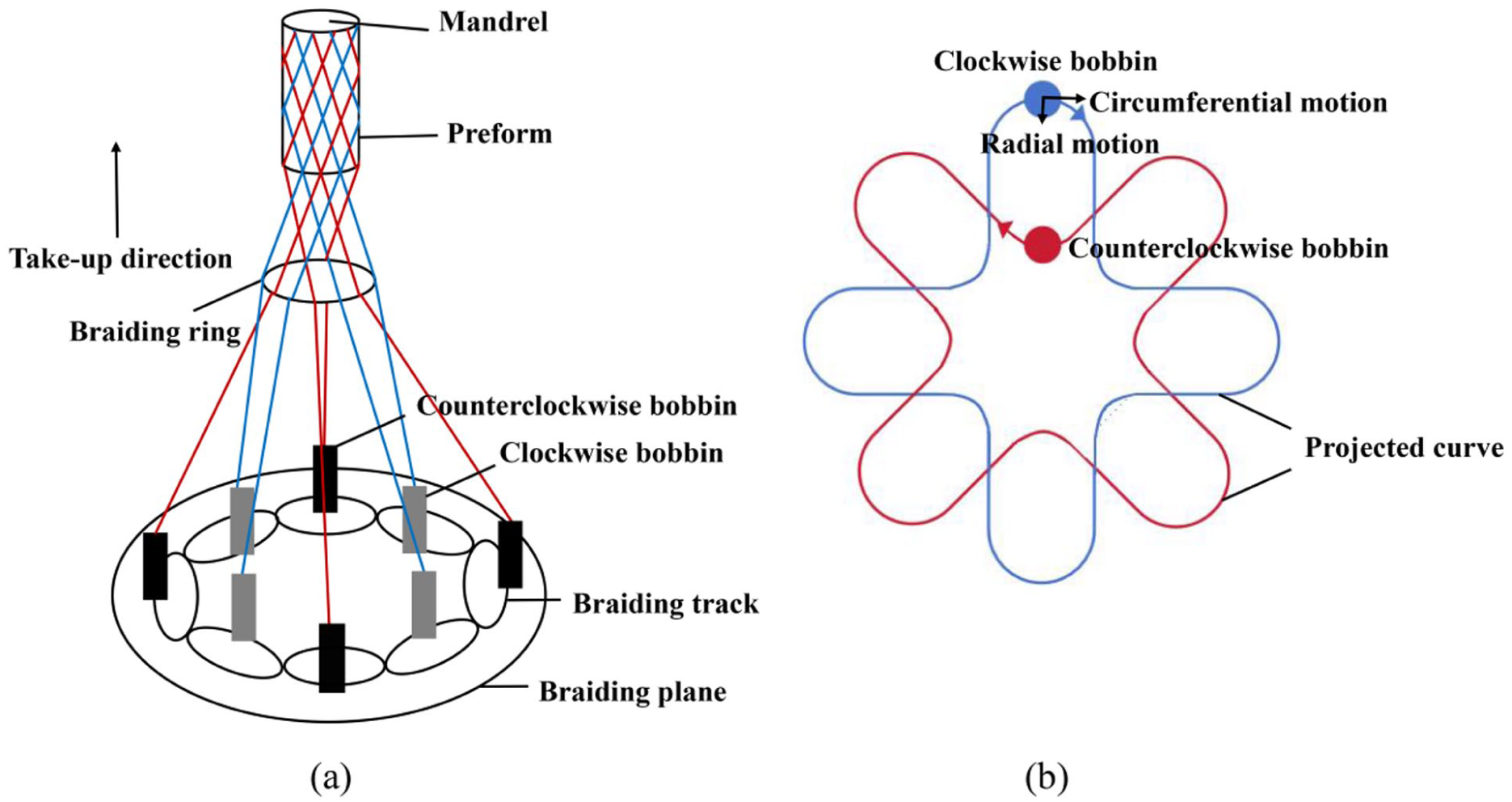
Two-dimensional circular braiding process. (a) A schematic representation of braiding. (b) Yarn carrier trajectory.

Geometrical modeling of 2D circular fiber-level braided structures

Assumptions

(1) Adjacent fibers do not intersect or penetrate each other. They are in close proximity and treated as incompressible.

(2) Fibers in the same direction have the same braiding pattern, differing only in initial position.

(3) The fibers possess a circular cross-section characterized by radius r.

(4) The braid is a 2D circular braided fabric with regular braided structure.

Generation of braided structures

Definition of geometric parameters

In order to derive the equation of fiber-level braided curve, the following parameters concerning the braided structure are defined.

(1) Radius of fiber (r). The radius of a fiber is associated with the diameter of a single fiber and an increase in radius of fiber typically indicates an improved load-bearing capability.

(2) Fiber distribution (f_(k)). The fiber distribution describes the specific location of each fiber in a strand of fiber bundle.

(3) Number of fibers in the bundle (d). It refers to the total number of single fibers that come together to form a unified entity, which directly influences the tensile strength, flexibility and overall performance of the fiber bundle.

(4) Total Number of Braided Yarns (n): This metric denotes to quantify the total number of braided yarns employed in the braided structure. Generally, greater strength and longevity of the fabric are correlated with more braided yarns.^23,24

(5) Degree of Twisting (A): This parameter measures the extent of twisting in the yarns and is related to the twisting pitch. It affects the strength and flexibility of the yarn. A stronger and more rigid yarn might be produced with a higher degree of twisting.¹⁸

(6) Numbering of braided yarn (i). The numbering of braided yarn specifies the order in which braided yarns are to be braided.²⁵

(7) Amplitude of braided yarn (a). The amplitude of braided yarn refers to the amplitude or offset of a yarn in a particular direction in a braided structure. By adjusting the parameter, it affects the texture and appearance of the fabric for design purposes.^26,27

(8) Radius of braided fabric (R). R is defined as the distance from the braiding axis to the central circle which the crimps wave around.

(9) Numbering of points on a single fiber (j). It refers to the numbering of points scattered in sequence within a single fiber. A more precise morphological structure of the fiber is often implied by a larger number of spots.^28,29

(10) Radius of twisted strand (R_y). The radius of twisted strand describes the cross-sectional dimensions of twisted strand, calculated by the distance from the center of yarn C_y to the center of fiber C_f.

(11) Angle of twist (β_twist). It refers to the angular displacement that a single fiber experiences within a strand relative to its longitudinal axis.

(12) Angle between fibers (θ_d). The angle between the centers C_f of two fibers in the same fiber bundle relative to the center C_y of the yarn.

(13) Braiding angle (α). It is the angle between the tangent to the yarn path and the axial direction of the braid.

(14) Inter-yarn gap (f). It is the surface-to-surface distance between adjacent yarns from different yarn groups.

(15) Inter-yarn spacing (c). It refers to center-to-center distance between adjacent yarns from different yarn groups.

(16) Floating length (p). It refers to the distance a yarn travels between many interlacing locations on the outside or inside of a fabric without interlacing with the opposing yarn system.

(17) Total number of yarns in a group (Q): It refers to the total number of yarns per group in the braided structure.

(18) Numbering of yarn in a group (q). It refers the numbering sequence of yarns in each group of the braided structure.

(19) Proportionality coefficient (b). It changes the point distribution density of each fiber along the z-axis direction to accurately capture its morphology.

(20) Translation distance along the x-axis (S).

(21) Translation distance along the z-axis (Z).

(22) Equation of a single fiber (L₀ )

Construction of fiber distribution function

(1) As shown in Figure 2, the linear equation (vectorial) of a single fiber is established in matrix form. And equation (1) is used to describe and store the coordinates of points (0,0,bj) on a single fiber. The numbering of points on the single fiber is represented by the parameter j, an integer loop variable that iterates from 0 to the total number of points on the fiber. π is the PI and has a value around 3.14159. Dense point counting refines the description of the morphology of a single fiber. The point distribution density of a single fiber along the z-axis direction is determined by parameter b, which serves as a proportionality coefficient to regulate the density of discrete points on the fiber. The parametric equation L₀ represents the 3D coordinates of a series of points uniformly distributed on a single fiber to be simulated.

(2) A single fiber is represented by equation (1) in the preceding step. To determine the position of a fiber that makes up a fiber bundle, shift the single fiber outside of the z-axis using the translation matrix T₁ shown in equation (2). The points on the new single fiber equation L₁ may be obtained by applying equation (3) to translate the single fiber equation L₀ by 2r in the direction of the x-axis. Figure 2(a) and (b) depict the changes of a single fiber.

L_{0} = {[0, 0, b j, 0]}^{T}

(1)

T_{1} = [\begin{array}{l} \begin{matrix} 1 & 0 & 0 & 2 r \end{matrix} \\ \begin{matrix} 0 & 1 & 0 & 0 \end{matrix} \\ \begin{matrix} 0 & 0 & 1 & 0 \end{matrix} \\ \begin{matrix} 0 & 0 & 0 & 1 \end{matrix} \end{array}]

(2)

L_{1} = T_{1} \cdot L_{0}

(3)

(3) Many fibers are equally distributed using the rotation matrix R₁ of equation (4) to produce the fiber bundle seen in Figure 2(c). Figure 5(a) displays the cross-section of the fiber bundle. The angle θ_d between fibers in a fiber bundle is defined by the formula θ_d = 2π/d. In a fiber bundle consisting of six fibers, each fiber completes a full rotation around the circumference, resulting in a rotation angle of θ_d for each fiber. Thus, the angle between any two adjacent fibers is ascertained as 2π/6 = π/3. The variable k in equation (4) represents the location of the different fibers and ranges from 0 to 5, meaning that there are 6 different locations for the fibers in Figure 2(c). Thus, the angle of the k^th fiber relative to the initial fiber is πk/3. In equation (4), the point on the equation of single fiber L₁ can be rotated around the z-axis by πk/3 to obtain the point on the k^th fiber, corresponding to the position of the six uniformly distributed fibers.

(4) equation (5) displays the fiber distribution function that was created by analyzing the composition of the fiber bundles in 2D circular fiber-level braided fabrics. This technique allows for accurate modeling of the tubular structure. In a 2D circular braided fabric, the single yarn contains several finely braided fibers. A twist is created by the fiber bundles spiraling up the center of the yarn. When determining the control points of each fiber in the yarn, simulation of tubular geometry can be performed.

R_{1} = [\begin{matrix} \cos (θ_{d} k) & - \sin (θ_{d} k) & 0 & 0 \\ \sin (θ_{d} k) & \cos (θ_{d} k) & 0 & 0 \\ 0 & 0 & 1 & 0 \\ 0 & 0 & 0 & 1 \end{matrix}]

(4)

L_{2} = R_{1} \cdot L_{1}

(5)

Figure 2.

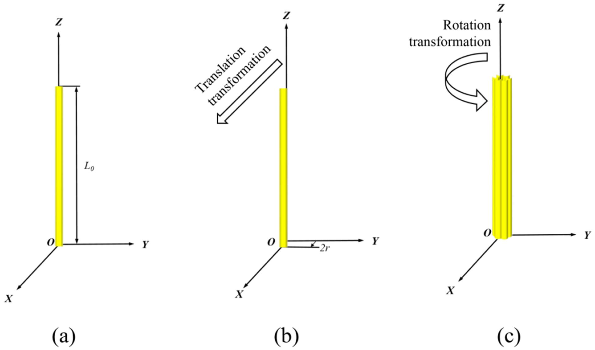
Formation diagram of fiber distribution. (a) Spatial position of a single fiber. (b) Post-translational position of fiber. (c) Morphology of fiber bundle.

Mathematical modeling of strands

(1) The characteristics of the strand are intricately linked to the pitch of the spiral in Figure 3. The change in pitch directly affects the physical properties and application characteristics of the strand. By adjusting the degree of twisting A, the pitch of the spiral can be flexibly adjusted. A variable pitch braided structure can be achieved by adjusting the degree of twisting A and defining the spiral as a variable pitch. This structure provides enhanced mechanical properties and comfort for specific applications.

Figure 3.

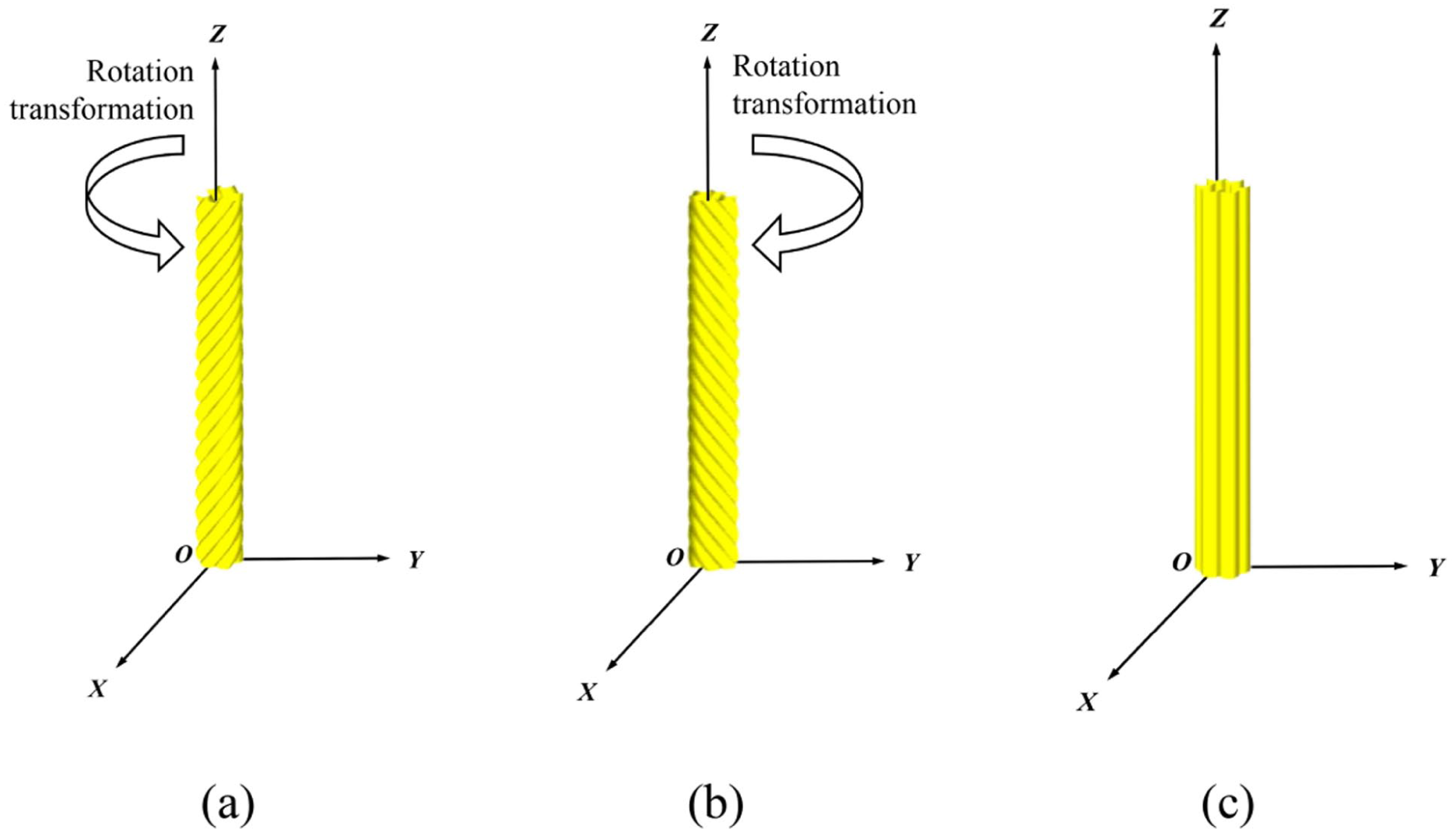
Morphology of strand unit. (a) Z-twist. (b) S-twist. (c) No twist.

As shown in Figure 5(b) for the twisting path of a twisted strand, the center of the yarn C_y to the center of the fiber C_f is calculated as the radius of twisting using equation (6). A_j is the angle of rotation that the twisted strand passes through at each j-value. The value can be used to derive the coordinates of any point on the centerline of each fiber in the twisted strand using this equation.

The radius of the strand R_y is three times than the radius of the fiber. Ideally, the fiber center C_f varies cyclically with the cyclic twisting loops when the fiber strand is twisted cyclically using repetitive twisting loops. The fiber center C_f is rotates around the yarn center C_y once for every twist.

As shown in Figure 3(a) and (b), the fiber bundle is twisted into strands using the rotation matrix R₂ in equation (6). The yarn is obtained by twisting in counter-clockwise (Z-twist) direction and clockwise (S-twist) direction in Figure 4(a) and (b). If A equals 0, the formula (6) can be obtained without twisting the strand in Figure 3(c). In practice, the 2D circular fiber-level braid is characterized by twisted strands with Z-twist in one direction and S-twist in the other direction. This allows the braided rope to be uniformly stressed among the strands. The torque direction of each strand is the same when the twist direction of each strand is the same (all Z-twist or S-twist). The torsion force is superimposed on each other, causing the rope to rotate along the torsion direction to achieve torque balance. This can lead to the braided strands of the rope twisting together in a slack state, potentially affecting normal use and causing damage. During the braiding process of braided ropes, the strands rotate along either counter-clockwise or clockwise trajectories. Each complete rotation adds or removes one twist to the yarn between the bobbin and the braiding point, leading to significant differences in yarn twist for both directions. This variation affects the appearance and inherent properties of the braided rope.

R_{2} = [\begin{matrix} \cos (A j) & {(- 1)}^{i + 1} \sin (A j) & 0 & 0 \\ {(- 1)}^{i} \sin (A j) & \cos (A j) & 0 & 0 \\ 0 & 0 & 1 & 0 \\ 0 & 0 & 0 & 1 \end{matrix}]

(6)

L_{3} = R_{2} \cdot L_{2}

(7)

Figure 4.

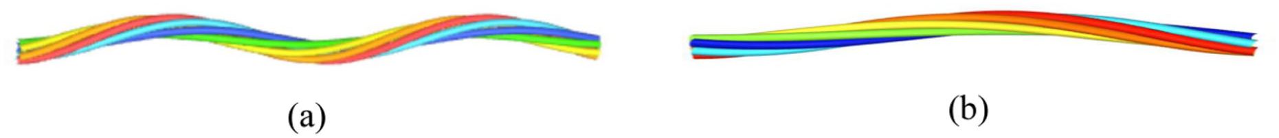
Strands (a) S-twist. (b) Z-twist.

Where: i is the numbering of braided yarn and the value ranges from 0 to n−1. The total number of braided yarn is n. The value of A affects the size of the braiding angle and A takes the value of 1 when twisted and 0 when not twisted in this case.

In Figure 5(a), a cross-section of a fiber bundle is shown when six fibers are used to form a fiber bundle for braiding. Figure 5(b) depicts the twisting route of the fiber bundle. The twist in space is expanded into a plane to form a right-triangle in Figure 5(c). One of the right-angled side length is the circumference of the yarn 2πR_y. And the other right-angled side is the twisting pitch, it is inversely proportional to the degree of twisting. Through the relationship between the degree of twisting A and the yarn radius R_y, the angle of the twistback β_twist can be calculated according to equation (8).

β_{t w i s t} = \arctan (2 π A R_{y})

(8)

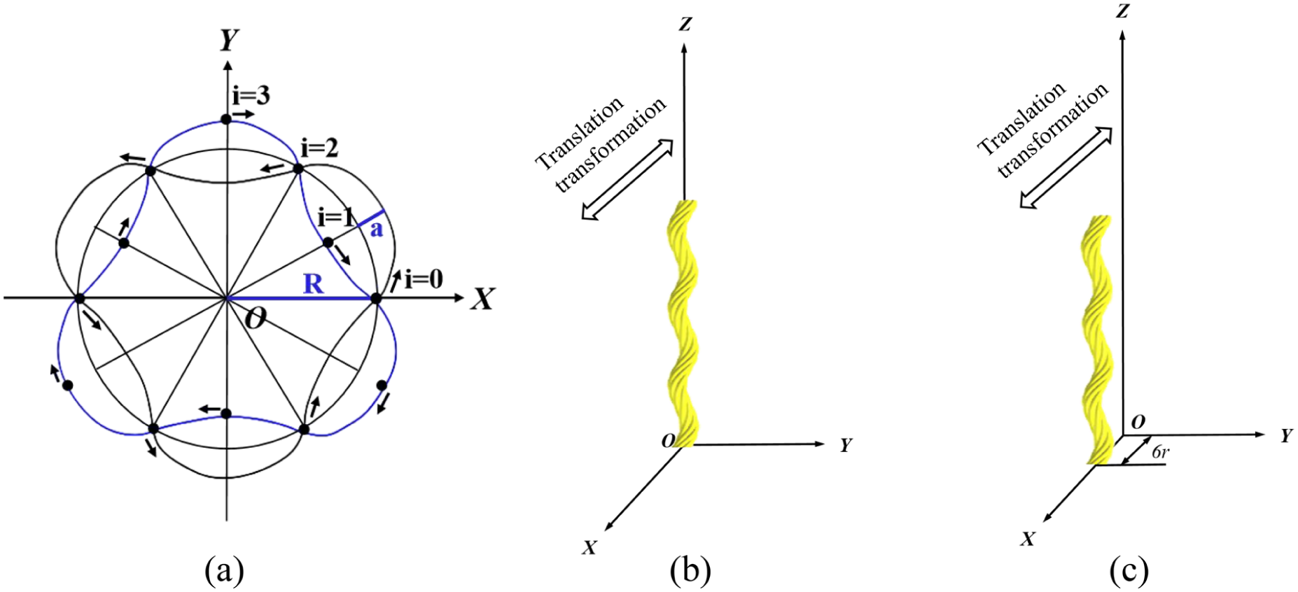
(2) The up-and-down float of a yarn is represented as a sine function to describe how many yarns it spans. As shown in Figure 6(a), the cross-sectional yarn trajectory in a braid with floating length 2 oscillates around a circle of radius R. the fluctuations along the coordinate axis are modeled by a sine function, and each arc inside and outside the circle is defined by four coordinate points. The trajectories of the braided yarns labeled i = 0, 1, 2, and 3 in the regular braided structure are described by distinct mathematical expressions. As i increases, the trajectory formulas repeat cyclically every four yarns. When i = 0, the first yarn’s trajectory rises and then curves downward, represented as asin(πj/4). Similarly, the second, third, and fourth yarns follow asin(πj/4−π/2), asin(πj/4 + π) and asin(πj/4–3π/2), respectively. Applying this approach to diamond and hercules braids reveals that two and six distinct mathematical equations are needed to characterize their cross-sectional yarn trajectories. Equation (9), derived from these mathematical equations, universally describes sinusoidal yarn morphology for varying floating lengths, where p denotes the floating length. For example, p = 2 for regular braid.

Figure 5.

Model of braided yarn. (a) Cross-section of fiber bundle. (b) Twisting process of fiber bundle. (c) Twist angle and twist pitch.

Figure 6.

Regular braided structures. (a) Yarn trajectory in the cross-sectional direction. (b) Sinusoidal braided yarn. (c) Yarn after translation.

The vertical braided yarn becomes a sinusoidal braided yarn with wavy curvature in Figure 6(b). Where: a is the amplitude of the wave, which can take a value equal to the radius of the fiber bundle. In this example, a can take the value of 3r for a bundle of six fibers. Parameter i is the numbering of the braided yarn. 2D circular braided fabrics made of braided yarns interlaced in both clockwise and counter-clockwise directions. The braided surface is obtained by the contour of the braided structure and interlacing rules. The braided surface has similar overall contour. The wave amplitude a is equal to the amplitude of the trigonometric function. This series of wave structures allows the yarns to interlace with each other in both clockwise and counter-clockwise directions without overlapping.

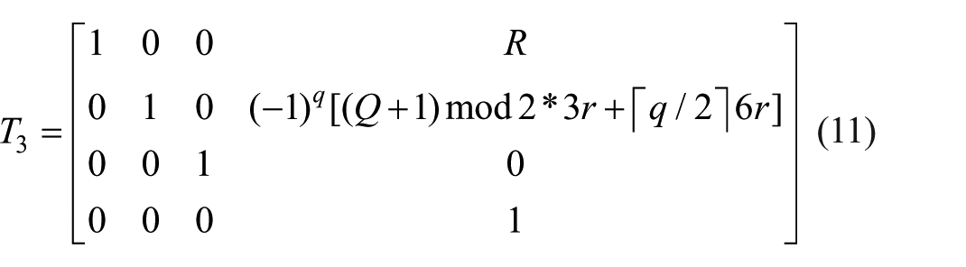
(3) Figure 6(c) illustrates how the trace of strand is translated along the x-axis by a distance R using equations (11) and (12). It will prepare for the subsequent formation of multiple wavy braided yarns from a single wavy braided yarn around the z-axis in the next step, where R is the radius of the 2D circular braided fabrics. In equation (11), R can be taken as R = 6r if the braided rope is braided with 12 braided yarns.

T_{2} = [\begin{array}{l} \begin{matrix} 1 & 0 & 0 & a \sin [π j / 4 + {(- 1)}^{i} (i \mod 2 p) π / p] \end{matrix} \\ \begin{matrix} 0 & 1 & 0 & 0 \end{matrix} \\ \begin{matrix} 0 & 0 & 1 & 0 \end{matrix} \\ \begin{matrix} 0 & 0 & 0 & 1 \end{matrix} \end{array}]

(9)

L_{4} = T_{2} \cdot L_{3}

(10)

To create braid with one yarn in a group, the single yarn must be translated R along the x-axis. The braid with two yarns in a group is created by translating the single yarn R along the x-axis, followed by displacements of ±3r along the y-axis to determine the position of the two yarns in a group without interpenetration. The two yarns in a group are treated as a whole in the subsequent R₃ and R₄ matrix transformations (yarn group generation and interlacing), ensuring proper intra-group filling. Similarly, three transformations are carried out to obtain three yarns in a group based on the translation distance R of a single yarn along the x-axis: keeping the original position, translating by +6r, and translating by −6r along the y-axis. This forms a non-interpenetrating spatial arrangement for a group of three yarns. Subsequently, matrix transformation equation (11) generalizes this configuration to form a group of two or more yarns, using (Q + 1) mod 2 to assign distinct transformations to even or odd numbered yarns in a group. Here, braid with one yarn in a group corresponds to Q = 1 and q = 0.

T_{3} = [\begin{matrix} 1 & 0 & 0 & R \\ 0 & 1 & 0 & {(- 1)}^{q} [(Q + 1) \mod 2 * 3 r + ⌈ q / 2 ⌉ 6 r] \\ 0 & 0 & 1 & 0 \\ 0 & 0 & 0 & 1 \end{matrix}]

(11)

L_{5} = T_{3} \cdot L_{4}

(12)

(4) Applying equations (13) and (14), the positions of all the wavy braided yarns are determined in preparation for the interlacing of odd and even-numbered braided yarns in the next step. By rotating the wavy braided yarns around the z-axis to the braided position, the wavy odd and even-numbered braided yarns in the z-axis direction are obtained in Figure 7. Where: i is the numbering of the braided yarn, which ranges from 0 to n−1. And n is the total number of the braided yarn. The phase difference of the counter-clockwise braiding curves is π/3 when the braided structure is regular structure. So the initial angles of the six counter-clockwise braiding curves are 0, π/3, 2π/3, π, 4π/3 and 5π/3, respectively. The phase difference of clockwise braiding curves is also π/3. There is a phase difference of π/6 in the neighboring braiding curves of different directions. The initial phase differences of the braided curves are π/6, π/2, 5π/6, 7π/6, 3π/2, and 11π/6, respectively.

R_{3} = [\begin{matrix} \cos (2 π i / n) & - \sin (2 π i / n) & 0 & 0 \\ \sin (2 π i / n) & \cos (2 π i / n) & 0 & 0 \\ 0 & 0 & 1 & 0 \\ 0 & 0 & 1 & 0 \end{matrix}]

(13)

L_{6} = R_{3} \cdot L_{5}

(14)

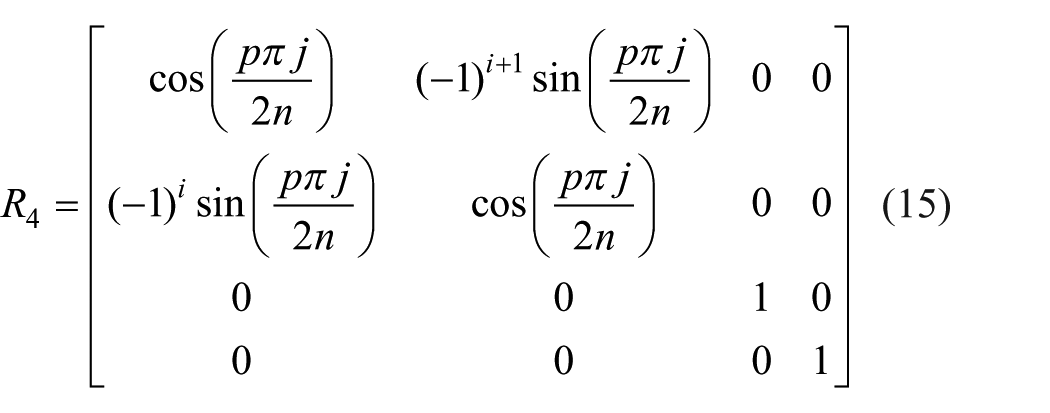
(5) The odd and even-numbered braided strands interlaced with each other to form a braided structure using equations (15) and (16). The odd and even-numbered braided yarns are rotated around the z-axis respectively to form the interlaced pattern in Figure 8(b) and (c). As shown in Figure 8(a), the cross-sectional interlaced pattern of single braided yarns is similar to the three-petal shape. The interlacing transformation of the braided yarns can be accomplished to obtain all the 12 curved braided yarn curves based on these data and the matrix transformations in Figure 8. The modeling of different braided structures is most closely associated to equations (9) and (15). Using equation (9) with a specified amplitude a = 3r and a floating length p = 2, a sinusoidal braided yarn with two yarn spans is produced when it is a regular braid. The interlacing of the resulting sinusoidal braided yarn is modified using equation (15). Make sure that the braided yarns in the same direction will not collide, while those in opposite directions will not interfere with each other. In the analysis of braided structures, n and p are related such that the minimum value of n is 4p. The value of n is discontinuous and it needs to satisfy n/p mod 2 = 0. Figure 9 shows the final geometric structure of the 2D circular fiber-level braided fabric.

R_{4} = [\begin{matrix} \cos (\frac{p π j}{2 n}) & {(- 1)}^{i + 1} \sin (\frac{p π j}{2 n}) & 0 & 0 \\ {(- 1)}^{i} \sin (\frac{p π j}{2 n}) & \cos (\frac{p π j}{2 n}) & 0 & 0 \\ 0 & 0 & 1 & 0 \\ 0 & 0 & 0 & 1 \end{matrix}]

(15)

L_{7} = R_{4} \cdot L_{6}

(16)

(6) In summary, the matrix transformed quadratic B-spline curve may be used to get equation (17) for the fiber profile in braided ropes. The transformation matrix is denoted by M:

L_{1} (i, k) = R_{4} \cdot R_{3} \cdot T_{3} \cdot T_{2} \cdot R_{2} \cdot R_{1} \cdot T_{1} \cdot L_{0} = M \cdot L_{0}

(17)

M = R_{4} \cdot R_{3} \cdot T_{3} \cdot T_{2} \cdot R_{2} \cdot R_{1} \cdot T_{1}

(18)

Figure 7.

Rotational transformation of braided yarns.

Figure 8.

Interlacing transformations of braided yarns. (a) cross-section of braided yarns. (b) counter-clockwise rotation of braided yarns. (c) clockwise rotation of braided yarns.

Figure 9.

2D circular fiber-level braided geometry.

Parameter changes for mathematical modeling

To obtain the fiber profile equations for different braided structures, the parameters in the quadratic B-spline curves based on the matrix transformation are changed as follows.

(1) The distance 2r is variable in equation (2). Chang 2r to br, with b as a variable coefficient. And br determines the radius of the final braided yarn for strand unit and affects the radius of the braid in the strand-unit to form a 2D circular braid with different fiber volume contents and morphologies.

(2) Fibers have different distributions in equation (4). And the fiber distribution is $f (k) = θ_{d} k$ , where θ_d = 2π/d. In a fiber bundle consisting of d fiber positions, each fiber is rotated around the z-axis by an angle of θ_d, respectively. Figure 10(a) shows the architecture of a fiber bundle with 12 fibers in order to attain a uniform distribution of d fibers. The rotation matrix outlined in equation (4) is modified to integrate a combination of multiple translation matrices based on the varying distributions of fibers at different cross-sections. This transformation enables the mathematical modeling of a single fiber as a fiber bundle characterized by both flat tapes and polygonal cross-sections in Figure 10(b) and (c). Figure 10(d), (e), and (f) show the position coordinates of each fiber in the bundle under different cross-sections. B_k, B_k1, B_k2, and B_k3 correspond to the coordinates for the cross-sections of fibers situated at different positions.

(3) equation (11) adjusts the floating length p of one yarn in a group with Q = 1 and q = 0. The braided structures with different floating lengths is obtained by changing parameter p in equations (9) and (15), followed by applying equation (17). For instance, Figure 11(a) to (d) displays the braided structures of one yarn in a group, with the floating lengths of 1, 2, 3 and 4. When changing the floating length of multiple yarns in a group, parameter Q is a value of 1 or more, parameter q∈[0, Q). Based on the value of parameter Q, the parameter q is substituted into equation (11) to determine the positional configuration of the multiple yarns in a group. Then, by substituting equations (9) and (15) containing p into different floating length values, following equation (17), the braided structure of the floating length variation of multiple yarns in a group can be obtained. For example, the braided structure with floating length of 2 of two yarns in a group is shown in Figure 12(a).

Figure 10.

Models of fiber bundles featuring various cross-sectional shapes and corresponding spatial positions. (a) Circular shape. (b) Flat tape. (c) Polygonal shape. (d) Circular cross-section. (e) Flat-tape cross-section. (f) Polygonal cross-section.

Figure 11.

2D circular fiber-level braided structures. (a) Diamond braid. (b) Regular braid. (c) Hercules braid. (d) Braid with floating length 4. (e) Braid with varying floating lengths. (f) Yarn trajectory in the cross-sectional direction.

Figure 12.

Braid with two yarns in a group. (a) Simulation. (b) Inter-group spacing analysis.

Simulating yarns with varying floating lengths requires defining the cross-sectional trajectory for accurate geometry. For example, in Figure 11(f) with a 1:2 floating length, piecewise functions are defined based on i mod 2. When i mod 2 = 0, the expressions are S = asin (π(j mod 12)/4) (0 ⩽ j mod 12 < 4), S = asin(π(j mod 12)/ 8 + π) (4 ⩽ j mod 12 < 12), Z = 3(i−1). When i mod 2 = 1, the expression are S = −asin(π(j mod 12)/4) (0 ⩽ j mod 12 < 4), S = −asin (π(j mod 12)/8 + π) (4 ⩽ j mod 12 < 12), Z = 3i. Substituting S and Z into the transformation gives equations (19) and (20). For odd and even yarns, assign S and Z based on indices i and j. The braided structure is shown in Figure 11(e). For multiple yarns in one group (Q > 1, q∈([0, Q)), use the value of Q in equation (11) to determine their positions.

T_{4} = [\begin{matrix} 1 & 0 & 0 & S \\ 0 & 1 & 0 & 0 \\ 0 & 0 & 1 & 0 \\ 0 & 0 & 0 & 1 \end{matrix}]

(19)

T_{5} = [\begin{matrix} 1 & 0 & 0 & 0 \\ 0 & 1 & 0 & 0 \\ 0 & 0 & 1 & Z \\ 0 & 0 & 0 & 1 \end{matrix}]

(20)

L_{2} (i, k) = T_{5} \cdot R_{4} \cdot R_{3} \cdot T_{3} \cdot T_{4} \cdot R_{2} \cdot R_{1} \cdot T_{1} \cdot L_{0}

(21)

(4) Kyosev’s algorithm¹² struggles to accurately expand yarn filling space, leading to excessive inter-group spacing and reduced structural accuracy. This work improves upon the braiding creation and multifilament yarn representation. By setting Q = 2, q∈[0,2), and applying equation (17), braids with two yarns per group are generated (Figure 12(a)).To minimize spacing, adjacent groups in the same direction should be tangent, corresponding to f ⩾ 0 (Figure 12(b)). One full rotation corresponds to j ranging from 0 to 48/p (equation (15)). Substituting into equation (1) yields a vertical pitch of 48b/p between adjacent groups. Over one revolution, the path forms a right triangle with legs 2πR and 48b/p. The projection c along the hypotenuse is computed and substituted into f = c−12r ⩾ 0, resulting in: 16π²R²b²-576r²b²-π²R²p²r² ⩾ 0. Among them, the p-value corresponds to braided structures with different floating lengths. Excluding p, three variables can be discussed for change: braid radius R, braided yarn radius r and proportional coefficient b. When R is fixed, r must be less than πR/6, and b increases with r. When r is fixed, R must exceed 6r/π, and b decreases as R increases. For a fixed b, r is constrained by R and increases with it. The braiding spacing decreases as the expression approaches 0, achieving tighter packaging when it equals 0.

(5) The braided rope in the vertical state is obtained using equation (16). By adding parameters and matrices and applying translational transformations equations (22) and (23), rotational transformations equations (24) and (25) to translate and rotate the braided fabrics along the z-axis direction. To translate and rotate the braided fabrics along the z-axis, parameters and matrices are incorporated to apply translational transformations (equations (22) and (23)) and rotational transformations (equations (24) and (25)). 2D circular fiber-level braided fabrics in the curved state can be obtained. On the basis of equation (16), the braided rope in the vertical state is obtained. The curved state of the 2D circular fiber-level braided fabrics can be achieved by incorporating parameters and applying translational transformations (equations (22) and (23)) and rotational transformations (equations (24) and (25)) to translate and rotate the vertical braided rope along the z-axis. For example, the braided rope will bend under the working conditions when the pulley is used. Studying the mathematical and geometric models of bent braided ropes is valuable for further analysis of engineering scenarios. The mathematical model serves a tool for calculating the displacements and movements associated with the braiding process, while the geometric model provides a foundation for conducting finite element analysis to evaluate stress distribution.

T_{6} = [\begin{array}{l} \begin{matrix} 1 & 0 & 0 & 20 r \end{matrix} \\ \begin{matrix} 0 & 1 & 0 & 0 \end{matrix} \\ \begin{matrix} 0 & 0 & 1 & 0 \end{matrix} \\ \begin{matrix} 0 & 0 & 0 & 1 \end{matrix} \end{array}]

(22)

L_{8} = T_{6} \cdot L_{7}

(23)

R_{5} = [\begin{matrix} \cos (π j / 160) & - \sin (π j / 160) & 0 & 0 \\ \sin (π j / 160) & \cos (π j / 160) & 0 & 0 \\ 0 & 0 & 1 & 0 \\ 0 & 0 & 0 & 1 \end{matrix}]

(24)

L_{9} = R_{5} \cdot L_{8}

(25)

(6) The expression at R is variable in equation (11). Figure 13 replaces the expression at R with a different functional expression R = f(j), where the functional expression is (R−20)² − (j−80)² = 400. The transformation of the translation matrix equation (11) determines the shape contour of the braided structure. That is, points on a single wavy strand are translated by unequal distances in the x-axis direction according to the form of the functional expression to obtain a variable cross-sectional braided fabric with a non-cylindrical contour of the tape unit and strand unit. Braided fabric with tape unit is a fabric made by using flat or tape-shaped fibers as braiding units. Fabrics with strand unit is a fabric made by twisting multiple filaments or single fibers into yarns (strands) as braiding units.

Figure 13.

Outer contours of braided fabric and function expressions.

Simulation platform construction

The complete algorithm is implemented in the Visual Studio 2019 development platform using C# and JavaScript to write web front-end programs. The Windows 10 system is configured with an Intel Core i7-9750H CPU and 16 GB RAM. Three.js (a third-party 3D engine library for WebGL written in JavaScript) is used to provide 3D display and graphics rendering functions. MathNet.Numerics.dll is used for matrix calculations. The rendering of tubular geometry in graphical drawing has five key parameters: (1) Path: the curved path of the fibers inherited from the braided rope, determined by the points on the fibers obtained by matrix operations stored in the system. (2) Tubular Segments: the quantity of segments that comprise the tube. (3) Radius: the radius of the tube, determined by the fiber specification parameters input into the system. (4) Radial Segments: the number of segments that comprise the cross-section. (5) Closed: the tube is opened or closed. The calculation of a large amount of tube surface data can increase the rendering load and even lead to a rendering crash. Therefore, the remaining parameters of tube segments (ts) and radial segments (rs) should be determined according to the actual visual effect and running time.

Model construction process

Based on equations (1)–(16), process parameters (such as r, θ_d, A, R) are inputted firstly. And then JavaScript and C# are used to set yarn threading and read parameters. A single vertical fiber is drawn and expanded into multiple uniformly distributed fiber bundles, endowed with twist and twist direction, and then converted into a sinusoidal braided yarn. The interlacing of the braided yarns are completed. Then, the final fiber coordinate point information is stored in an array. And the TubeGeometry function of Three.js in WebGL technology is used to stretch the spline curve along the coordinate points, simulating the yarn braiding path and rendering tubular geometry. Finally, the OrbitControls function of Three.js is used to rotate, scale, and translate the model, clearly displaying the braided structure morphology (Figure 14).

Figure 14.

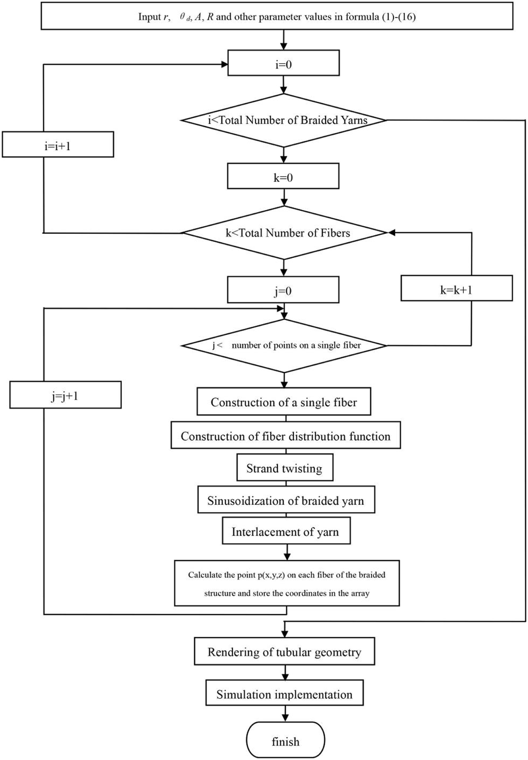
Flowchart of model construction.

Results of simulation

Two-dimensional circular fiber-level braided fabric

Figure 15 illustrates a 3D simulation of a 2D circular fiber-level braided fabric with 12 braided yarns (each braided yarn has six fibers). Figure 15(a) to (d) show braids made from strand units of braided yarns with different textures: (a) yarns with both Z-twist and S-twist, (b) all Z-twist yarns, (c) all S-twist yarns and (d) no twist. Figure 15(e) is braided from tape unit of braided yarns. Figure 15(f) is braided from polygonal cross-section of braided yarns. Figure 16 illustrates a 3D simulation of 2D circular fiber-level braided fabric with 12 braided yarns (each braided yarn has 16 fibers). The composition of braided yarns plays a crucial role in determining the various properties of fabrics. Different applications often lead to varying specific requirements for these fabrics. These factors need to be considered comprehensively in the design and production process. Figure 17 demonstrates the 3D simulation of a bent 2D circular fiber-level braided fabric, which is instructive for research related to braided ropes in pulley bending based on the finite element method.

Figure 15.

Two-dimensional circular braided fabrics (six fibers form with strand unit, tape unit). (a) S-twist + Z-twist. (b) Z-twist. (c) S-twist. (d) No twist. (e) Flat tape. (f) Polygonal cross-section.

Figure 16.

Two-dimensional circular braided fabrics (16 fibers form with strand unit, tape unit). (a) S-twist + Z-twist. (b) Z-twist. (c) S-twist. (d) No twist. (e) Flat tape. (f) Polygonal cross-section.

Figure 17.

Curved braid.

Variable cross-sectional fiber-level braided fabric

Matrix transformations are used to change the central coordinates around each monofilament in the cross-section of braided yarns. This allows for the creation of various multifilament yarn configurations, including flat, circular, and other cross-sectional shapes, resulting in the sinusoidal pathways of the braided yarns. Transformation matrices using different mathematical function expressions have been constructed to provide numerous movement trajectories for braided yarns. These diverse movement paths are essential in defining the outer contour shape of the braided fabric. Furthermore, the variable cross-sectional braided model may be expanded by changing the spatial trajectories of the points.

The variable cross-sectional braided fabric is obtained by using various mathematical function expressions to simulate the outer contour of the braided structure. Figure 18 illustrates a 3D simulation of variable cross-sectional braided yarns, specifically focusing on tape unit with multiple fibers.

Figure 18.

Variable cross-sectional braided fabric (tape unit). (a) Frustum of a cone. (b) Funnel. (c) Hyperbolic scanning body. (d) Drum. (e) Sphere.

Figure 18(a) to (e) show the variable cross-sectional braided fabrics in the shape of frustum of a cone, funnel, hyperbolic scanning body, drum and sphere, respectively. Figure 19 illustrates the 3D simulation of a variable cross-sectional braided fabric with 12 braided yarns of strand unit, consisting of 6 S-twisted yarns and 6 Z-twisted yarns.

Figure 19.

Variable cross-sectional braided fabric (strand unit). (a) Frustum of a cone. (b) Funnel. (c) Hyperbolic scanning body. (d) Drum. (e) Sphere.

Conclusion

This study offers a novel matrix transformation framework for fiber-level modeling of braided structures, enabling the transition from macroscopic to fiber scale. Unlike conventional point-by-point interpolation and the enhanced Frenet framework for modeling, the approach avoids computational redundancy, error accumulation and poor scalability. It features high computability with a clear and concise structure, uniform rules and excellent parameter scalability. A unified mathematical representation of fiber-level braided structures from single fibers to overall configuration has been achieved for the first time via analytical matrix transformations, significantly enhancing geometric adaptability and computational efficiency.

A scalable and systematic geometric model is developed for cross-scale modeling of single fibers, twisted yarns and intricate braided structures. The fiber distribution function is precisely solved using matrix operations and combined with important twisting parameters such as twisting degree, twist angle and twist direction to achieve accurate characterization of twisted yarn texture and improved 3D visualization. Construction of fiber-level braided structures is accomplished by precisely capturing the topological properties and spatial deformation during yarn interlacing through the variations in the outer contour and mandrel of braided structures. This multi-scale modeling enables flexible construction of braided structures, providing a reliable geometric basis for mechanical analysis and prediction of stiffness, strength, and deformation.

This model allows for flexible parameter settings by adjusting twisting parameters, fiber distribution function, floating length, total number of yarns in a group and outer contour shape function to simulate braided yarns with different fiber distributions and twists, fabrics with different braided structures, various outer contours and bending forms. The use of parameters embedded in the transformation matrix enables flexible adjustment of braided structures, further enhancing the applicability and flexibility of the model. The efficient mathematical modeling and parametric design method reduces the consumption of computational resources, shortens the development cycle of new products and facilitates the discovery of optimal design solutions.

Footnotes

Declaration of conflicting interests

The authors declared no potential conflicts of interest with respect to the research, authorship, and/or publication of this article.

Funding

The authors disclosed receipt of the following financial support for the research, authorship, and/or publication of this article: This work was supported by Postgraduate Research & Practice Innovation Program of Jiangsu Province (KYCX24_2573) and Natural Science Youth Fund project of Jiangsu Province (BK20221094).

ORCID iD

Ning Yang

References

Ding

Simulation of the hexagonal 3D braiding process for stent preforms. Text Res J 2024; 94(5–6): 691–703.

Xiao

Wang

Soulat

, et al Towards the deformability of triaxial braided composite reinforcement during manufacturing. Compos B Eng 2019; 169(7): 209–220.

Emonts

Grigat

Merkord

, et al Innovation in 3D braiding technology and its applications. Textile 2021; 1: 185–205.

Kyosev

Generalized geometric modeling of tubular and flat braided structures with arbitrary floating length and multiple filaments. Text Res J 2016; 86(12): 1270–1279.

Alpyildiz

3D geometrical modelling of tubular braids. Text Res J 2012; 82(5): 443–453.

Lomov

Ivanov

Verpoest

, et al Meso-FE modelling of textile composites: road map, data flow and algorithms. Compos Sci Technol 2007; 67(9): 1870–1891.

Huang

Causse

, et al Transverse compaction of 2D glass woven fabrics based on material twins – part I: geometric analysis. Compos Struct 2020; 237(4): 111929–111939.

Huang

Causse

, et al Transverse compaction of 2D glass woven fabrics based on material twins – part II: tow and fabric deformations. Compos Struct 2020; 237(4): 111963–111971.

Ghaedsharaf

Brunel

Lebel

LL.

Fiber-level numerical simulation of biaxial braids for mesoscopic morphology prediction validated by X-ray computed tomography scan. Composites, Part B 2021; 218(8): 1–11.

10.

Ghaedsharaf

Brunel

Laberge Lebel

Multiscale numerical simulation of the forming process of biaxial braids during thermoplastic braid-trusion: predicting 3D and internal geometry and fiber orientation distribution. Composites 2021; 150: 106637–106652.

11.

Kyosev

Braiding technology for textiles: principles, design and processes. Woodhead Publishing, 2014.

12.

Kyosev

Topology-based modeling of textile structures and their joint assemblies. Springer, 2019.

13.

Zheng

Huang

Modeling of 3D yarn in woven structure. J Textile Res (China) 2002; 23(2): 13–16.

14.

Qian

Analytical prediction of the elastic properties of 3D braided composites based on a new multiunit cell model with consideration of yarn distortion. Mech Mater 2016; 92: 139–154.

15.

Miao

Zhou

Wang

, et al Mechanics of textile composites: micro-geometry. Compos Sci Technol 2008; 68(7–8): 1671–1678.

16.

Leech

CM.

Theory and numerical methods for the modelling of synthetic ropes. Commun Appl Numer Methods 1987; 3(5): 407–413.

17.

Seo

Backer

, et al Structural modeling of double-braided synthetic fiber ropes. Text Res J 1995; 65(11): 619–631.

18.

Zhang

Beale

Adanur

, et al Structural analysis of a two-dimensional braided fabric. J Text Inst 1997; 88(1): 41–52.

19.

Ren

Gong

Liu

, et al Topology-based parametric modeling of three-dimensional hexagonal braids for advanced composite structures. Text Res J 2025; 95(1–2): 64–78.

20.

Stanova

Fedorko

Fabian

, et al Computer modelling of wire strands and ropes part II: finite element-based applications. Adv Eng Softw 2011; 42(6): 322–331.

21.

Ning

Potluri

, et al Geometrical modeling of tubular braided structures using generalized rose curve. Text Res J 2017; 87(4): 474–486.

22.

Ning

Computer-aided modeling of braided structures overbraiding non-cylindrical prisms based on surface transformation. Adv Eng Softw 2016; 98: 69–78.

23.

Rawal

Gupta

Saraswat

, et al Geometrical modeling of near-net shape braided preforms. Tex Res J 2015; 85(10): 1055–1064.

24.

Kamble

Behera

BK.

A novel geometric model of four-directional 3D braided preforms. J Ind Text 2022; 51(10): 1701–1715.

25.

Shao

Sun

Zhou

, et al Track design and realization of braiding for three-dimensional variably shaped cross-section preforms. J Eng Fibers 2021; 16: 1–11.

26.

Wang

Zhang

Shi

, et al Modeling method of irregular cross section annular axis braided preform based on finite element simulation. J Eng Fibers 2021; 16: 1–19.

27.

Guyader

Gabor

Hamelin

Analysis of 2D and 3D circular braiding processes: modeling the interaction between the process parameters and the pre-form architecture. Mech Mach Theory 2013; 69: 90–104.

28.

Rawal

Potluri

Steele

Geometrical modeling of the yarn paths in three-dimensional braided structures. J Ind Text 2005; 35: 115–135.

29.

Rawal

Potluri

Steele

Prediction of yarn paths in braided structures formed on a square pyramid. J Ind Text 2007; 36: 221–226.

Matrix transformation framework for modeling and analyzing braided structures

Abstract

Keywords

Introduction

Morphological characteristics and structure of 2D circular fiber-level braided fabrics

Morphological characteristics

Formation of braided structures

Geometrical modeling of 2D circular fiber-level braided structures

Assumptions

Generation of braided structures

Definition of geometric parameters

Construction of fiber distribution function

Mathematical modeling of strands

Parameter changes for mathematical modeling

Simulation platform construction

Model construction process

Results of simulation

Two-dimensional circular fiber-level braided fabric

Variable cross-sectional fiber-level braided fabric

Conclusion

Footnotes

Declaration of conflicting interests

Funding

ORCID iD

References