A heat-flow method for generating fiber placement trajectories over meshes

Abstract

Automatic Fiber Placement (AFP) is a principal processing method for carbon fiber reinforced composite materials and is widely applied in the contemporary manufacturing industry. An efficient and rational trajectory generation strategy is the crucial factor determining the quality and efficiency of fiber placement. This article investigates the effectiveness of employing numerical approximation in resolving the problem of determining fiber placement trajectories on triangular mesh molds. The proposed method, based on heat-flow (HF), can directly compute the distance map by solving a straightforward linear system and trace full coverage trajectories. It encompasses two pivotal processes, namely, enforcing initial boundary conditions and updating the vector field, and is capable of generating the expected full coverage equidistant trajectories without any gaps or overlaps. It can handle complex molds that are arduous to be expressed through parametric or implicit equations. The experimental simulation further substantiates the feasibility of the proposed method in generating full coverage trajectories and its potential application in AFP.

Introduction

At present, AFP has emerged as the primary processing approach for high-performance composites and is widely utilized in the domains of modern aircraft manufacturing. It possesses the capacity to operate each prepreg tow independently, and the width of the prepreg assembly can be adjusted in accordance with the surface characteristics and manufacturing requirements. Therefore, this technology is particularly suitable for the automatic molding of complex composite components, such as fuselage panels and S-shaped inlets, etc.^1,2 As an advanced and automatic manufacturing technology for fabricating fiber-reinforced composite components, an efficient and reasonable trajectory generation strategy, including the initial trajectory and offset trajectory, is the key factor determining the quality and efficiency of fiber placement and is directly related to the success or failure of fiber placement as well as the performance of the formed components.

Numerous efforts have been reported in the literatures addressing the generations of the initial trajectory and offset trajectory. For the generation of the initial trajectory, it can be generated with parametric functions, mapping the 2D curve onto the mold surface or projecting the reference path onto the mold surface. For the initial trajectory, a more classic one is the fixed direction (or fixed angle) method. The so-called fixed direction here implies that the trajectory has a fixed reference direction. Shirinzadeh et al^3–5 has provided detailed introductions to the working principle, trajectory planning, simulation, etc. of AFP. Taking the open surface as the object, a Surface Curve Algorithm that projects the reference line onto the mold surface is proposed to generate the initial trajectory. Wang et al^6,7 offered a similarly improved method called the APPSL algorithm with an arc-length parameter to construct the initial trajectory. In his method, the initial trajectory can be traced by solving first-order partial differential equations. Compared with the fixed angle paths, variable angles (or variable stiffness) trajectories are more customizable. Up to now, the main application objects of variable stiffness trajectories are some simple developable surfaces, such as plates, cylinders, cones, etc. Aimed at the composite laminated plate, Waldhart ⁸ proposed the variable stiffness trajectory design earlier and discussed in detail the curvature display, shear deformation response, etc. Based on the maximum principle stress vector field, Niu et al ⁹ adopted a sequence of uniform cubic B-spline segments passing through some given maxistress points as the initial trajectory. The other related studies can be found.^10–14 Aimed at the cone structure, Blom et al^15,16 provided the definitions of fiber trajectory and demonstrated the designed variable-stiffness trajectories based on the maximum fundamental eigenfrequency. Moreover, aimed at the cylinder structure, Jose ¹⁷ applied the variable stiffness trajectory of plates to design and optimize composite cylinders with a variable-axial layout under axial compression for the adopted design space, loads and boundary conditions. Similar works can also be referred to Blom et al.’s. ¹⁸

For the offset trajectory, the commonly employed methods are the translation method and the parallel method. The translation method can readily result in gaps and overlaps. Although Blom et al ¹⁸ proposed that the cutting and refeeding function of the filament winding machine could be utilized to avoid unnecessary fiber overlaps and gaps, it is undeniable that this will have an impact on the filament winding efficiency. Hence, researchers are mostly devoted to the study of the parallel method. Shirinzadeh et al ⁴ presented the SCO algorithm to offset the AFP trajectories along the surface a distance of one tow-width in a perpendicular direction. Similarly, Xiaoping et al ⁶ developed a technique named the APPSL algorithm with an arc-length parameter to offset trajectories. The offset trajectories are obtained by solving a first-order partial differential equation. Yan et al ¹⁹ presented a method to generate offset trajectories with a variable offsetting distance. Schueler et al ²⁰ calculated the points at an equal distance from the reference path by applying the method of replacing the arc length with the chord length, and then fitted these points to obtain the offset trajectory.

Although the abovementioned methods have achieved favorable results and have been applied to a certain extent in practice, the above trajectory generation strategies mainly focus on molds with explicit expressions (parametric surfaces and implicit surfaces). They typically have the following several shortcomings. (1) The obtained trajectories usually rely on precise mathematical expressions, which are often hard to obtain. (2) When dealing with situations where the trajectories exceed the mold boundary or are incomplete, complex intersection issues between the offset trajectories and the mold boundary must be addressed. (3) The applied methods cannot effectively handle molds with holes. (4) Some methods directly use chord lengths, etc. instead of the offset width, resulting in unnecessary gaps and overlaps (as shown in Figure 1). Consequently, to solve the above problems, this paper presents a new concept for generating AFP trajectories. That is, instead of the precise expression that traditional methods highly depend on, the mold is discretized into triangular meshes. A numerical method, namely the HF method, is adopted to calculate the initial trajectory and offset trajectory.

Figure 1.

Gaps and overlaps between two placement fibers. Left: equidistant; Middle: overlap; Right: gap. Here, the red curves are the placement trajectories.

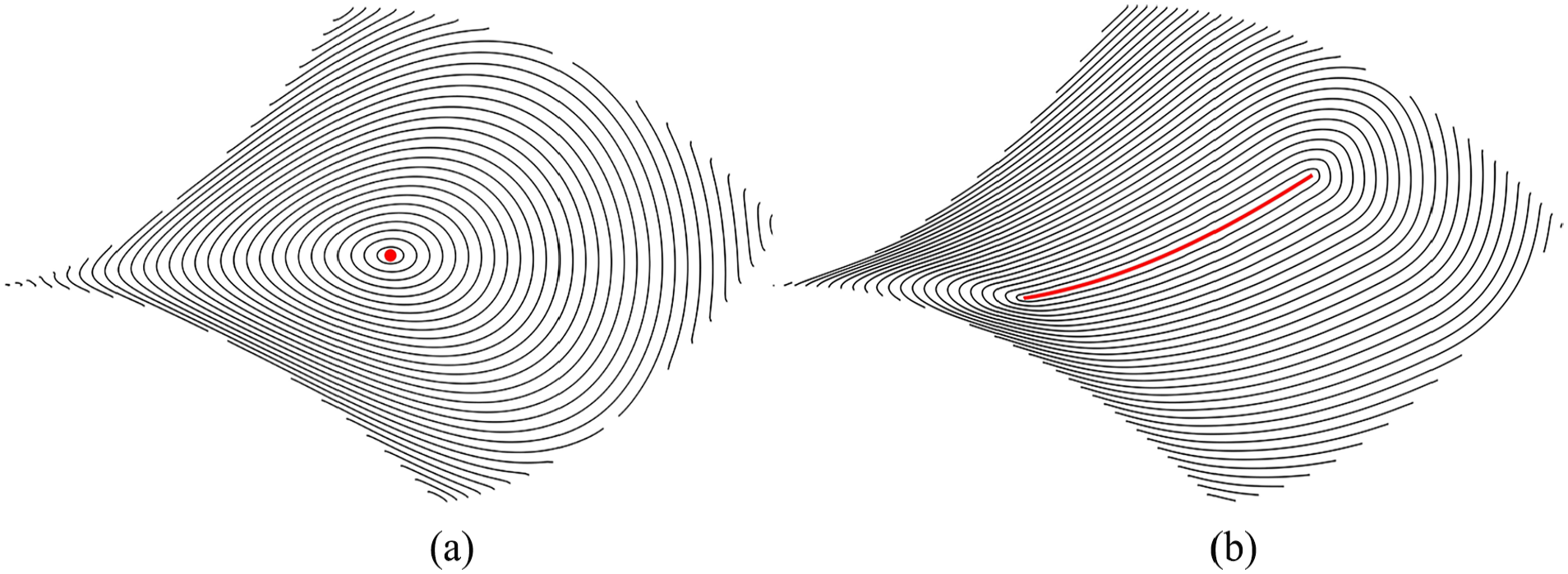
The proposed method relies on the initial boundary $\gamma$ , which can either be a single node on the boundary or a continuous point-set over the molds (as shown in Figure 2). Here, one can imagine a hot needle pointing to a node or countless needles pointing to a continuous curve on the molds simultaneously. Over time, the heat flow will spread across the molds and can be utilized to measure the shortest distance from any position to $\gamma$ . Therefore, the proposed method can be categorized as a geodesic method. For the case where the boundary $\gamma$ is multi-point (i.e. the form after the initial trajectory is discretized), it will automatically produce a series of equidistant full coverage trajectories that are applicable for AFP without gaps and overlaps. Moreover, since the propagation direction of the heat flow is often perpendicular to the fiber placement direction, which can serve as a natural input of the finite element method, one can directly carry out structural analysis targeting the final composite components. ²¹ Most importantly, our solvers only involve sparse linear systems that can be prefactored once and rapidly re-solved multiple times. All these advantages indicate that our method is particularly valuable for the trajectory generation of AFP.

Figure 2.

Computing distance isolines in relation to a specified boundary $\gamma$ (labeled in red). The black curves indicate the distance isolines: (a) $\gamma$ is a single node and (b) $\gamma$ is a node-set.

This article is organized as follows. Section 2 introduces the HF method. Section 3 elaborates on the generating steps of full coverage trajectories, including tracing the initial trajectory, enforcing the initial boundary conditions, modifying the vector field and tracing the equidistant trajectories. Some validation cases are illustrated in Section 4. The conclusions are drawn in Section 5.

The HF method

In this section, the HF method is introduced to provide a better comprehensive of the entire paper.^22,23 It can be employed to calculate the geodesic distance with respect to a specified boundary $\gamma$ (a node or node-set, as shown in Figure 2) on a mold surface described by triangular meshes. The overall steps are summarized as the Algorithm.1 related to a discrete gradient ∇, divergence ∇⋅ and Laplace operator $\mathrm{\Delta }$ .

Algorithm 1 The HF method
1: Integrate the heat flow $\stackrel{.}{u}=\mathrm{\Delta }u$ for fixed time $t$ . 2: Evaluate the vector field $X=-\nabla u/\left|\nabla u\right|$ . 3: Solve the Poisson equation $\mathrm{\Delta }\varphi =\nabla \cdot X$ .

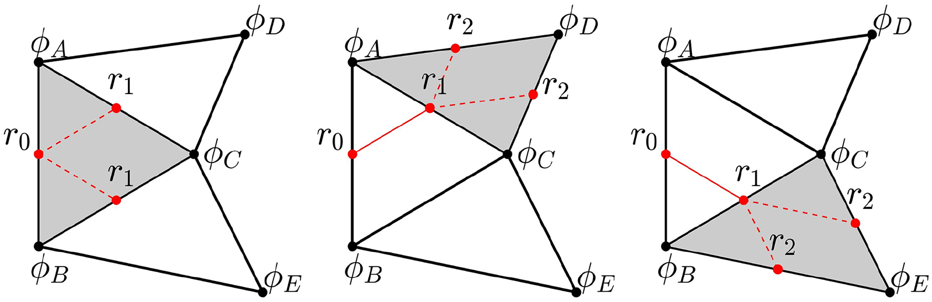
Let $\mathrm{\Omega }$ be a bounded computational domain related to the triangular mesh mold surfaces(mesh surfaces for short, same hereinafter) and $\mathrm{\Gamma }$ be the boundary of $\mathrm{\Omega }$ . The topology of a mesh surface $\mathrm{\Omega }$ is defined through a set of indexes $V=\{1,2,\cdots ,n\}$ that represent the $n$ nodes, a set of edges $E\subset V\times V$ and a set of elements $F\subset V\times V\times V$ . First, the Laplacian at a node $i\in V$ is discretized by

$${\left(L_u\right)}_i=\frac{1}{2A_i}\sum _j\left(\cot {\alpha }_{ij}+\cot {\beta }_{ij}\right)\left(u_j-u_i\right),$$

where $A_i$ is $1/3$ the area of all elements incident on node $i$ and the sum is taken over all neighboring nodes $j$ (see the left of Figure 3). Heat flow $u\in {\mathrm{ℝ}}^V$ can then be computed by solving the system

$$\left(A-t{L}_c\right)u={\delta }_{\gamma },$$

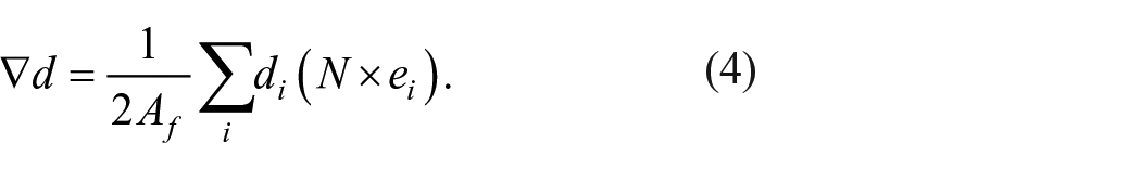
where ${\delta }_{\gamma }$ is a Kronecker delta over the boundary $\gamma$ , $A\in {\mathrm{ℝ}}^{V\times V}$ is a diagonal matrix for the area and $L_c\in {\mathrm{ℝ}}^{V\times V}$ is the cotan operator. The gradient (see the middle of Figure 3) for an elements is

$$\nabla u=\frac{1}{2A_f}\sum _i{u}_i\left(N\times e_i\right),$$

(1)

where $A_f$ is the element area and $N$ is its unit normal. The divergence (see the right of Figure 3) for node $i$ is

$$\nabla \cdot X=\frac{1}{2}\sum _j\cot {\theta }_1\left(e_1\cdot X_j\right)+\cot {\theta }_2\left(e_2\cdot X_j\right),$$

where the sum is taken over incident element $j$ each with a vector $X_j$ . Let $b\in {\mathrm{ℝ}}^V$ be the vector for the divergences of $X=-\nabla u/\left|\nabla u\right|$ , then the final distance function $\varphi \in {\mathrm{ℝ}}^V$ is computed by solving the symmetric Poisson problem

$$L_c\varphi =b.$$

Figure 3.

Calculation of geometry information.

In this article, we took the time step as $t=h_E^2$ , where $h_E$ represents the mean distance of all edges in $E$ .

Full coverage trajectories

The definition of equidistant trajectories is based on the solution of Eikonal equations

$$\nabla \varphi \left(\mathbf{x}\right)\approx -\frac{\nabla u}{\parallel \nabla u\parallel },\mathbf{x}\in \mathbf{\Omega }/\gamma ,$$

(2)

$$\varphi \left(\mathbf{x}\right)=0,\mathbf{x}\in \gamma \subset \mathbf{\Omega }.$$

(3)

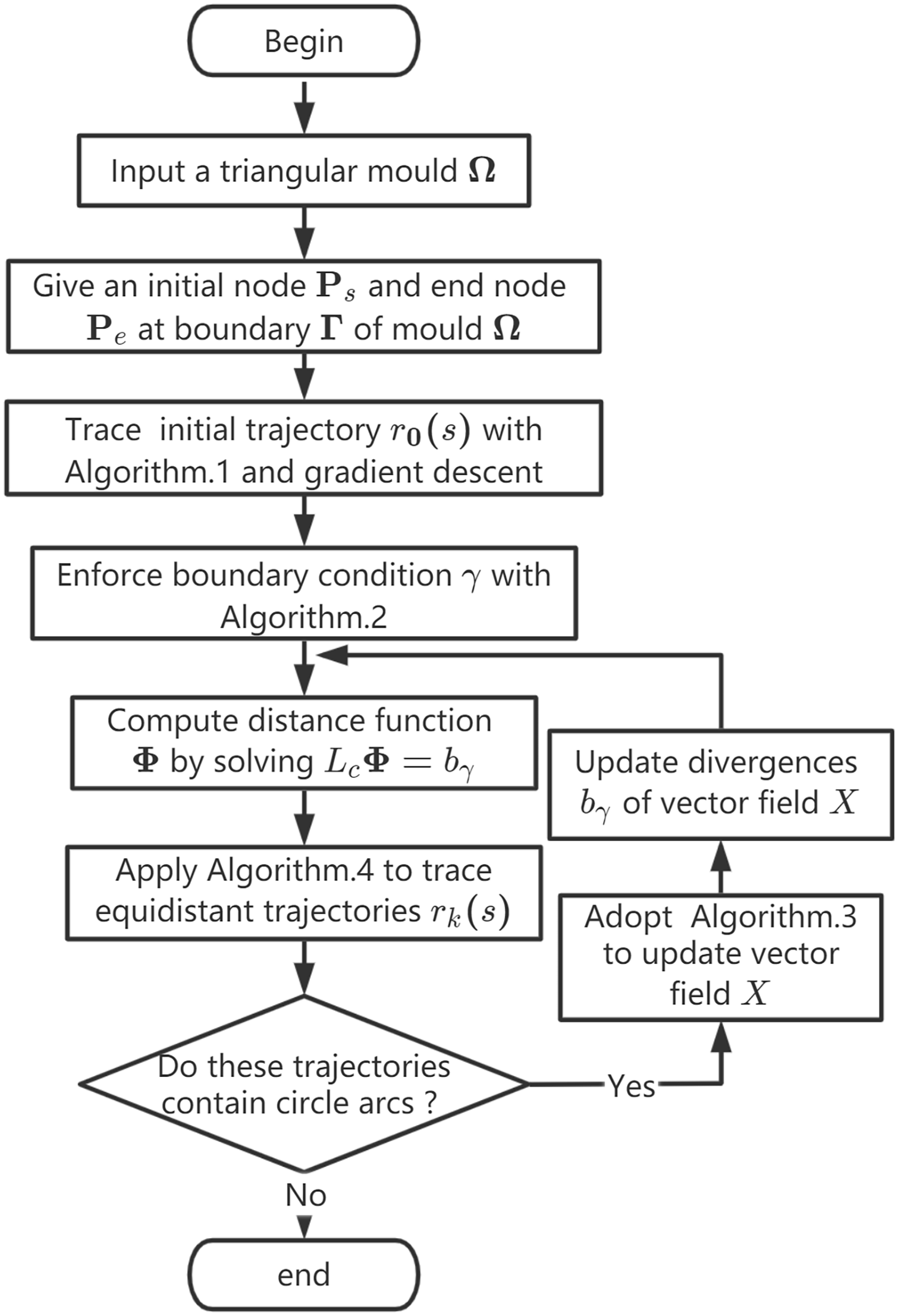
It can be solved using the Algorithm 1 and the overall steps are illustrated in Figure 4. Therefore, the generation of equidistant trajectories depends on the fact that the level set of the geodesic distance function $\varphi$ . ²³

Figure 4.

Outline of the heat method: (a) heat $u$ is allowed to diffuse for a brief period of time, (b) the temperature gradient $\nabla u$ is normalized and negated to obtain a unit vector field $X$ pointing along geodesics, and (c) a function $\varphi$ whose gradient follows $X$ recovers the final distance. (a) $u$ , (b) $\nabla u$ , (c) $X$ , and (d) $\varphi$ .

Tracing initial trajectory

There exist various candidates for generating an initial trajectory $r_0\left(s\right)$ : an isoparametric curve, a well-defined curve mapped onto mesh surfaces, a surface-plane intersecting curve and a curve that follows the line of principle stress. In this article, we employed the geodesic traced by the HM method as the initial trajectory $r_0\left(s\right)$ (see Figure 5). In this case, the boundary $\gamma$ is regarded as a singer node located at $\mathrm{\Gamma }$ , that is γ = P _s  ∈ R³ and the final solution $\varphi$ approximates the true geodesic distance over the mesh surface $\mathbf{\Omega }$ . Final values typically need to be shifted such that the smallest distance is zero(i.e. ${\varphi }_{\gamma }=0$ ). Because there are some negative values in distance function $\varphi$ and it generally meets ${\varphi }_{\gamma }=\min \left\{\varphi \right\}={\varphi }_{min}<0$ . One can trace the initial trajectory $r_0\left(t\right)$ with the updated distance function $\varphi -{\varphi }_{min}$ .

Figure 5.

Tracing the initial trajectory with gradient descent. The distance map $\varphi$ is computed by the HF method on the boundary $\gamma ={\mathbf{P}}_s$ . These black lines are geodesics between the start-point ${\mathbf{P}}_s$ and multiple end-points ${\mathbf{P}}_e$ .

Since the bounded computational domain $\mathrm{\Omega }$ is discretized by triangular meshes, the initial trajectory $r_0\left(s\right)$ having two end-points ${\mathbf{P}}_s,{\mathbf{P}}_e\in {\mathrm{ℝ}}^3$ located at $\mathrm{\Gamma }$ is composed of a series of discrete line segments embedding in elements $F$ . The arc parameter $s$ belongs to the interval $[0,s_{max}]$ , where $s_{max}$ is the length of the initial trajectory $r_0\left(s\right)$ . It is difficult to acquire the mathematical equations of such an initial trajectory $r_0\left(s\right)$ . But one can trace this trajectory from any node on $\mathrm{\Gamma }$ to the start point P _s using a gradient descent. ²⁴

Enforcing boundary conditions

For generating full coverage trajectories, it should be noted that the boundary $\gamma$ herein is not a single node in $\mathrm{\Omega }$ but a node-set (as shown on the right of Figures 2 and 6) discretized by the initial trajectory $r_0\left(s\right)$ . However, the gradient descent ²⁴ typically can provide two distinct forms of the initial trajectory, namely the discrete and continuous forms (see Figure 6). Generally, the initial trajectory in the continuous form cannot be directly regarded as the boundary $\gamma$ since the two end-points of all line segments are on the edge of elements. But for the discrete form, the generated trajectories are serrate (see Figure 6(a)). Even if the HF method provides a series of equidistant trajectories, the final network is not applicable for AFP. The solution to this problem is to enforce boundary conditions on the continuous initial trajectory (see Figure 6(b)). The specific measure is that we directly take the nodes of the elements crossed by the initial trajectory $r_0\left(s\right)$ as the boundary $\gamma$ . To distinguish the case where the boundary $\gamma$ is a single node, we referred the distance function as $\mathrm{\Phi }\in {\mathrm{ℝ}}^V$ when the boundary $\gamma$ is a node-set. Our measures for enforcing boundary conditions are concluded in Algorithm 2:

Figure 6.

Generating equidistant trajectories based on a discrete or continuous initial trajectory $r_0\left(s\right)$ . Blue points are the boundary $\gamma$ , thick red lines are initial trajectory $r_0\left(s\right)$ and blue surfaces are elements crossed by $r_0\left(s\right)$ : (a) discrete form and (b) continuous form.

Algorithm 2 Enforcing boundary condition
1: Compute distance function ${\mathrm{\Phi }}_{\gamma }$ at boundary $\gamma$ . 2: Update vector field $X$ for elements crossed by $r_0\left(s\right)$ .

We computed the distance function ${\mathrm{\Phi }}_{\gamma }$ from step 1 of Algorithm 2 with the true distance. The operational basis is that the distance function $\mathrm{\Phi }$ of the initial trajectory $r_0\left(s\right)$ is assumed to be the minimal value, that is, ${\mathrm{\Phi }}_{r_0\left(s\right)}={\mathrm{\Phi }}_{min}$ . Therefore, the distance function ${\mathrm{\Phi }}_{\gamma }$ on the boundary $\gamma$ is computed with the true distance $d_{\gamma }$ from x_γ to $r_0\left(t\right)$ , that is ${\mathrm{\Phi }}_{\gamma }={\mathrm{\Phi }}_{min}+d_{\gamma }$ (see Figure 7). Then, the vector field $X$ of the elements crossed by $r_0\left(s\right)$ can also be updated with equation (4). Here, the gradient in a triangular element crossed by the initial trajectory $r_0\left(s\right)$ is computed by the true distance $d$ rather than the heat flow $u$ shown in equation (2), that is

$$\nabla d=\frac{1}{2A_f}\sum _i{d}_i\left(N\times e_i\right).$$

(4)

Figure 7.

Update of vector field $X$ for an element ${\mathrm{\Delta }}_{ABC}$ . The red line is a segment $\{r_j,r_{j+1}\}$ of the initial trajectory $r_0\left(s\right)$ .

Finally, the vector field $X$ is updated with $X=-\nabla d/\left|\nabla d\right|$ . It should be noted that the distance function ${\mathrm{\Phi }}_{\gamma }$ that we expect over the boundary $\gamma$ is stable. Therefore, an accurate solver named “1” substitution method ²⁵ is adopted to solve the sparse systems $L_c\mathrm{\Phi }=b_{\gamma }$ to keep ${\mathrm{\Phi }}_{\gamma }$ fixed, where $b_{\gamma }\in {\mathrm{ℝ}}^V$ is an updated vector of divergences for the updated vector field $X$ .

Modifying equidistant trajectories

The HF Method can provide a set of equidistant trajectories over $\mathrm{\Omega }$ , but they cannot be employed as the final full coverage trajectories for AFP. From the situation presented in Figure 8(b), the initial trajectory $r_0\left(s\right)$ is a bounded curve. The other equidistant trajectories are propagated within the band defined by the two orthogonal lines at the two endpoints(P _s and P _e ) of the initial trajectory $r_0\left(s\right)$ . The domain outside this band is filled with circle arcs, as shown in Figure 8(b). The reason for this this is that the length of the initial trajectory is not infinite but bounded. Generally, one can choose the longest geodesic over mesh surface $\mathrm{\Omega }$ in the fiber placement direction as the initial trajectory $r_0\left(s\right)$ (such as the diagonal of a square, see Figure 6(b)). We are unable to accurately trace the longest geodesic for a complex or irregular mold in general, even if the curvature of these molds is small.

Figure 8.

Propagation of an initial trajectory $r_0\left(s\right)$ with the Algorithm 1 on a square plate. The red thick line is the initial trajectory and thin lines are the equidistant trajectories: (a) vector field $X$ and (b) equidistant trajectories with circle arcs.

We addressed this problem by locally modifying the vector field $X$ of the elements where the trajectories are circle arcs. For a mesh surface with a small curvature (such as a plane), one can directly take the vector field $X$ as a normalized vertical vector of the initial trajectory at P _s or P _e (see Figures 8(a), 9(a), and 11(a)). This procedure is simple and only suitable for flat surfaces. But for a complex surfaces, this procedure will lose its advantage. In this situation, an iteration method to update vector field $X$ is available and can be summarized as the Algorithm 3.

Figure 9.

Two different methods to update vector field $X$ . The red lines are initial trajectories $r_0\left(s\right)$ and the yellow surfaces are the cutting surfaces that split the domain with circle arcs: (a) direct method and (b) iterative method.

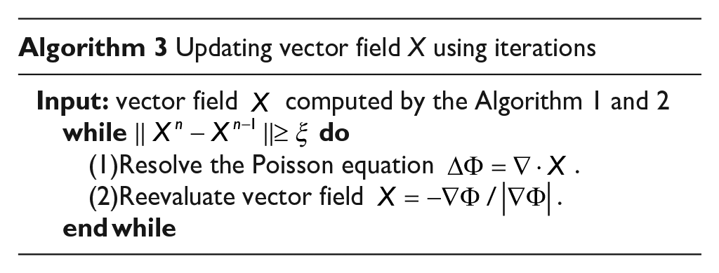
Algorithm 3 Updating vector field X using iterations
Input: vector field $X$ computed by the Algorithm 1 and 2  while  $\parallel X^n-X^{n-1}\parallel \ge \xi$  do   (1)Resolve the Poisson equation $\mathrm{\Delta }\mathrm{\Phi }=\nabla \cdot X$ .   (2)Reevaluate vector field $X=-\nabla \mathrm{\Phi }/\left|\nabla \mathrm{\Phi }\right|$ .  end while

The update of the vector field $X$ with iterations can be motivated as follows. It merely requires that the gradient $\nabla \mathrm{\Phi }$ points in the correct direction, that is, parallel to the propagation direction of the fibers. The magnitude can be safely disregarded since we knew (from the Eikonal equation in equations (2) and (3)) that the gradient of the true distance function $\mathrm{\Phi }$ has a unit length. This is similar to the gradient $\nabla u$ of heat flow propagation. We therefore updated the vector field with the normalized gradient field $X=-\nabla \mathrm{\Phi }/\left|\nabla \mathrm{\Phi }\right|$ and found the correct distance function $\mathrm{\Phi }$ based on the initial trajectory $r_0\left(s\right)$ by solving the corresponding systems $\mathrm{\Delta }\mathrm{\Phi }=\nabla \cdot X$ .

When performing the iteration of vector field $X$ in step (2) of Algorithm.3, we took the true distance between the boundary element (labeled in blue in Figure 9(b)) and the isosurface to update the gradient. Let ${\mathrm{\Delta }}_{ABC}$ be the updated element on the boundary $\mathrm{\Gamma }$ and ${\mathrm{\Phi }}_A$ be the distance function at node $A$ . One can construct an isosurface passing through three non-collinear nodes $Q_1\left(A\right),Q_2$ and $Q_3$ that meet ${\mathrm{\Phi }}_A={\mathrm{\Phi }}_{Q_2}={\mathrm{\Phi }}_{Q_3}$ (see Figure 10). If the three nodes are collinear, the isosurface is constructed by passing through nodes $Q_1,Q_2$ and the normal vector of element ${\mathrm{\Delta }}_{ABC}$ . Then, one can update the distance function at node $B$ with ${\mathrm{\Phi }}_B={\mathrm{\Phi }}_A+d_B$ , where $d_B$ is the true distance between node $B$ and the isosurface. The distance of node $C$ can be updated similarly. Finally, one can update the new gradient of element ${\mathrm{\Delta }}_{ABC}$ by

$$\nabla \mathrm{\Phi }=\frac{1}{2A_f}\sum _i{\mathrm{\Phi }}_i\left(N\times e_i\right).$$

(5)

Figure 10.

Generation of isosurface.

The gradient of all elements having one edge on $\mathrm{\Gamma }$ (labeled green in Figure 9(b)) can be updated in sequence by the above strategies. One can acquire an ultimately convergent vector field $X$ through the iteration in Algorithm 3 (see Figure 11(a)). The final expected full coverage trajectories for AFP can be acquired simultaneously (see Figure 11(b)). Here, the $\xi =e^{-10}$ is an error limitation (threshold) and the errors of two adjacent iterations are evaluated by $errors=\parallel X^n-X^{n-1}\parallel$ or $\parallel {\mathrm{\Phi }}^n-{\mathrm{\Phi }}^{n-1}\parallel$ .

Figure 11.

Correct propagation of an initial trajectory for AFP on a square plate: (a) modified vector field $X$ and (b) correct equidistant trajectories.

Tracing AFP trajectories

All trajectories are piecewise line segments with respect to parameter $s$ . Each pair of two trajectories has an equidistant and fixed distance equal to the fiber width. Let $h$ denote the fixed fiber width. Then the total quantity of trajectories, including the initial trajectory $r_0\left(s\right)$ , is $m=\left({\mathrm{\Phi }}_{\max }-{\mathrm{\Phi }}_{\min }\right)/h$ , which can fully cover the entire surface $\mathrm{\Omega }$ . Each of these trajectories has an isochromatic distance function in sequence, that is, ${\mathrm{\Phi }}_k={\mathrm{\Phi }}_{\min }+k\cdot h\left(k=1,2,\cdots ,m-1\right)$ . One should trace these trajectories in discrete form $\left\{r_k\left(s\right)\right|k=1,2,\cdots ,m-1\}$ by applying the distance function $\mathrm{\Phi }$ . Therefore, for any distance function ${\mathrm{\Phi }}_k$ , the related trajectory $r_k\left(s\right)$ can be traced by the Algorithm 4, and its simple processes are illustrated in Figure 12.

Algorithm 4 Tracing trajectory with distance function $\mathrm{\Phi }$

while the $r\left(s\right)$ reaches the boundary $\mathrm{\Gamma }$ of $\mathrm{\Omega }$  do   if ${\mathrm{\Phi }}_A\le {\mathrm{\Phi }}_{\mathrm{x}}\le {\mathrm{\Phi }}_C(\mathrm{or}{\mathrm{\Phi }}_C\le {\mathrm{\Phi }}_{\mathrm{x}}\le {\mathrm{\Phi }}_A)$ then { $r_i$ on edge $AC$ } $r_i=A+\frac{{\Phi }_{\mathbf{x}}-{\Phi }_A}{{\Phi }_C-{\Phi }_A}\cdot \overrightarrow{AC}$   else{ $r_i$ on edge $BC$ } $r_i=B+\frac{{\mathrm{\Phi }}_{\mathbf{x}}-{\mathrm{\Phi }}_B}{{\mathrm{\Phi }}_C-{\mathrm{\Phi }}_B}\cdot \overrightarrow{BC}$   end if   Find an adjacent element of ${\mathrm{\Delta }}_{ABC}$ with common edge $BC$ or $AC$ and update this edge as $AB$ ;  end while

Figure 12.

Tracing trajectory based on the distance function $\mathrm{\Phi }$ , where the element labeled in gray is the element to be updated. The red lines are the target trajectories and dotted lines are the potentially updated trajectories.

For the initial node $r_0$ of each trajectories, one locates an element ${\mathrm{\Delta }}_{ABC}$ with an edge (assumed to be $AB$ ) on the boundary $\mathrm{\Gamma }$ , and the distance function of nodes $A,B$ satisfies ${\mathrm{\Phi }}_A\le {\mathrm{\Phi }}_{\mathbf{x}}\le {\mathrm{\Phi }}_B$ or ${\mathrm{\Phi }}_B\le {\mathrm{\Phi }}_{\mathbf{x}}\le {\mathrm{\Phi }}_A$ . Then the initial node of each trajectory is determined by

$$r_0=A+\frac{{\mathrm{\Phi }}_{\mathbf{x}}-{\mathrm{\Phi }}_A}{{\mathrm{\Phi }}_B-{\mathrm{\Phi }}_A}\cdot \overrightarrow{AB}.$$

It should be noted that there might be two or multiple piecewise trajectories with the same distance ${\mathrm{\Phi }}_k$ on both sides of the initial trajectory. One should search for more initial node $r_0$ to trace these trajectories. Moreover, if a trajectory reaches a node in the computational domain $\mathrm{\Omega }$ , then the three constants $\frac{{\mathrm{\Phi }}_{\mathbf{x}}-{\mathrm{\Phi }}_A}{{\mathrm{\Phi }}_B-{\mathrm{\Phi }}_A}$ , $\frac{{\mathrm{\Phi }}_{\mathbf{x}}-{\mathrm{\Phi }}_A}{{\mathrm{\Phi }}_C-{\mathrm{\Phi }}_A}$ and $\frac{{\mathrm{\Phi }}_{\mathbf{x}}-{\mathrm{\Phi }}_B}{{\mathrm{\Phi }}_C-{\mathrm{\Phi }}_B}$ are equal to $0$ or $1$ . One should replace these constants with $\epsilon$ or $1-\epsilon$ , where $\epsilon$ is typically taken as $e^{-10}$ . This situation is also applicable for tracing the initial trajectory $r_0\left(s\right)$ .

Numerical experiments

The proposed methods can theoretically be applied to any molds represented by triangular mesh. Hence, some numerical cases are provided in this section to verify their effectiveness. Actually, one can directly trace full coverage trajectories via a computed distant function $\varphi$ or $\mathrm{\Phi }$ . It encompasses the generation of the initial trajectory $r_0\left(s\right)$ (red thick curves) and its propagation trajectories $\left\{r_k\left(s\right)\right|k=1,2,\cdots ,m\}$ (red thin curves). Generally, the proposed method can be applied to any triangular mesh surfaces $\mathrm{\Omega }$ discretized by parametric and implicit surfaces. For simplicity, the testing mesh surfaces $\mathrm{\Omega }$ are discretized by two implicit surfaces, namely, a paraboloid mold

$$f\left(x,y,0.1\left(x^2+y^2\right)\right)=0,\left(-4\le x,y\le 4\right)$$

(6)

and a saddle mold

$$f\left(x,y,0.25\left(x^2-y^2\right)\right)=0,\left(-4\le x,y\le 4\right).$$

(7)

Matlab, a software with powerful data analysis and visualization capabilities, can interact effortlessly with commonly applied industrial software such as Abaqus ²⁶ and Catia. ²⁷ It is employed to construct the above testing molds and generate the expected AFP trajectories. Furthermore, Figure 13 elaborates on the generating processes of full coverage AFP trajectories in detail.

Figure 13.

Flow of generating full coverage trajectories over a mesh surface.

For the first example, Figure 14 shows the full coverage trajectories propagated by the longest initial trajectory $r_0\left(s\right)$ over the moudles $\mathrm{\Omega }$ (i.e. $r_0\left(t\right)$ is the surface diagonal). The vector field $X$ in this case is as expected and there is no need to apply Algorithm 3 for update or modification, as shown in Figure 13. Then, a distance function $\mathrm{\Phi }$ based on the steps of enforcing the boundary condition can be computed by simply solving a linear system $L_c\mathrm{\Phi }=b_{\gamma }$ . Supposing the distance function $\mathrm{\Phi }$ has been accurately evaluated, another advantage of the proposed method is that one can trace the full coverage trajectories based on the fiber width $h$ , as shown in Figure 15. Then, the quantity of trajectories can be reasonably assigned according to the individual demand. This aspect cannot be achieved by the traditional trajectory generating methods over implicit and parametric surfaces. Moreover, Figure 16 shows the fiber placement direction in each triangular element, which provides an input for the finite element analysis of the composite structure.

Figure 14.

Full coverage trajectories over paraboloid molds (top row) and saddle molds (bottom row) at ${45}^{\circ }$ and $-{45}^{\circ }$ fiber placement directions: (a) ${45}^{\circ }$ , (b) $-{45}^{\circ }$ , (c) ${45}^{\circ }$ , and (d) $-{45}^{\circ }$ .

Figure 15.

Full coverage trajectories with different fiber width h over paraboloid molds at 45° fiber placement directions. Here, we have $\parallel {\mathrm{\Phi }}_{max}-{\mathrm{\Phi }}_{min}\parallel =6.6941$ : (a) $m=6$ , (b) $m=11$ , (c) $m=16$ , and (d) $m=21$

Figure 16.

Fiber placement directions on all triangular elements for finite element analysis. Here, the placement direction of the initial trajectory is along the $\mathrm{\Omega }$ : (a) paraboloid mold and (b) saddle mold.

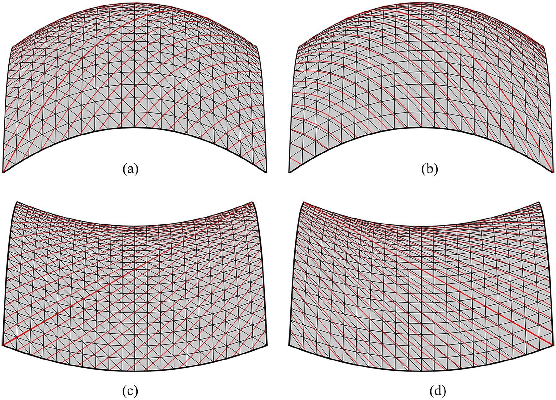
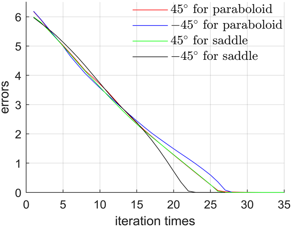
Figure 17 shows the case where the initial trajectory is no longer the longest curve for the mesh surfaces $\mathrm{\Omega }$ . Similar to Figure 7(b), the generated trajectories have some circle arcs. By applying the Algorithm 3, this problem can be readily addressed and an appropriate full coverage trajectories over ${45}^{\circ }$ can be obtained, as shown in Figure 17. Moreover, Figure 18 illustrates the decay of error with iteration in Algorithm 3. Here, the testing objects are the cases in Figure 17.

Figure 17.

Generating full coverage trajectories with Algorithm 3 over paraboloid and saddle mold when the initial trajectory is no longer the longest curve at fiber placement directions( ${45}^{\circ }$ and $-{45}^{\circ }$ ): (a) ${45}^{\circ }$ , (b) $-{45}^{\circ }$ , (c) ${45}^{\circ }$ , and (d) $-{45}^{\circ }$ .

Figure 18.

Iteration errors $\parallel {\mathrm{\Phi }}^n-{\mathrm{\Phi }}^{n-1}\parallel$ of Algorithm 3 for the four cases in Figure 17.

Figure 19 illustrates the full coverage trajectories over a complex mold with a hole. It further reveals the benefits of adopting a triangular mesh mold rather than a parametric or implicit mold. In this case, this mold is constructed by the paraboloid and saddle mold. The radius of its hole is taken as 1. However, it should be noted that this problem can actually be regarded as a multiple boundary problem. Different from the cases shown in Figure 17, we need to not only consider the boundary of the mold itself (labeled green on the left of Figure 19) but also the influence of the circular hole on generating the full coverage trajectories, because this circular hole will result in the trajectories with circle arcs. One has to consider the effect of all boundaries and need to update the vector field $X$ with Algorithm 3 along the circle hole (the blue curve on the right of Figure 19). The expected result can be seen in Figure 19. Furthermore, the proposed method is also applicable to industrial models. Figure 20 shows the full coverage trajectory on the aircraft tail wing.

Figure 19.

Full coverage trajectories over the molds with a hole at ${45}^{\circ }$ placement direction: (a) paraboloid mold, (b) expected results, (c) saddle mold, and (d) expected results.

Figure 20.

Full cover trajectories of the aircraft tail wing: (a) ${45}^{\circ }$ and (b) $-{45}^{\circ }$ .

So far, it is rare to apply triangular meshes instead of precisely expressed molds such as parametric surfaces or implicit surfaces for generating the initial trajectory and offset trajectory. It is undeniable that as a numerical method, the offset trajectories generated by the heat method will also have errors, thereby resulting in a certain proportion of gaps and overlaps. The error of the heat method is related to the parameter t. If $t=h_E^2$ , the error between the distance of the trajectory offset and the distance on the real surface is generally less than 1%. ²²

In order to verify the feasibility of implementation efficiency of the method in this paper, Table 1 presents the time for generating full coverage trajectories under different numbers n of mesh nodes. At the same time, it also provides a comparison of the efficiency with the classic literatures^4,6 on parametric surfaces. The generation of the initial trajectory relative to Shirinzadeh et al. ⁴ and Xiaoping et al. ⁶ can be acquired by projecting the straight line $P\left(t\right)=\left(0,0,6\right)+\left(0,1,0\right)t$ in the direction $\left(0,1,0\right)$ onto the mold of the paraboloid and saddle (as shown in equations (6) and (7)). After completing the aforementioned process with both methods, the results are gathered in a table form (as shown in Table 1).

Table 1.

Times(s) of generating full cover trajectories on the paraboloid and saddle molds.

Mold types	Methods	n	Paraboloid	Saddle
Parameter surface	4		1.6268	1.6456
	6		5.6970	5.6860
Triangular mesh	Ours	441	0.9721	0.9636
		1089	1.0171	1.0100
		6561	1.6597	1.5558

Conclusions

A numerical method based on the HF method is proposed for generating full coverage trajectories over mold surfaces described by triangular mesh. It not only focuses on the initial trajectory $r_0\left(s\right)$ , but also the subsequent propagating trajectories $r_k\left(s\right)$ . In this process, two crucial algorithms, namely, enforcing initial boundary conditions and updating the vector field $X$ , are developed. They can guarantee that the generated trajectories are equidistant without any gaps and overlaps, even when dealing with complex molds with multiple boundaries, such as holes that are difficult to express with parametric equations. Furthermore, all these traced trajectories are based on the distance map $\varphi$ or $\mathrm{\Phi }$ on mesh surfaces rather than parametric or implicit surfaces. Therefore, the fiber placement direction in each element can be directly calculated and utilized for finite element analysis. Most importantly, we can convert the complex problem of trajectory generation into solving a simple linear system related to the vector field $X$ . The numerical experiments in Section 4 have further demonstrated and verified the effectiveness of all the proposed strategies. Our investigation is mainly aimed at the geometric factor of mesh surfaces and combining the mechanical factor to generate full coverage trajectories that meet industrial requirements will be our future studies.