
Abstract
This article presents a layered decomposition method to decompose the machined surface into sub-surfaces with different components in dissimilar scale to identify machining errors. The high-definition metrology-measured data of the surface is first fitted by triangular mesh interpolation method to separate the surface into two sub-surface components, namely, system error caused and random error caused, respectively, whereas the stability of sub-surface entropy is used as the criteria to determine the refined mesh in case the decomposition exists throughout. Then, the sub-surface of system error is further decomposed by bi-dimensional empirical mode decomposition to get the error components varying in scales: surface roughness, waviness and profile, and as a result to identify the machining errors. Finally, self-correlation analysis is applied to each component to verify the decomposition. The result shows that each decomposed component has a distinctive wavelength, which proves that the method can successfully decompose the comprehensive surface topography into different scale components.
Keywords
Introduction
High-definition metrology (HDM) is one kind of non-contact measurement which enables inspecting a machined part surface at micron level with a high density of data up to million points. Figure 1 shows an engine head measured by HDM where the color indicates the height measurement (μm), and 2 million point data have been gathered. 1 High density of data information makes it possible to analyze the comprehensive topography of machined surface.
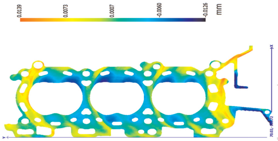
A V-6 engine head measured by HDM, Shapix Detective.
It is well known that the machined surface topography can influence many working characteristics of the part such as wear resistance, erosion resistance, anti-fatigue property, and optical property.2–5 So, it is a very important research to analyze the surface topography and unveil the formation of the surface.
Actually, the comprehensive topography of HDM surface formed under many factors’ synthetic action is generally composed by three distinct feature components, surface roughness, surface waviness, and surface profile, from small scale to large. The small-scale feature corresponds to the high frequency which reflects the surface residual irregularity, and it can be analyzed to judge the error from the process of removing the material. Large-scale feature is mainly caused by assignable reasons of machine tool so it can be used to identify those kinds of causes or system errors.6,7 Thus, it is necessary to divide the comprehensive surface topography into distinctive scales without distortion, which is the key to evaluate topography correctly. And statistically, the factors causing the errors of the machined surface during machining process can be sorted as random errors and system errors.
There are many studies in comprehensive surface topography separation from different perspectives. Least square method and B-spline surfaces express the surface topography as polynomial functions with the given polynomial coefficients, but these methods are only suitable for the continuous surface.8,9 Chen et al. 10 employed fast Fourier transform (FFT) analysis to deal with the measured data of spindle errors. Another kind of method treats surface topography as signal, and wavelet transform is used as an ideal method for multi-scale analysis. Liao 11 applied two-dimensional wavelet transform to three-dimensional (3D) cylinder head surface to get different scales of sub-surfaces which facilitates the revealing of process defects such as tool break, chatter, and potential leaking problem. Zeng et al. 12 proposed a double-tree complex wavelet to separate comprehensive surface and extract frequency component in different sub-surfaces. Wavelet decomposition was used by Zhao et al. 13 to divide turntable signals into low frequency and high frequency, and then, the low-frequency signal was used to trace the source of turntable mutation and saturation failure. Despite excellent performance of wavelet transform in multi-scale analysis of surface, there are some shortages in wavelet transform, which make it hard to use, such as how to choose the suitable wavelet basis and the number of scales.
Unlike wavelet transform affected by the choice of basis function and the determination of the decomposed levels, empirical mode decomposition (EMD) is another useful tool for surface decomposition which could realize signal adaptive decomposition according to its intrinsic characteristics without any consideration of basis function. Huang 14 used EMD to decompose signal into intrinsic mode functions (IMFs) varying in scales. Li et al. 15 applied EMD to decompose the error of ultra-precision grinding surface, getting distinct frequency range and Hilbert spectrum of each range was analyzed to find the errors and their causes. Bi et al. 16 obtained a set of intrinsic modes of optical surface by EMD and detected surface error and fluctuation frequency according to the characteristics of each mode.
Random error components can influence EMD decomposition result. It is essential to remove random error components from comprehensive surface topography to get assignable reasons causing system errors before using EMD. Least square method or B-spline is an ideal choice for removing random error of continuous surface topography, which is not suitable for non-continuous surface topography with some cavum on surface. This is because these methods just treat the spatial points as pure data, without considering the topological structure of spatial points.
In view of the above data, this article proposes a triangular mesh interpolation method to remove random errors of non-continuous surface and obtain the system error components. Then, EMD is applied to the system error causing surface to get different scales of sub-surfaces for the identification of the machining errors.
This article is structured in the following ways. Section “First-layer surface topography decomposition” discusses the first-layer surface decomposition to separate the system error and random error by triangular grid interpolation. The two-dimensional EMD method to fulfill the second-layer surface decomposition to get multiple intrinsic mode features is given in section “Second-layer surface decomposition—bi-dimensional empirical mode decomposition of system error.” Section “Result analysis” gives the actual machining process to analyze the intrinsic mode features and deduce the types of error sources for each modal. The summary of the article is given in section “Conclusion.”
First-layer surface topography decomposition
Modeling of the surface machining error
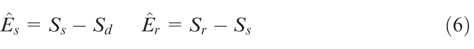
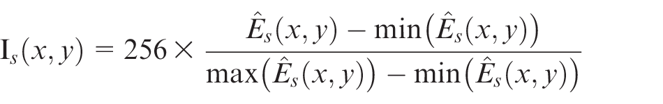
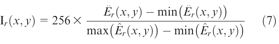
HDM such as Shapix1500 developed by Coherix, Inc. 17 can cover a section as large as 300 mm × 300 mm and generate a 3D height map point cloud within 40 s to describe a machined surface topography. The point cloud is shown in Figure 1. This gives us a possible way to model the surface machining error in detail. Surface topography error in general can be defined as the deviation between the designed surface and the actual machined surface
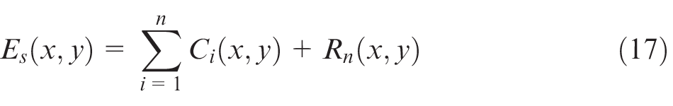
where
where
Triangular mesh fitting for random error decomposition
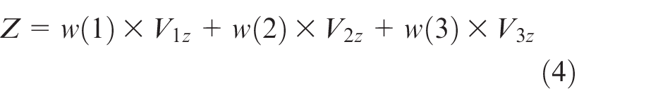
For continuous surface, least square fitting can be used to obtain the system error using polynomial to fit the surface points. But for non-continuous surface, if least square method or B-spline method is applied to get the system error, there must be some interpolation values in the discontinuous areas, while these areas have no corresponding values. Thus, the spatial information of surface points should be taken into account for non-continuous surface interpolation. The spatial information means that how the points are properly connected to a form triangular mesh. Figure 2(b) illustrates an incorrect points connection method for the formed mesh covering the hole shown in Figure 2(a); however, Figure 2(c) is a correct connection method avoiding mesh forming across the hole. The notion of forming triangular mesh from points is called point’s triangulation. There are many criteria to judge the characteristics of triangular mesh after triangulation to ensure the correctness of the point’s triangulation. Ensuring that circum circle associated with each triangle contains no other point in its interior is the basic requirement for the choice of the non-continuous surface triangular mesh. The mesh in Figure 2(b) and (c) is made by two algorithms, Lawson triangulation and Bowyer–Watson triangulation, to realize the triangulation, respectively. Here Bowyer–Watson triangulation is used for the HDM surface triangular mesh.
18
The result of triangulation is two data sets:
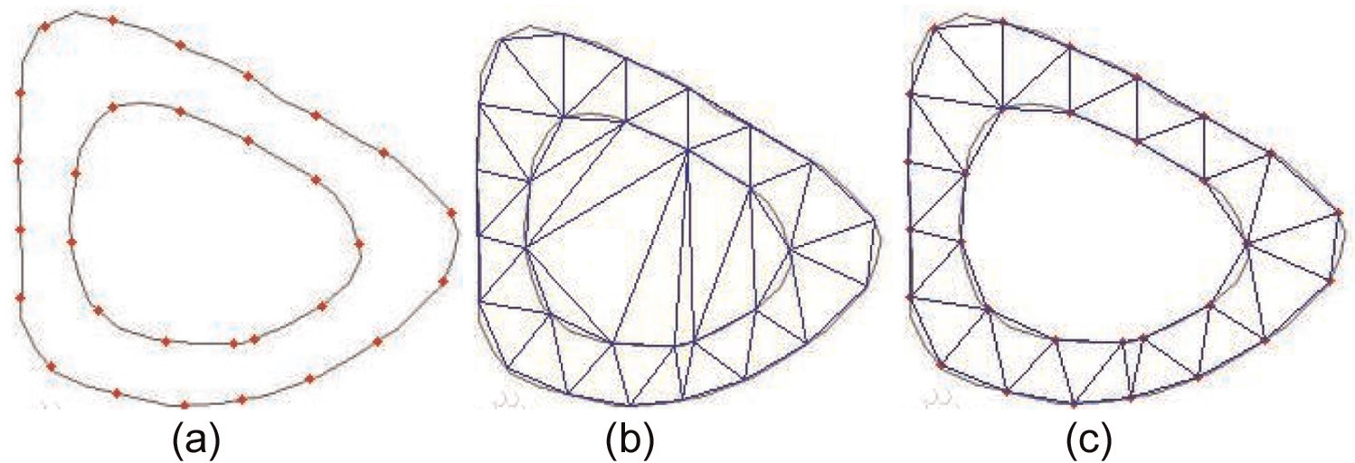
A demo of different triangular mesh algorithms: (a) surface points, (b) Lawson triangulation, and (c) Bowyer–Watson triangulation.
Triangular mesh interpolation algorithm
With the triangular mesh obtained in previous section, a triangular mesh interpolation algorithm is proposed to get the meshed surface for system error separation of non-continuous surface (Figure 3(a)–(c)). Every triangular net
Step 1. Number all the points of the triangular meshed surface, and all the
Step 2. Create a grid in XY plane for the meshed surface. In X-coordinate direction, the grid ranges from 0 to
Step 3. For each facet
Step 4. Calculate the weight
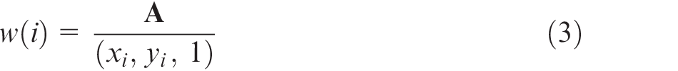
Step 5. Calculate the average height of the triangle as follows
Suppose every facet
where
A demo of triangular mesh interpolation: (a) number all the points, (b) create the grid, (c) find the smallest grid.
For any facet, the result of interpolation is to replace the original three vertices with one vertex value. As the point cloud usually has huge volume, interpolation can reduce this volume up to 2/3. For the noise points in the surface, once multiplied by the weight, make their impact small. It is the same effect as to smooth the surface by letting the surface topography pass through a low-pass filter. Thus by triangular mesh interpolation, the repetitive and redundant information was reduced, and random error was also eliminated. This provides a reliable assurance for EMD. So, the estimated value of the system error
Determining the number of triangular meshes
As mentioned in section “Triangular mesh fitting for random error decomposition” and equation (3), the estimated value of the system error is determined by the interval of grid. With changeable intervals of grid, a series of the estimated values of system error can be obtained ranging from rough to fine. Large intervals of grid can only get a rough approximation of the surface topography, which cannot completely describe the system error, whereas much small intervals of grid can give a very good approximation of the surface topography, which may effectively indicate good estimated system error as long as too much noise is not involved, but too much computing resources and time are needed. Therefore, it is necessary to find an ideal interval, namely, the suitable number of triangular meshes, which can correctly provide system error from surface while decreasing the random noise mixed in system error as small as possible. Here, entropy is used to determine the suitable number of triangular meshes.
Information entropy is first used to describe and measure the uncertainty of information source, and gradually, it is used to measure the uncertainty of random variables. The lower the probability of value, the lager its entropy. The largest entropy means largest uncertainty. The data with Gaussian distribution have the maximum entropy because there is almost no repeatable pattern and each value appears only once. Affected by system error and random error, surface topography follows Gaussian distribution. White House and Archand19,20 have proved that many engineering surface topographies have exponential self-correlation function relationship, which means surface topography has a repeatable and intrinsic pattern, and the entropy of system error should always be stable. So, set a larger grid interval for triangular mesh at first to get the estimated system error, random error, and their corresponding entropies, and then refine the interval every time to recalculate the entropy of new estimated system error until it becomes stable. This can be used as criteria to determine the suitable number of the triangular meshes. It is done as follows.
First, image entropy is introduced to calculate the entropy of system error and random error, as 3D surface topography can be treated as 2D image by the following method. And range of surface topography to 0–255 is mapped, as shown in Equation(7). The entropy of estimated system error and estimated random error can be calculated using the expressions as follows
and
where
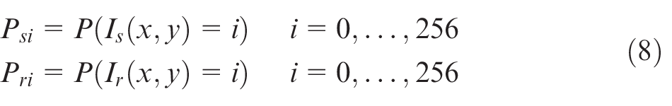
So, the entropies of the estimated system error and the estimated random error are
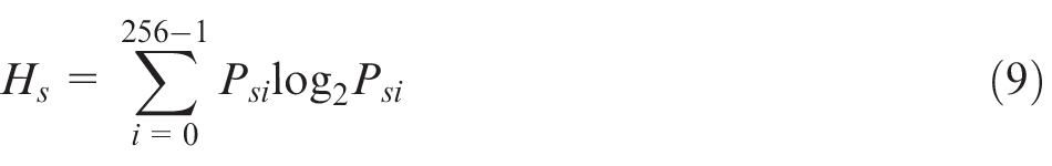
where
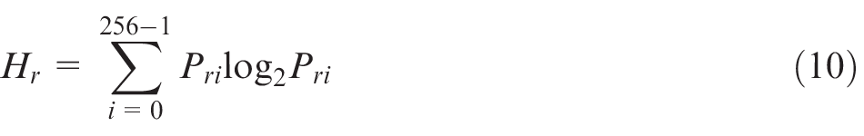
Relationship between entropy and grid quantity.
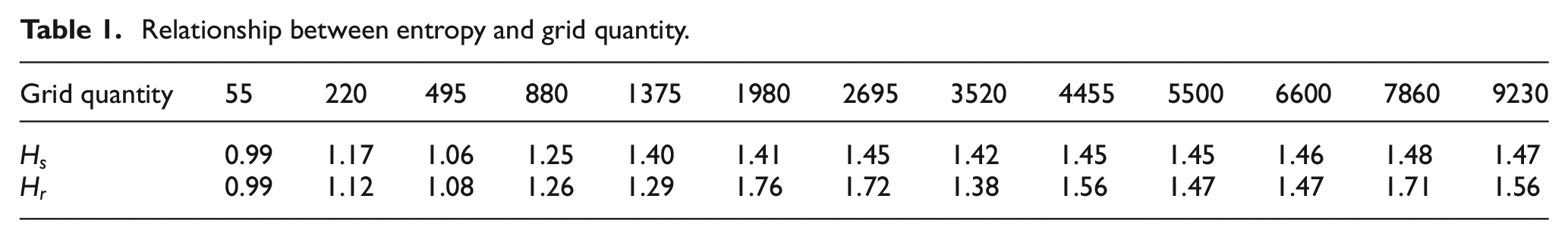
Entropy varies with the change in mesh quantity.
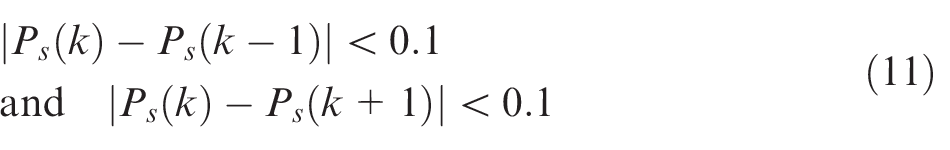
Figure 4 shows that entropy of the two kinds of errors is close to each other when the grid interval is large. As the interval decreases, the grid number increases, and the entropy of the estimated system error becomes stable, however that of random error presents fluctuation in certain region. The distinction between two entropies becomes obvious, which means system error can be extracted fully from surface topography. A criterion is given in equation (11) to quantify the “stable” condition of entropy of system error—for kth grid quantity corresponding entropy of system error
Then, the kth grid quantity can be used to get the system error completely without noise or redundancy. By this way, surface error E could be decomposed as random error and system error by the determined meshed surface
For the case shown in Figure 1, the grid quantity is 1980 and the stable entropy of the system error is 1.41; the system error and the random error are shown in Figure 5(a) and (b), respectively. To verify the thoroughness of the decomposition, an autocorrelation method is used. Figure 6 shows the exponential autocorrelation function of the obtained system error and random error. More than one peak point in Figure 6(a) shows the correlation among system error points which is the intrinsic feature of the system error, and only one peak point in Figure 6(b) shows the non-correlation of the random error point which also is the intrinsic feature of the random error. So, Figure 6 proves the correctness of the estimated value. And also, the mean values of
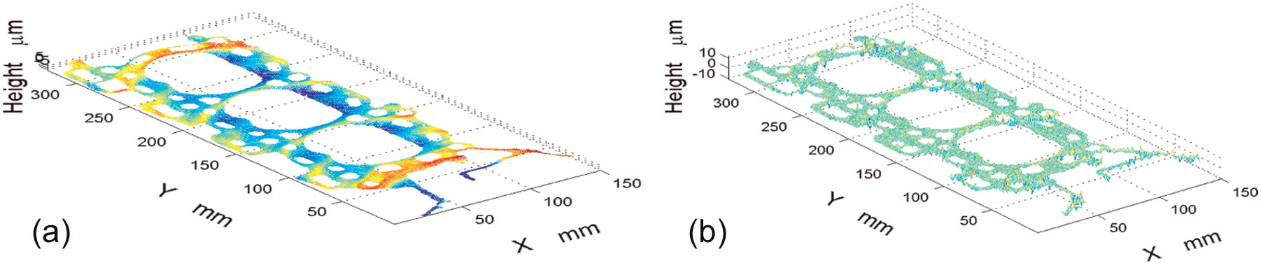
(a) System error and (b) random error from measured data.
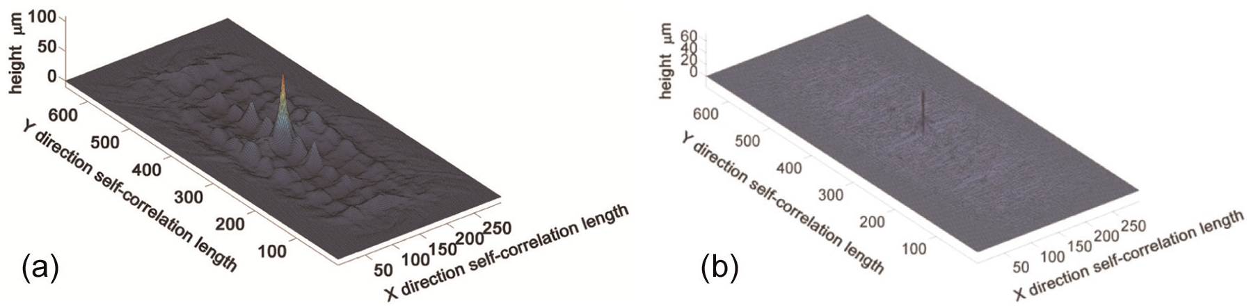
Self-correlation of (a) system error and (b) random error of surface.
Second layer surface decomposition—bi-dimensional empirical mode decomposition of system error
The system error may have many components varying in scale; it is necessary to separate them to single and intrinsic error type further according to their wavelength or frequency for machining error identification. Different scales’ error type is caused by different error sources varying in scale, thus there is definitely a mapping from error source to certain scale error type and the system is the linear superposition of different scale errors. Thus, system error separation is the foundation of evaluating surface topography and deducing error sources.
As the component of the entire surface topography, system error can also be treated as signal and the corresponding signal dealing method such as wavelet transform can be used here. As having a basic function to fulfill the filter function, wavelet transform may cause the separation results mixing with other frequency components or phase distortion when the improper basic function is used. 21 So, wavelet transform may be not the only one best choice to be used here. An ideal method for system error separation should have no predefined conditions such as basic functions and should make the system error to express all intrinsic error types “freely.”
EMD can well handle non-stationary, non-linear signal, by decomposing signal into multiple IMFs. Each intrinsic mode is an inherent component of a signal, and they are distinctive with each other in constitution. In the view of signal, surface can be seen as a non-stationary and non-linear signal because of the complexity of machining process. Thus, EMD is suitable for surface analysis. Here, two-dimensional EMD method is used which is similar to the one-dimensional EMD method. The hypotheses to use EMD are as follows: 22
The two-dimensional data plane contains at least one maximum and one minimum point or the whole plane does not have any extreme value point but after one or several derivative operations, there exists one maximum and one minimum point.
The characteristic scale is defined by the distance between those extreme values.
Similar to the one-dimensional EMD method, the decomposition screening process is as follows: Denote
The difference between the mean value and the primary is denoted as
where
By subtracting
Use
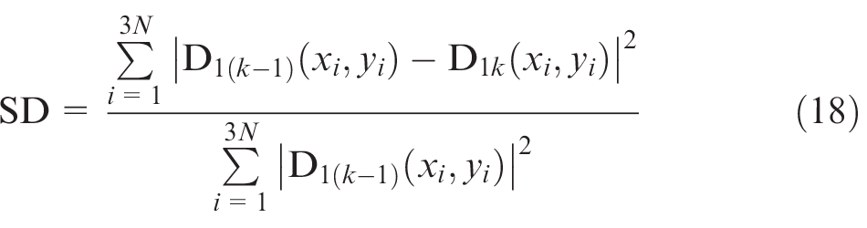
When the SD is smaller than the predefined value, the decomposition should be stopped. In general, SD takes the value between 0.2 and 0.3 and usually, the several former IMF components embody the significant information of the machining errors.
Result analysis
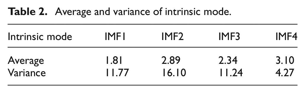
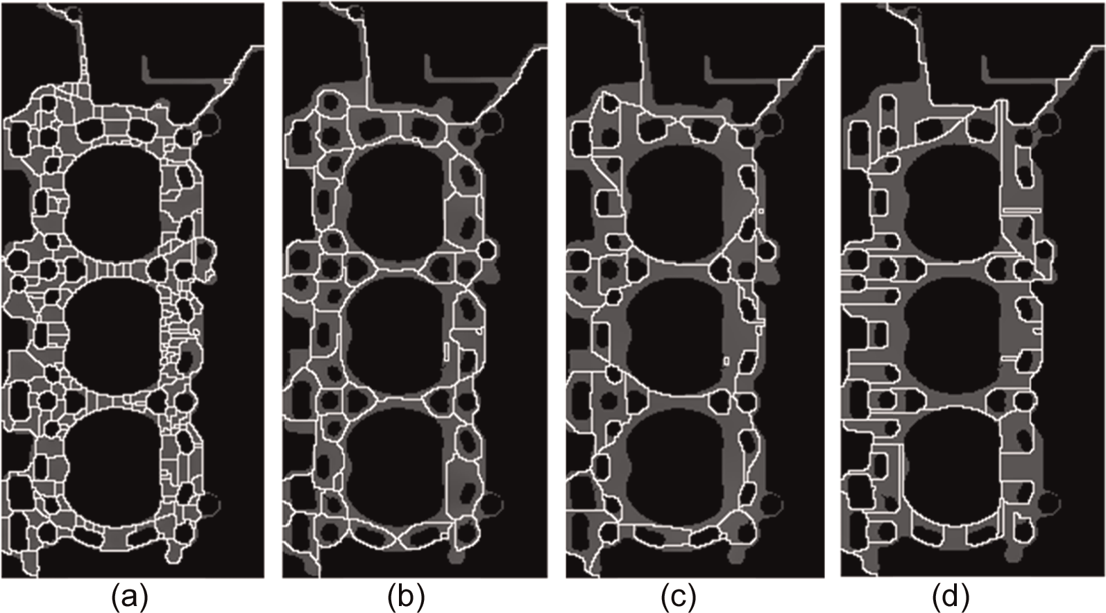
Taken the above engine head as an example, the system error was decomposed by bi-dimensional empirical mode decomposition (BEMD); one residual mode and three intrinsic modes were obtained as shown in Figure 7, and their mean value and variation are shown in Table 2. Each intrinsic mode represents one character of system error. Since these intrinsic modes are arranged from small scale to large scale, all of them represent roughness error, waviness error, and profile error. As the error sources are also with multi-scale character, every intrinsic mode corresponds to a certain error source. The analysis of intrinsic mode is helpful in deducing error sources during machining process.
Average and variance of intrinsic mode.
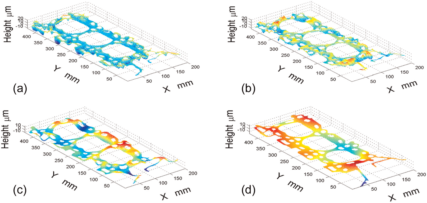
Intrinsic modes and residual of system error: (a) IMF1, (b) IMF2, (c) IMF3, and (d) IMF4.
Decomposition performance evaluation based on Moran’s I
Moran’s I statistical method performs effectively in spatial correlation analysis which is employed to verify the effectiveness and accuracy of the proposed method. Moran’s I ranges between -1.0 and 1.0 as a rational number after variance normalized. Moran’s
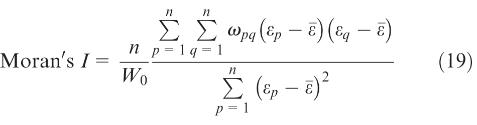
where
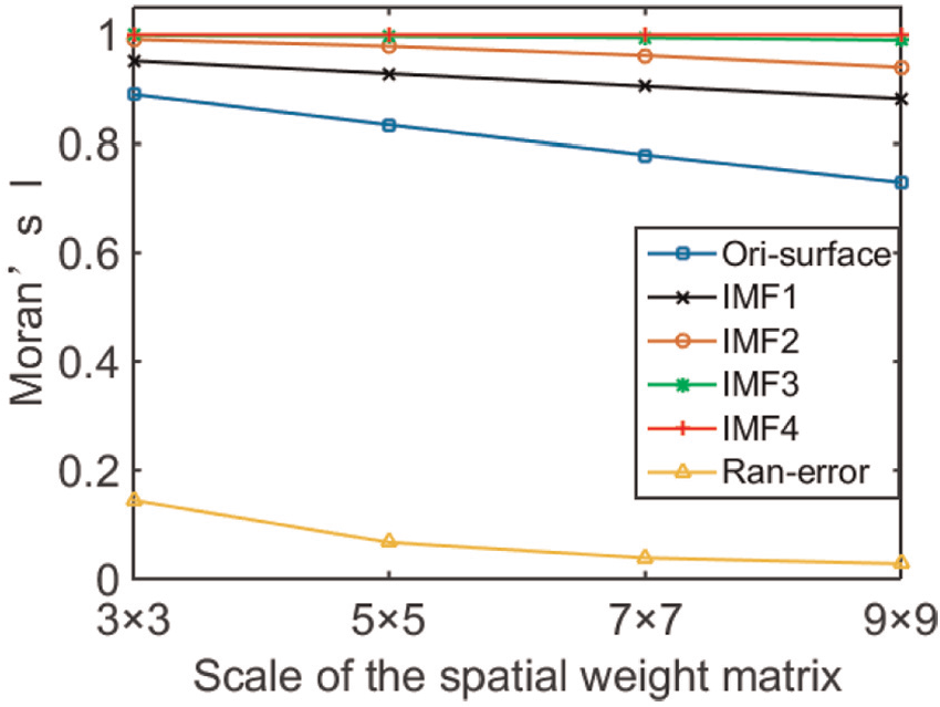
The original surface topography is decomposed into a random error and a system error which includes four sub-components: IMF1– IMF4. Moran’s I values of the original surface and the several components are calculated, and the results are shown in Figure 8. The horizontal axis denotes the scale of an inverse Euclidean distance spatial weight matrix and
Moran’s I index values of the different components.
From Figure 8, it can be seen that Moran’s I index value of original surface topography is around 0.8 and it declares that there is a kind of strong positive spatial correlation. The original surface topography data are still affected by some random errors which are caused by noises from machining and measurement process. And the Moran’s I of the random sub-components is below 0.2, which shows they are very low spatial correlation and this phenomenon means the sub-component is right in the random error. While for four IMFs sub-surfaces, their Moran’s I index values are near to 1, which indicate that they are strong positive spatial correlation. And this is the system error–related pattern. Those conclusions can also be drawn by wave components of the four IMFs shown in Figure 9. It can be deduced from Figure 9 that decomposed random error shows weak spatial correlation and decomposed system error sub-components show very strong positive spatial correlation. These results are in accordance with the expected ones. It verifies that the method effectively decomposes the original data into several systematic components and a random component.
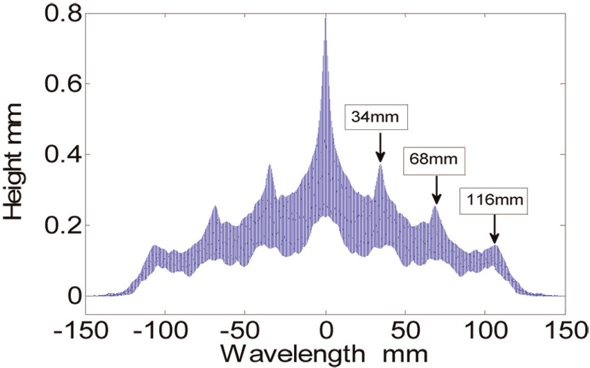
Wave components of system error for the machined surface.
Machining error identification based on self-correlation analysis and error texture analysis
As has been noted, machined surface has three different components in scale: roughness, waviness, and profile and they can be distinguished by their wavelength. 23 Some useful information can be obtained from the components are their wavelengths. The self-correlation of composite system error is first obtained, as shown in Figure 9. In the self-correlation diagram, the peaks corresponding to the horizontal axis value are the main wave’s wavelength, and the vertical axis denotes the amplitude of the wave. Self-correlation diagram is symmetric to origin 0. Figure 9 shows that the system error is mainly constituted by three kinds of waves, with a wavelength of 34, 68, and 116 mm, respectively. Besides, there is an obvious down trend in the right side of the figure. According to the character of self-correlation, it can be deduced that a large and slow-varying wave exists in the system error, which is one kind of system error: profile.
In this research, the self-correlation of each IMF in height direction and in width direction is calculated to get the main wavelength, as shown in Figure 10. At the same time, error texture analysis is employed besides self-correlation analysis which also contributes to identifying machining error. Error texture analysis originates from MOTIF method 24 and it can describe texture characteristics of the surface through linking local high points. Error texture results of four IMFs are shown in Figure 11.
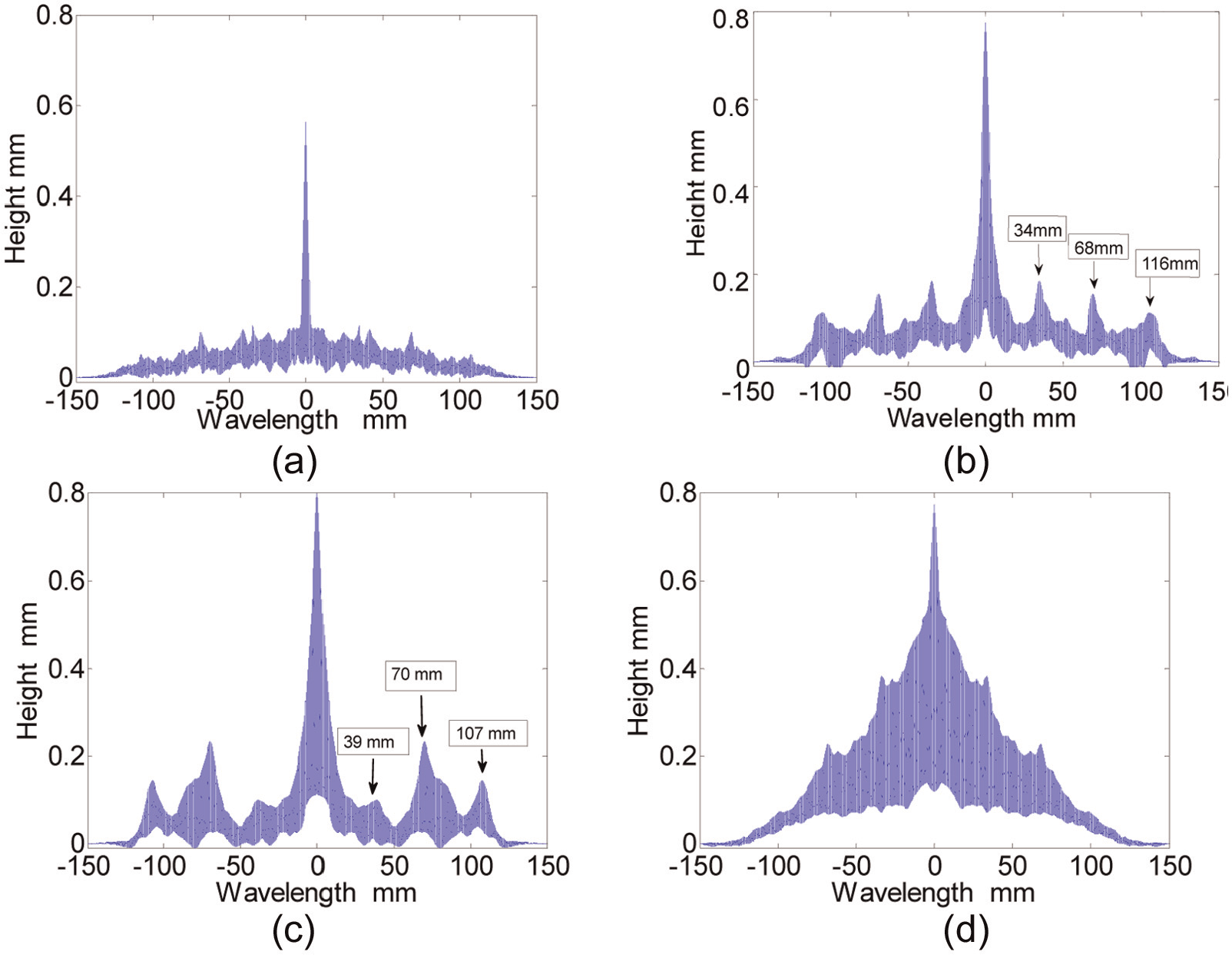
Self-correlation of IMFs: (a) self-correlation of IMF1, (b) self-correlation of IMF2, (c) self-correlation of IMF3, and (d) self-correlation of IMF4.
Error texture of IMFs by MOTIF method: (a) IMF1, (b) IMF2, (c) IMF3, and (d) IMF4.
As shown in Figures 10 and 11, IMF1 is the roughness components, with very small magnitude of waves. However, it has no obvious periodic wave and its error texture is cluttered, which is exactly the character of roughness.
IMF2 and IMF3, with obvious waves, are waviness components of system error. IMF2 has the same wavelengths with system error (Figure 9), which proved that the proposed method is valid. However, IMF3 has almost the same but slight distorted wavelength with respect to system error. This is caused by end effects of EMD method: 25 when cubic spline interpolation is applied to a limited signal, envelope curve distorts at two terminals, and the distortion will extend inside in the next iterations. But it did not have much effect for analysis in this article. The most interesting thing is the difference in IMF2 and IMF3. In IMF2, the 34-mm wave has a larger magnitude than that of 68- and 116-mm waves. According to its error texture shown in Figure 11(b), the phenomenon that texture evenly rounds all the holes in the surface is easily observed. The texture rounds can be classified as two main types by their sizes. One type rounds small holes and their sizes are close to 34 mm. Another type rounds the bigger cylinder holes and their sizes are close to 116 mm. A reasonable guess is that IMF2 is exactly produced by the effect from multi-holes structure to the machining process. While in IMF3, 39-mm (close to 34 mm) has a much small magnitude, and 70- and 116-mm waves are the dominating components. IMF3’s error texture tends to appear on the edges of the holes. Although both IMF2 and IMF3 have waviness components, they both show a different aspect of waviness.
IMF4 has no sign of wave but it has an obvious down trend on the right side of Figure 10(d), which indicates IMF4 with a large- and slow-varying shape: the profile of system error. In Figure 11(d), the texture shows the directionality along horizontal and vertical directions. The directionality indicates that IMF4 is mainly produced by location deviation. There is existing datum error or fixture error in machining process.
Conclusion
This article has three main contributions. First, it provides a new and feasible method to handle the discontinuous surface topography fitting problem. Many other arithmetic are currently used to fit continuous surface topography, which are not suitable to discontinuous surface. Second, from the information theory perspective, entropy has been used as criteria to determine the number of the triangular meshes in decomposition system error from random error. Third and the most important is that all the methods proposed in this research are optimized to get the best and stable performance, which means it can be directly applied to industrial parts’ surface inspection. Meanwhile, our future work will consider building relationship between decomposed machining error components and processing parameters. It will offer a methodology for improving machining precision and the error compensations.
Footnotes
Acknowledgements
The authors gratefully acknowledge the facilities provided by the Industrial Engineering Laboratory (IEL) at the Beijing Institute of Technology.
Declaration of conflicting interests
The author(s) declared no potential conflicts of interest with respect to the research, authorship, and/or publication of this article.
Funding
The author(s) disclosed receipt of the following financial support for the research, authorship, and/or publication of this article: This research was supported by the National Natural Science Foundation of China (NSFC grant no. 51275049) and the National Department Project (no. 613243).