Geometric modeling and simulation for leno fabrics

Abstract

The leno fabric is widely used in production and life for its distinctive style. However, its production and design are hindered by the unique weaving process. In this paper, a three-dimensional simulation algorithm is proposed to enhance the efficiency of leno fabric production. Three geometric models are constructed that systematically address different aspects of fabric simulation. The Yarn Spatial Trajectory Model, in which the centerline trajectory of the yarn is controlled by the weave matrix, allowing for the realistic simulation of intertwined yarns characteristic of leno structures. The Variable Coefficient Elliptic Cross-Section Model, by which yarn collisions are prevented and computational demands are reduced. The Multifilament Model, critical to rendering quality, accurately captures the textural characteristics of yarns and fabrics. Leno fabrics are simulated based on the above models. The simulation results show that: different yarn counts and twists, fabric counts, hexagonal hole sizes, and other simulation effects can be achieved by entering different parameters. By the 3D simulation algorithm developed in this study, simulation fabrics have clear textures, precise structures, and realistic visual effects, thereby advancing the technology of leno fabric production.

Introduction

Leno fabrics, unlike typical woven materials, utilize a dual system of warp yarns – straight and leno yarns. ¹ These are continuously rearranged by a specialized leno heddle device to create distinct, smooth holes on the fabric surface. ² This unique construction makes leno fabrics ideal for applications like summer clothing, high-end decorations, automotive interiors, mosquito nets, and medical supplies, where they are highly appreciated by consumers. Prior to mass production, rigorous proofing is necessary to confirm design precision.^3–5 However, the specialized weaving techniques and heddle devices used limit the efficiency of sample production, leading to higher costs in materials, labor, and time.^6–10 Consequently, there is a crucial need to enhance economic efficiency through advanced fabric simulation technologies.

Research in fabric simulation is broadly divided into three main categories. The first focuses on fabric structure. Lin et al. ¹¹ developed geometric algorithms for three-dimensional modeling of woven fabrics in TexGen software. They analyzed issues such as structure, yarn path, and cross-sectional shape in woven fabrics, ultimately establishing a more universal mathematical model. Zheng et al. ¹² investigated the geometric structure of plain woven fabrics based on mechanical principles, proposing a spring-slider model, and ultimately obtained the geometric structure of plain woven fabrics in a stable state. Turan and Başer ¹³ and Patumchat et al. ¹⁴ both considered the yarn deviation caused by the fabric structure and established geometric models for twill fabrics. These studies have contributed to the simulation of fabric appearance, but existing models often overlook non-orthogonal yarn intersections, failing to accurately represent leno fabrics.

The second category addresses the collision issues between yarns to improve fabric rendering. Barauskas and Kuprys ¹⁵ modeled the yarn as a spring chain and used the Oriented Bounding Box (OBB) algorithm to eliminate the permeation between yarns. Sherburn et al. ¹⁶ adjusted the spatial trajectory and cross-sectional shape of yarns using the finite element method and energy minimization method to avoid yarn permeation during the simulation process. Cirio et al. ¹⁷ discretized the interlacing points between yarns when simulating woven fabrics, addressing yarn collision issues by employing distance field implicit methods. The collision detection accuracy in the aforementioned studies is high. However, the algorithms are complex, with the majority of program runtime dedicated to resolving yarn collision issues.

The third category enhances the realism of fabric simulations by focusing on yarn and fabric texture characteristics. After establishing three-dimensional geometric models, applying texture mapping techniques^18,19 to map yarn characteristics onto cylinders can to some extent reflect fiber-level simulation effects. However, from a geometric perspective, yarns are still smooth cylinders. Wu et al. ²⁰ initially partitioned the microscopic images of fabrics into different rectangular units. Subsequently, they restored the geometric shapes of yarns through image shading and, finally, generated the yarns using algorithms. Zhao et al. ²¹ utilized physical CT measurements to obtain the centerline trajectories of yarns, employing geometric and statistical methods to generate hairness. These methods, collectively referred to as reverse modeling of fabrics, extract information from real images, resulting in highly realistic simulation outcomes. However, their drawback lies in their dependence on existing fabrics.

Given the complex structure of leno fabrics, there has been no previous study that simulates these fabrics in three dimensions. This paper systematically models leno fabrics by considering the above three perspectives. It aims to enhance the realism of virtual fabrics through three novel geometric models: the Yarn Spatial Trajectory Model, the Variable Coefficient Elliptic Cross-Section Model, and the Multifilament Model. These models leverage geometric methods known for their intuitiveness and computational efficiency. By adjusting the weaving matrix, we control yarn trajectories to accurately mimic the intricate leno structure. Additionally, we introduce a collision detection mechanism that prevents yarns from penetrating each other, based on the spatial geometric model of the fabric. We also develop a mathematical model at the fiber scale to capture the texture features of yarns, such as twist and direction. The leno fabric simulation algorithm introduced in this paper can be directly integrated into computer-aided design systems to reduce the fabric proofing cycle. Additionally, it offers valuable insights for both the education and production of leno fabrics.

Geometric model

Yarn spatial trajectory model

In this paper, the coordinate system used is the right-handed coordinate system, with the origin located at the center of the screen. The X-axis points to the right, the Y-axis points upwards, and the Z-axis points outward from the screen.

Fabric digitization

During the weaving process, the specialized leno device, as illustrated in Figure 1, continuously exchanges the positions of the straight yarn and leno yarn. To the left of the figure, the shed and reed directions are indicated. In the initial state shown in Figure 1(a), the leno yarn is positioned to the right of the straight yarn. Figure 1(b) shows the rear heald frame lifted, with the leno yarn still to the right of the straight yarn. Figure 1(c) illustrates the movement of the leno yarn around the straight yarn to the left side when the front heald frame is lifted. This alternating up-and-down cyclic motion of the front and rear heald frames, as depicted in Figure 1(b) and (c), creates the appearance of leno fabric.

Figure 1.

Schematic diagram of warps entwined under the leno device: (a) initial state, (b) rear heald frame lifted, and (c) front heald frame lifted.

Figure 1 depicts the formation of the leno structure, highlighting how the leno yarn wraps around the straight yarn. However, the straight yarn may shift from its original position due to the tension exerted by the weft yarns. It is assumed that during weaving, the positions of the straight and leno yarns continually interchange under the influence of the weft yarns. Essentially, the weaving process involves two warp yarns twisting around each other, resulting in a symmetrical relationship between the straight and leno warps upon completion of weaving. Figure 2 demonstrates this yarn deviation using two representative leno structures as examples.

Figure 2.

Schematic of straight warp deviation: (a)Type 1 and (b)Type 2.

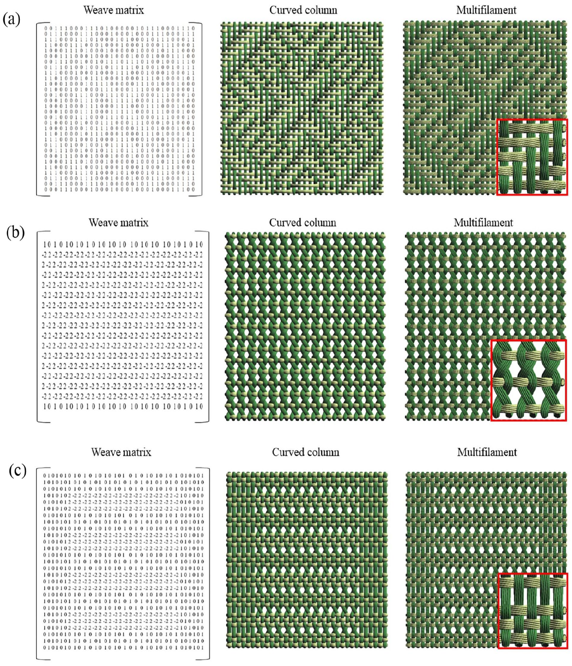
For standard single-ply woven fabrics, the weaving matrix typically uses “1” to denote warp interlacing points and “0” for weft interlacing points. ²² However, due to the complex structure of leno fabric, the traditional elements “0” and “1” are inadequate. To accommodate this, the elements “−2” and “2” are introduced, expanding the Boolean weaving matrix into a four-element matrix: “0,” “1,” “−2,” and “2.” In this system, “1” continues to represent a warp interlacing point in non-leno structures, and “0” signifies a weft interlacing point. For leno structures, where adjacent warp yarns twine around each other, “2” or “−2” are used to denote their interlacing points. Corresponding straight warp interlacing points are marked with the opposite element. Despite the warp yarns swapping positions from left to right during weaving, they revert to their original positions after the weave is completed. Therefore, in the weaving matrix, the elements “2” and “−2” are excluded from the first and last rows. Figure 3 illustrates how the leno structure is digitized into a weaving matrix.

Figure 3.

Digitization of the weaving chart.

Data points

In this study, we utilize the interweaving points of yarns and the midpoints between neighboring interweaving points as data points to generate the spatial trajectories of yarns in fabrics using spline curves. Figure 4 illustrates the distribution of these data points: • indicates the interweaving points of warp and weft yarns, while ○ represents the midpoints between two adjacent interweaving points, or the start or end points of the yarn. The notation Δd_warp denotes the center distance between two adjacent warp yarns. Δd_weft refers to the center distance between two adjacent weft yarns in conventional structures, and Δd_lenoweft specifies the center distance between two adjacent weft yarns in leno structures.

Figure 4.

Distribution of yarn data points.

If the fabric structure consists of m weft yarns and n warp yarns, the weave matrix is denoted as Matrix, which should comprise m rows and n columns of elements. To facilitate the calculation of yarn data point coordinates, start by creating a one-dimensional array weftDistArray to store the center distances between adjacent two weft yarns. The number of elements in the weftDistArray should be m−1. The storage rule is as follows: the distance between the (i−1)th and i-th weft yarns is stored in weftDistArray (where 0 < i < m). Owing to the distinctive attributes of the woven fabric structure, only two elements, Δd_weft and Δd_lenoweft, are stored within this array.

Due to the variation in fabric structure, different floats of yarn are formed, leading to changes in the yarn waviness. ²³ It is hypothesized that the z-value of the interlacing point (the coordinate value along the Z-axis) satisfies the relationship described by the following equation ²⁴ :

$$h_z=\sqrt{\left|f/2\right|+\frac{1}{2}}\times h_p$$

(1)

In equation (1), h_z represents the z-value height of the interlacing point, f denotes the length of the floating length line, and h_p indicates the yarn waviness when the interlacing point is located in the plain structure. When the warp yarn is entwined, its floating length line length remains 1, implying that the height of the interlacing point remains h_p.

Coordinates of weft data points

Noting the weft data points matrix as WeftMatrix, the matrix (containing 3D coordinates of interweaving points, intermediate points, start and end points) should have m rows and 2n + 1 columns. Each element in the matrix WeftMatrix represents a 3D coordinate point (x, y, z). WeftMatrix[i,j].x, WeftMatrix[i,j].y, and WeftMatrix[i,j].z represent the 3D coordinates (x, y, z) of the jth data point of the ith weft yarn in the weft data point matrix WeftMatrix, respectively. Let WeftMatrix[i,0].x be a constant t1; the calculation method of the x-value for this matrix element should be:

$$\begin{array}{l}WeftMatrix[i,j].x=t1+\frac{j}{2}\cdot \Delta d_{warp}\\ 0\le i<m,0<j\le 2n\end{array}$$

(2)

In the aforementioned equation, i and j represent the subscripts of the matrix. Let WeftMatrix[0, j].y be denoted as the constant t2, and the calculation of the y-value should be performed as follows:

$$\begin{array}{c}WeftMatrix[i,j].y=WeftMatrix[i-1,j].y\\ -weftDistArray[i-1]\\ 0<i<m,0\le j\le 2n\end{array}$$

(3)

The calculation for the z-value is as follows:

$$WeftMatrix[i,j].z=\{\begin{array}{ll}sign\cdot h_z& j\%2=1and\left|Matrix[i,j/2]\right|\ne 2\\ -WeftMatrix[i-1,j].z& j\%2=1and\left|Matrix[i,j/2]\right|=2\\ \frac{WeftMatrix[i,j-1].z+WeftMatrix[i,j+1].z}{2}& j\%2=0\end{array}$$

(4)

In equation (4), where i ranges from 0 to m−1 and j ranges from 1 to 2n−1; the sign function, denoted as sign, takes on a value of 1 when Matrix[i, j/2] equals 0, and a value of −1 when Matrix[i, j/2] equals 1. When both WeftMatrix[i,0]. z and WeftMatrix[i,2n].z (weft start and end points) are set to 0, the z-values for all weft data points can be determined.

Coordinates of warp data points

Noting that the warp data points matrix is WarpMatrix, the matrix (comprising three-dimensional coordinates of interweaving points, intermediate points, start and end points) should have 2m+1 rows and n columns. Similar to the data matrix of weft yarns, each element in the WarpMatrix represents a 3D coordinate point (x, y, z). WarpMatrix[i,j].x, WarpMatrix[i,j].y, and WarpMatrix[i,j].z correspond to the 3D coordinates (x, y, z) of the ith data point of the jth warp yarn in the warp data point matrix WarpMatrix, respectively. The y-value calculation for the warp matrix element is as follows (j = 0. . .n−1):

$$WarpMatrix[i,j].y=\{\begin{array}{ll}t2+\frac{1}{2}\Delta d_{weft}& i=0\\ t2& i=1\\ WarpMatrix[i-1,j].y-\frac{1}{2}weftDistArray[i/2-1]& 1<i<2m\\ WarpMatrix[i-1,j].y-\frac{1}{2}\Delta d_{weft}& i=2m\end{array}$$

(5)

When calculating the z-value of the warp yarn interweaving points(i%2 = 1), consider “2” as “1” and “−2” as “0,” the z-value is calculated as (i = 1. . .2m−1, j = 0. . .n−1):

$$WarpMatrix[i,j].z=\{\begin{array}{ll}-sign\cdot h_z& i\%2=1\\ \frac{WarpMatrix[i-1,j].z+WarpMatrix[i+1,j].z}{flag\cdot 2}& i\%2=0\end{array}$$

(6)

In equation (6), flag serve as a marker. When either element of Matrix[i/2−1,j] or Matrix[i/2,j] has an absolute value of 2, the value of flag is −1. For all other cases, the value of flag is 1. Let WarpMatrix[0,j].z and WarpMatrix[2m,j].z (the starting and ending points of the warp) both be 0. This allows us to determine the z-values for all data points of the warp.

The calculation of the warp x-value is essential for simulating the apparent of fabric. Initially, warp yarn entwined is not taken into account, and all warp yarns are treated as parallel aligned threads. The x-value of the interweaving point and the starting and ending points of the warp yarns can be expressed as (j = 0. . .n−1):

$$WarpMatrix[i,j].x=t1+\frac{1}{2}\Delta d_{warp}+j\cdot \Delta d_{warp}i\%2=1ori=0ori=2m$$

(7)

In this paper, it is assumed that the straight warp and leno warp are in a symmetric relationship after weaving is completed (refer to Figure 2). Therefore, after calculating the x-values of the parallel warp yarns, it is still necessary to adjust the x-values of the two adjacent entwined warp yarns by incorporating the weaving matrix. The pseudo code diagram of the warp winding algorithm is shown in Figure 5, flag1 is a boolean variable with an initial value of false.

Figure 5.

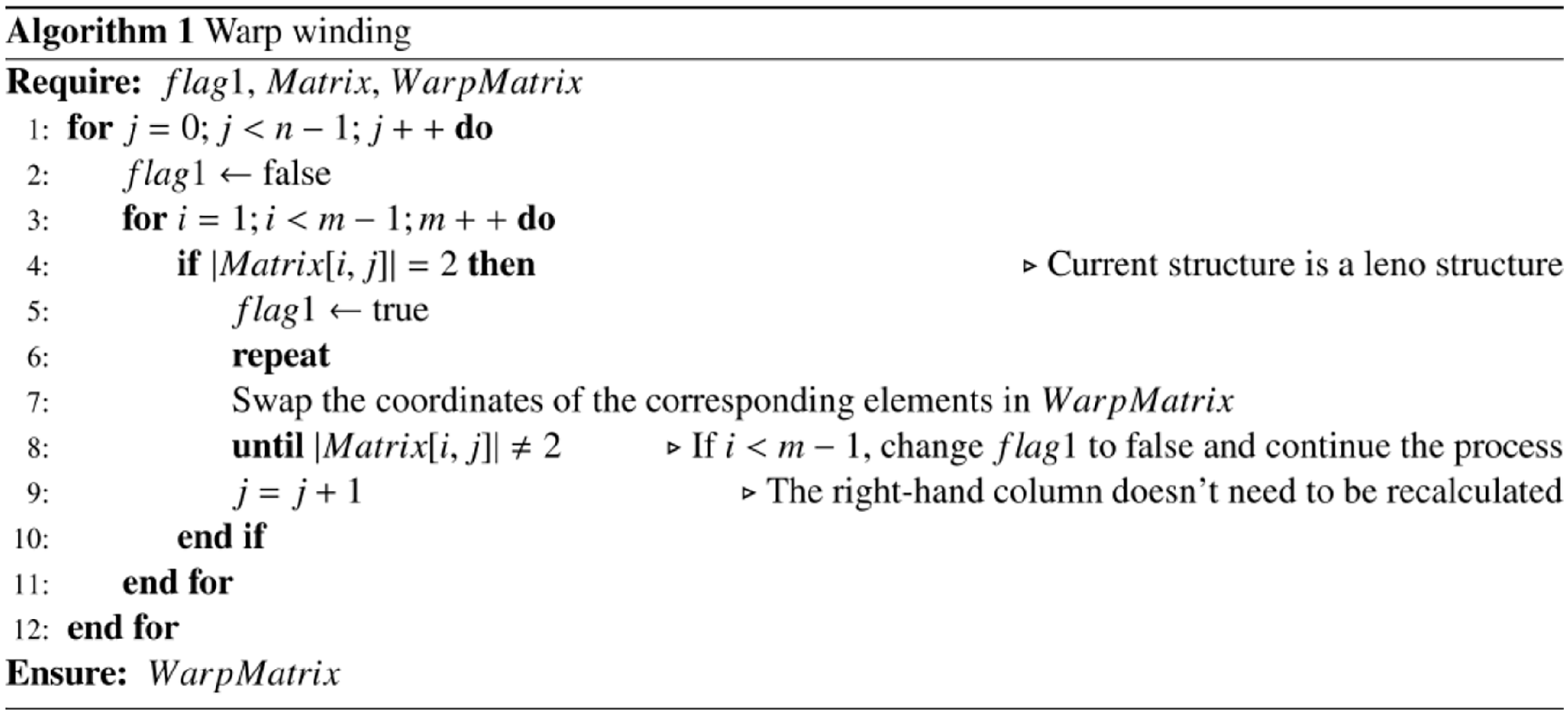
Pseudo code diagram of the warp winding algorithm.

After determining the x-values of the interlacing point coordinates, the x-coordinates of the interlacing points can be obtained by averaging the x-values of two adjacent interlacing points along a yarn. Figure 6 illustrates the simulation process of the leno structure curved cylinder based on the algorithm described above. This trajectory is obtained after the data points, generated under the influence of the weave matrix, are fitted using the spline curve.

Figure 6.

Fitting of yarn trajectories and leno structure simulation.

Variable coefficient elliptic cross-section model

The yarn spatial trajectory model previously established effectively simulates leno structures. However, in scenarios with high fabric density, collisions between yarns can degrade the simulation quality. Typically, yarns have a circular cross-section in their free state, but they deform during weaving due to extrusion and collision with other yarns. It is hypothesized that this deformation transforms the yarn’s cross-section into a continuously changing ellipse. To address this, we have developed parametric equations for a spatial ellipse, inspired by plane rotation and translation. Consequently, a variable coefficient elliptic cross-section model has been formulated, taking into account the forces at the yarn’s interweaving point and the spatial geometry of the yarn.

Parametric equation of spatial ellipse

Figure 7 illustrates the rotation of the Oxy plane within the Oxyz coordinate system to the plane defined by the equation cosα x+cosβ y +cosγ z = 0 (α, β, and γ are the angles between the normal vector of the plane and the positive directions of the X, Y, and Z axes, cos²α+cos²β+cos²γ = 1, and cosγ ≠ 1). In this configuration, ON represents the normal vector of the rotated plane, expressed as (cosα, cosβ, cosγ).

Figure 7.

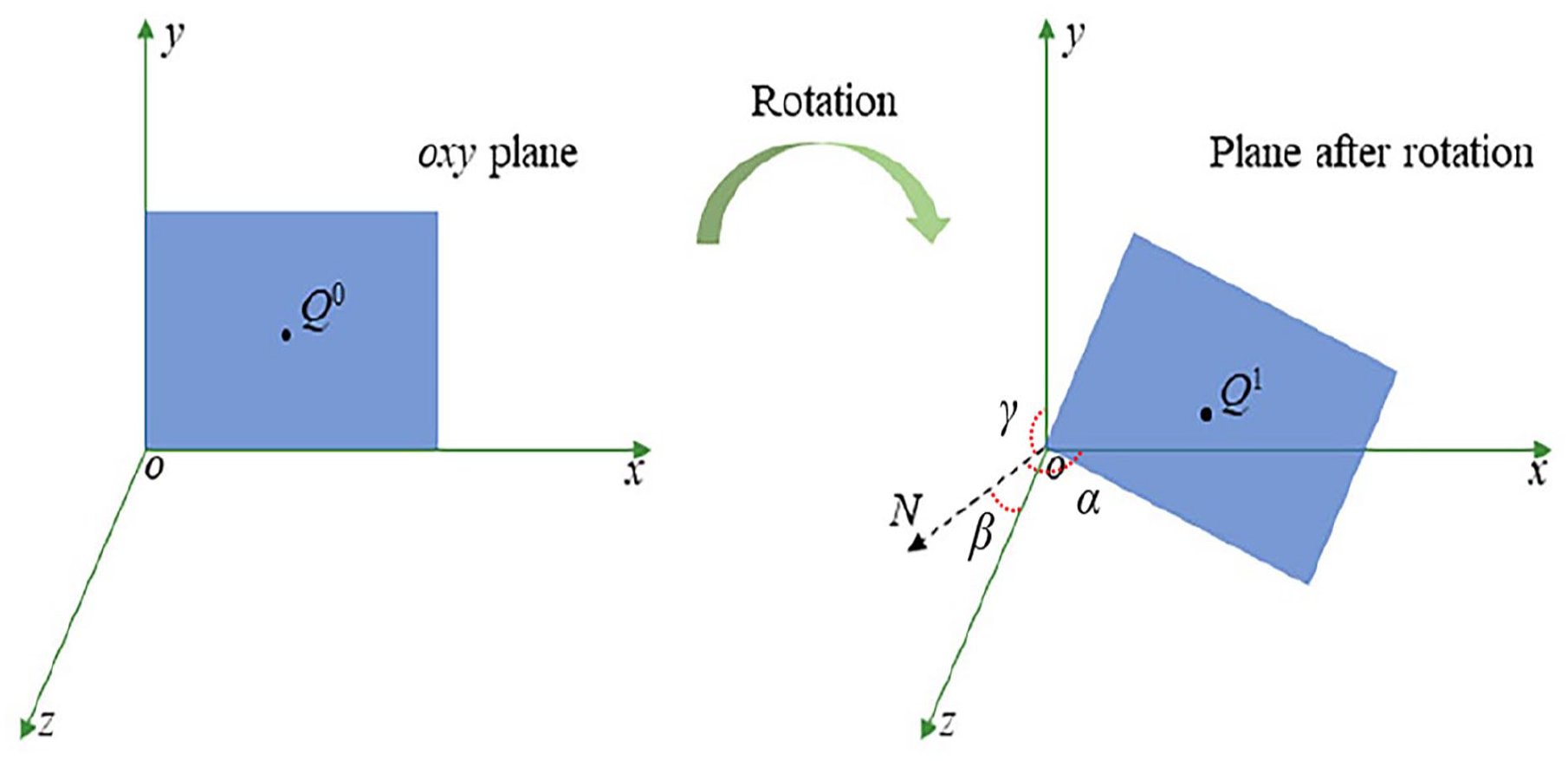
Schematic of plane rotation geometry.

Prior to the plane rotation, the coordinates of point Q⁰ are (x⁰, y⁰, z⁰). The coordinates of the corresponding point Q ¹ after rotation can then be expressed as ²⁵ :

$$\{\begin{array}{l}{x}^1=\frac{\cos \beta }{\sin \gamma }{x}^0+\cos \alpha \frac{\cos \gamma }{\sin \gamma }{y}^0+\cos \alpha z^0\\ y^1=-\frac{\cos \alpha }{\sin \gamma }{x}^0+\cos \beta \frac{\cos \gamma }{\sin \gamma }{y}^0+\cos \beta z^0\\ z^1=-\sin \gamma y^0+\cos \gamma z^0\end{array}$$

(8)

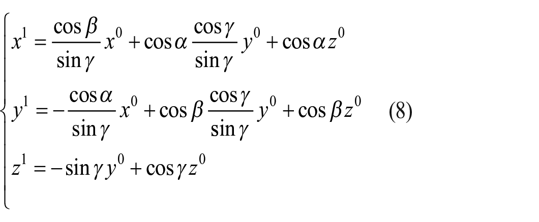
Introducing homogeneous coordinates, equation (8) is reformulated in matrix form as follows:

$$\left(\begin{array}{c}{x}^1\\ y^1\\ z^1\\ 1\end{array}\right)=\left(\begin{array}{cccc}\frac{\cos \beta }{\sin \gamma }& \cos \alpha \frac{\cos \gamma }{\sin \gamma }& \cos \alpha & 0\\ -\frac{\cos \alpha }{\sin \gamma }& \cos \beta \frac{\cos \gamma }{\sin \gamma }& \cos \beta & 0\\ 0& -\sin \gamma & \cos \gamma & 0\\ 0& 0& 0& 1\end{array}\right)\left(\begin{array}{c}{x}^0\\ y^0\\ z^0\\ 1\end{array}\right)$$

(9)

In equation (9), the fourth-order matrix represents the rotation matrix. To achieve the desired plane position, a translation transformation is also required. Figure 8 illustrates the schematic diagram of the plane’s translation transformation, where the normal vector of the plane remains unchanged after the translation.

Figure 8.

Schematic of plane translation geometry.

In Figure 8, point M corresponds to the translated point of point O. Let the translation vector be (x₀, y₀, z₀), then the coordinates of point M can be expressed as (x₀, y₀, z₀). By left-multiplying the fourth-order translation matrix, equation (9) is transformed to:

$$\left(\begin{array}{c}x\\ y\\ z\\ 1\end{array}\right)=\left(\begin{array}{cccc}1& 0& 0& x_0\\ 0& 1& 0& y_0\\ 0& 0& 1& z_0\\ 0& 0& 0& 1\end{array}\right)\left(\begin{array}{cccc}\frac{\cos \beta }{\sin \gamma }& \cos \alpha \frac{\cos \gamma }{\sin \gamma }& \cos \alpha & 0\\ -\frac{\cos \alpha }{\sin \gamma }& \cos \beta \frac{\cos \gamma }{\sin \gamma }& \cos \beta & 0\\ 0& -\sin \gamma & \cos \gamma & 0\\ 0& 0& 0& 1\end{array}\right)\left(\begin{array}{c}{x}^0\\ y^0\\ z^0\\ 1\end{array}\right)$$

(10)

Equation (10) provides the representation of the coordinates of the plane after rotation and translation, which includes the coordinates of the point Q, that is, (x, y, z). The parametric equation of the ellipse situated on the Oxy plane can be expressed as follows:

$$\{\begin{array}{l}{x}^0=a\cos \theta \\ y^0=b\sin \theta \\ z^0=0,0\le \theta \le 2\pi \end{array}$$

(11)

By substituting equation (11) into equation (10), the parametric equation of the spatial ellipse with a center at (x₀, y₀, z₀), a major semiaxis of length a, and a minor semiaxis of length b, situated on the plane cosα x+cosβ y +cosγ z = 0 (cos²α+cos²β+cos²γ = 1, cosγ ≠ 1) can be expressed as:

$$\{\begin{array}{l}x=x_0+\frac{\cos \beta }{\sin \gamma }a\cos \theta +\cos \alpha \frac{\cos \gamma }{\sin \gamma }b\sin \theta \\ y=y_0-\frac{\cos \alpha }{\sin \gamma }a\cos \theta +\cos \beta \frac{\cos \gamma }{\sin \gamma }b\sin \theta \\ z=z_0-\sin \gamma b\sin \theta ,0\le \theta \le 2\pi \end{array}$$

(12)

Continuing the generalization of equation (12), if the unit normal vectors (A, B, C) of a spatial ellipse are provided, along with the center (x₀, y₀, z₀), and the major and minor semiaxes a and b, respectively, the equation for the parameters of the spatial ellipse can be expressed as follows when A² + B² ≠ 0:

$$\{\begin{array}{l}x=x_0+\frac{B}{\sqrt{A^2+B^2}}a\cos \theta +\frac{AC}{\sqrt{A^2+B^2}}b\sin \theta \\ y=y_0-\frac{A}{\sqrt{A^2+B^2}}a\cos \theta +\frac{BC}{\sqrt{A^2+B^2}}b\sin \theta \\ z=z_0-\sqrt{A^2+B^2}b\sin \theta ,0\le \theta \le 2\pi \end{array}$$

(13)

When A² + B² = 0, the parametric equation of the spatial ellipse can be expressed as:

$$\{\begin{array}{l}x=x_0+a\cos \theta \\ y=y_0+b\sin \theta \\ z=z_0,0\le \theta \le 2\pi \end{array}$$

(14)

Flattening coefficient

During the weaving process of woven fabrics, factors such as tightness and weaving tension contribute to the compression of the yarns’ cross-sections. In this paper, we quantify this compression using the flattening coefficient, η. Figure 9 provides a schematic diagram illustrating the extent of yarn compression.

Figure 9.

Schematic diagram of yarn cross-section flattening.

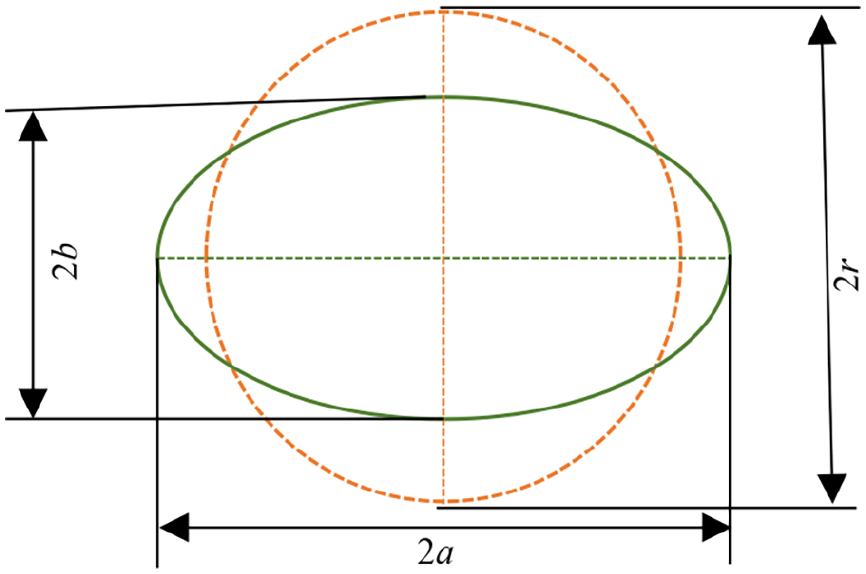
In Figure 9, r represents the unflattened radius of the yarn, while a and b are the major and minor semi-axes of the elliptical cross-section formed during interweaving, respectively. The value of b can be expressed as follows:

$$b=\eta \cdot r$$

(15)

Assuming the cross-sectional area remains constant during flattening, the value of a can be expressed as follows:

$$a=r^2/b=\frac{1}{\eta }\cdot r$$

(16)

Plain and floats structure

Yarns deform as they interact with other yarns during the weaving process, resulting in continuous changes in their cross-sectional shapes along their centerline trajectories. ²⁶ Figure 10 examines the cross-sectional shape of yarns, analyzing it from the perspective of fabric structure and the forces exerted at yarn contact points.

Figure 10.

Schematic diagram of force analysis of woven fabric.

In Figure 10, O represents a cross-section of the yarn. M₁M₂ denotes an intermediate cross-section of the warp located between two adjacent weft cross-sections (O₁ and O₂). O₄ through O_n indicate a warp floats structure, with O_middle positioned at the intermediate location of the floats. t_c refers to the thickness of the structural phases within the plain structure.

In the plain structure, the simplicity of the design allows us to assume that each interweaving point is subjected to a uniform force and experiences the same degree of compression. For simplification in our analysis, it is presumed that the warp and weft yarns contribute equally to the fabric’s structure, with identical diameters for both. In this context, the major and minor semi-axes of the yarn cross-section at the interweaving point in the plain structure are denoted by a₀ and b₀ respectively. The parameter t_c facilitates the expression of b₀ as follows:

$$b_0=\frac{1}{4}{t}_c$$

(17)

Based on equation (16), a₀ can be expressed as:

$$a_0=\frac{4r^2}{t_c}$$

(18)

The flattening coefficient of the yarn cross-section in this case is denoted as η₀, which can be expressed using equation (15):

$${\eta }_0=\frac{t_c}{4r}$$

(19)

Consider the plain structure’s interweaving intermediate point M₁M₂ cross-section with major and minor semi-axes denoted as a₁ and b₁, respectively. The value of b₁ can be computed using geometrical relationships. By applying the Pythagorean Theorem to calculate the length of segment O₁O₂ and determining the angle between ∠O₂O₁O₃ and ∠O₁O₂O₃, the calculation can be performed. Due to the complementary nature of these two angles, the lengths of O₁M₁ and O₂M₂ are equivalent. It is important to note that ∠O₂O₁O₃ is represented as φ. The length of O₁M₁ (which indicates the distance between a point on the circumference of the ellipse and the center of the ellipse) is then given by:

$$O_1{M}_1=\frac{a_0{b}_0}{\sqrt{a_0^2{\sin }^2\phi +b_0^2{\cos }^2\phi }}$$

(20)

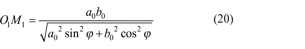
Subtracting 2O₁M₁ from O₁O₂ yields the length of M₁M₂, which represents the minor axis length of the intermediate section ellipse (2b₁). Let’s denote the intermediate cross-section flattening coefficient as η₁, which can be deduced from equation (15):

$${\eta }_1=\frac{M_1{M}_2}{2r}$$

(21)

To solve η₀ and η₁ in terms of a₀ and b₀, these aforementioned equations can be rewritten as follows:

$$\{\begin{array}{l}{\eta }_0=b_0/r\\ {\eta }_1=\frac{1}{2}\left(\sqrt{{(\Delta d_{weft})}^2+{(2b_0)}^2}-\frac{2a_0{b}_0}{\sqrt{a_0^2{\sin }^2\phi +b_0^2{\cos }^2\phi }}\right)/r\end{array}$$

(22)

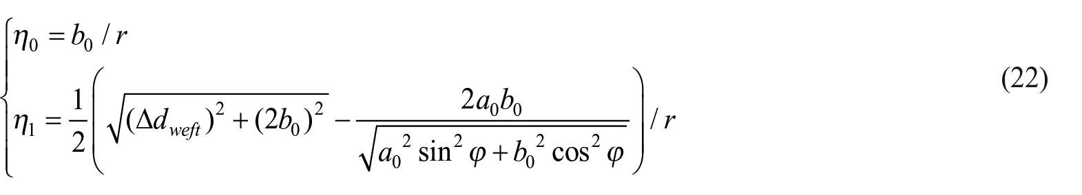
Equation (22) provides the flattening coefficient for both the weft yarns and the intermediate sections of the warp yarns. Considering the force analysis of the plain weave, it is reasonable to assume that the flattening coefficients at the interweaving points of both warp and weft yarns in the plain weave are all η₀, while the flattening coefficients of the intermediate sections are all η₁.

Within the floats structure (O₄~O_n) of the yarn section, compared to the plain structure section like O₀, there is reduced compression force on one or both sides, resulting in a corresponding reduction in the degree of flattening. Consequently, it is posited that the flattening coefficient of the cross-section within the floats is higher than that at the point of the plain weave, and this coefficient increases as one moves closer to the midpoint of the floats. In the scenario of infinitely long floats, the flattening coefficient of the middle-most section of the floats can be approximated as 1 (circular cross section in the initial state). Thus, the depicted floats should demonstrate symmetry and a subtly elevated visual effect.

The degree of flattening of the yarn cross-section under the floats is more complex than in the plain weave. To simplify representation, the two types of structures are consolidated. The flattening coefficient at the interweaving point in both structures is represented by η_z, as calculated in equation (23):

$${\eta }_z=b_0/r+f(k)k\ge 1$$

(23)

In this context, k represents the length of the floats, indicating the number of yarns beneath them, while f is a user-defined exponential function. When k equals 1, it denotes a plain structure at this point. Consequently, when k equals 1, f(1) equals 0, ensuring that the upper limit for η_z does not exceed 1.

The discussion of η_m for the intermediate cross-section of the yarn can be approached in two scenarios:

• 1) When considering an adjacent interlacing point forming a plain weave structure, the computation of η_m, representing the flattening coefficient of the intermediate cross-section at the interweave point within the plain weave (η₁), is illustrated in equation (22);

• 2) Within the floats, the flattening coefficients η_z of the interweaves before and after were summed for averaging.

After calculating the flattening coefficients for both the interwoven and intermediate cross-sections using the model described, it is observed that the flattening coefficients of the yarn cross-sections exhibit a consistent trend, either increasing or decreasing linearly.

Leno structure

The variable coefficient elliptic cross-section model previously discussed effectively simulates most single-ply woven fabric weaves. However, modifications are necessary to accurately represent the distinct structure of leno fabrics. Figure 11 illustrates the interweaving of warp and weft yarns within the leno structure, showing two entwined warp yarns, labeled Warp₀ and Warp₁. Points W₀ and W₂ represent the intersections where the weft yarns interweave with the warp yarns, while W₁ denotes an intermediate point in the weft interweaving process. Notably, labels E and F indicate the compressive forces exerted on the weft yarns following the entwining of the warp yarns.

Figure 11.

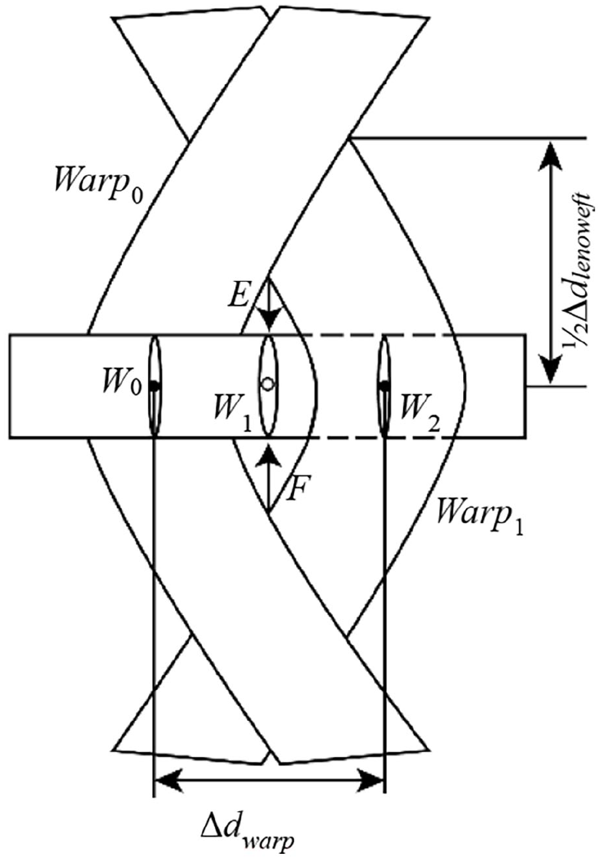
Analysis of warp and weft interweave of leno structure.

The leno structure creates a narrow aperture as the warp yarns intertwine. In cases where the weft yarns are woven through this aperture without contacting the warp yarn cross-section, it becomes crucial to recalibrate the flattening coefficient at the intermediate weft interweave point (W₁).

Upon kinking the warp yarns together, two equivalent compressive forces, denoted as E and F, materialize on the weft yarns interwoven within the apertures. A vertical cross-section taken at the weft yarn data points is presumed to exhibit an identical flattening configuration at positions W₀ and W₂, akin to that observed at the plain weave interlacing point. Consequently, the flattening coefficient at these locations remains consistent and is represented by η₀. W₁ is influenced by forces both above and below, denoted as E and F. As a result, the long axis of the elliptical cross-section undergoes compression and contraction (leading to a decrease in the value of a), while the short axis expands proportionally (resulting in an increase in the value of b), all while maintaining a constant area. The flattening coefficient at W₁ is denoted as η₂, and η₂ > η₀ due to the increase in the b value. For the middle section of the yarn, η_m is further extended to be discussed in three cases:

• 1) When considering an adjacent interlacing point forming a plain weave structure, the computation of η_m, representing the flattening coefficient of the intermediate cross-section at the interweave point within the plain weave (η₁), is illustrated in equation (22);

• 2) Within the floats, the flattening coefficients η_z of the interweaves before and after were summed for averaging;

• 3) Within the holes created by the entwining of warp yarns in the leno structure, the value of η_m is η₂.

After defining the value of η₂, the minor and major semi-axes of the cross-section are calculated using equations (15) and (16) respectively.

Multifilament model

Multifilament yarn is composed of either untwisted or twisted bundles of monofilaments fused together. This paper utilizes multifilament yarns as the warp and weft model in woven fabric simulations, aiming to accurately capture the fabric’s textural effects at the fiber level.

Algorithm for equalizing elliptic circumference

Assuming a uniform distribution of surface layer monofilaments within each multifilament cross-section. This arrangement facilitates the formation of a multifilament surface layer structure. For illustration, Figure 12 depicts a model of a multifilament cross-section, where the surface layer consists of n monofilaments. In this model, E_j represents the serial number of the multifilament cross-section (j = 1. . .8), and C_i denotes the serial number of each monofilament within the structure (i = 1. . .n).

Figure 12.

Multifilament cross-sectional model.

The position of each monofilament’s center within the cross-section is determined by dividing the ellipse’s perimeter equally. However, calculating the perimeter and arc length of an ellipse typically involves elliptic integrals of the second kind or infinite series, complicating the acquisition of an exact solution. To address this, the perimeter of the ellipse, denoted as L, is approximated using Ramanujan’s formula ²⁷ :

$$L=\pi (a+b)\left[1+\frac{3h^2}{10+\sqrt{4-3h^2}}\right]$$

(24)

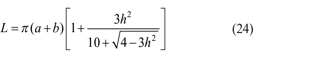
In equation (24): where h = (a − b)/( a + b), a and b represent the major and minor semi-axes of the ellipse, respectively. The circumference L is computed, and subsequently, the arc length S of the ellipse is evaluated using the approximate Equation:

$$S=\frac{L}{2\pi }\theta -\frac{\sin (2\theta )}{4\pi {\left(\frac{{\sin }^2(\theta )}{{(2a\pi -L)}^{13/3}}+\frac{{\cos }^2(\theta )}{{(L-2b\pi )}^{13/3}}\right)}^{3/13}}$$

(25)

In equation (25): where θ represents the eccentric angle of the ellipse. Utilizing equations (24) and (25), the ellipse circumference can be divided into equal segments programmatically. Figure 13 displays the pseudo-code algorithm designed for calculating equidistant points along an elliptical circumference.

Figure 13.

Pseudocode algorithm for dividing the circumference of an ellipse evenly.

Calculation of multifilament twist

The algorithm for evenly dividing the circumference of an ellipse is primarily used to generate monofilaments on the surface of a multifilament. To account for the twisting effect of the multifilament, a modification has been applied to the elliptic perimeter equalization algorithm. This study uses the twist angle, defined as the angle between a surface monofilament and the yarn axis, to quantify the degree of multifilament twisting. Figure 14 illustrates the spatial relationship between the trajectory direction of the surface monofilament and the twist angle β. In this figure, EE′ represents the axial line of the multifilament, h indicates the lay length in millimeters (mm), and L denotes the perimeter of the cross-section, also in millimeters (mm).

Figure 14.

Monofilament trajectory and twist angle.

Figure 15 illustrates variation of the peripheral vertices of the multifilament ellipse in both radial and axial directions after the addition of the twist angle parameter. In this figure, C (i = 1,2,3,4) _i represents the center position of the monofilament in the cross section of the multifilament when it is untwisted, and C_i^′ (i = 1,2,3,4) represents the center position of the monofilament after twisting.

Figure 15.

Schematic illustration of elliptical perimeter vertex variation: (a) radial direction and (b) axial direction.

In Figure 15, β represents the twist angle of the multifilament, φ denotes the initial angle (rotation angle) of the monofilament offset influenced by the twist angle β, and α corresponds to the centrifugal angle associated with φ. The relationship between these two angles is as follows:

$$\tan \alpha =\tan \phi \cdot \frac{a}{b}$$

(26)

Where L_a and L_a+1 represent two adjacent cross-sections, and l is the distance between L_a and L_a+1. Therefore, the following relationships hold:

$$S=\tan \beta \cdot l$$

(27)

Substitute θ in equation (25) with α, and employ algorithmic steps similar to those depicted in Figure 13 to iteratively approximate the value of S in order to solve for α, which represents the initial centrifugal angle θ. Since the arc length of an ellipse cannot be evenly divided by the central angle, α is only the offset angle for the first point on the circumference. To achieve an accurate twist angle and even division of the ellipse circumference, modifications were made to the ellipse division algorithm. Before twisting, the value of S is calculated using equation (25) and is essentially S(θ), with the initial eccentric angle set to 0. After twisting, the initial eccentric angle changes to α. Therefore, during twisting, S can be expressed as:

$$S=S\left(\theta +\alpha \right)-S\left(\theta \right)$$

(28)

Experimental results and discussion

Simulation results with different parameters

To validate the accuracy of the aforementioned mathematical model, simulations of multifilaments and fabric weaves were conducted using C# and OpenGL. Discussions were carried out on key parameters, including fabric count, the flattening state of the cross-section, the number of monofilaments in the surface arrangement of multifilaments, and the twist.

Fabric count

In Section 2.1, the yarn spatial trajectory model introduces parameters related to fabric count, namely Δd_warp, Δd_weft, and Δd_lenoweft. Figure 16 illustrates the simulation results of the same fabric structure under three different fabric count parameters.

Figure 16.

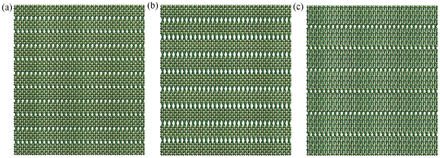
Simulation of leno fabrics at different fabric counts: (a) Δd_warp = Δd_weft = 0.5·Δd_lenoweft, (b) Δd_warp = Δd_weft = 0.3·Δd_lenoweft, and (c) Δd_warp = 0.5·Δd_weft = 0.5·Δd_lenoweft.

The leno fabric depicted in Figure 16(a) are composed of 60 warp yarns and 55 weft yarns. If we take Figure 16(a) as the reference, in Figure 16(c), the value of Δd_weft is exactly twice that of (a), resulting in a reduction of 20 yarns in the number of weft yarns in the same fabric dimensions. In Figure 16(b), although Δd_warp and Δd_weft are equivalent to those in (a), a larger value of Δd_lenoweft results in further elongation of the hexagonal yarn holes on the fabric surface in the warp direction. In the same dimensions, the number of weft yarns is reduced by 10. Through the adjustment of the aforementioned three parameters and the transformation of geometric relationships, various fabric counts and distinct hexagonal yarn apertures can be obtained.

Flattening state of the cross-section

In Section 2.2, the variable coefficient elliptic cross-section model employs the flattening coefficient η to represent the degree of yarn flattening. The flattening degree of yarns varies across different fabric structures. Figure 17 illustrates three fabric structures simulated based on this model. At the interweaving points of plain weave, where the forces are most concentrated, the degree of yarn deformation is maximized. The cross-sectional deformation of the interweaving points within the floats is characterized by a gradual reduction in deformation due to the decrease in compressive forces. In the leno structure, the cross-sectional profile of the weft yarns within the woven-in holes also demonstrates a distinct contraction. In this simulation, η_z (the flattening coefficient at the interlacing points) is 0.7 for plain weave, 0.82 for twill weave, and identical to plain weave for leno weave, η₂(the flattening coefficient for the cross-sectional profile of the weft yarns within the woven-in holes) is 0.9.

Figure 17.

Simulation of different fabric structures: (a) plain structure, (b) twill structure, and (c) leno structure.

Yarn count and twist

In Section 2.3, num and β are two parameters representing the number of monofilaments in the multifilament surface and the twist of the multifilament, respectively. The value of num is calculated by dividing the ellipse perimeter L by the monofilament diameter, and then taking the lower bound of the result. When the monofilament fineness is consistent, the value of num represents the size of the yarn count. Figure 18(a) shows the simulated effects of different yarn counts under various num values. The simulated effects of varying yarn twists at different twist angles (β) are shown in Figure 18(b) (considering β = 0 as a special case of twisted multifilament).

Figure 18.

Simulation effects of multifilament under different parameters: (a) num and (b) β.

The fabric simulation results for two yarn models, the curved cylinder, and num = 10, β = 15° twisted multifilaments, are illustrated in Figure 19. Compared to the smooth curved cylinder, the multifilament model, due to features such as the twist and the twist direction of monofilaments on the surface, simulates the fabric with enhanced detail, providing a representation that is more faithful to real-world textiles.

Figure 19.

Comparison of simulation results of multifilaments and curved columns: (a) rhombic twill weave, (b) leno weave, and (c) plain-leno weave.

Comparison of collision detection algorithms

Figure 20 illustrates the simulation results of plain and 2/2 twill weaves, where h_T represents the yarn waviness. Under the same yarn waviness conditions, compared to the circular fixed cross-section, the model established in this paper can calculate the cross-sectional shape based on geometric relationships, effectively reducing yarn penetration. From Figure 20, it can be observed that the cross-sections of yarns in the fabric continuously change. At the plain weave intersection points, where the force is the greatest, the degree of deformation is the highest. In contrast, the deformation of the intersection points within the floats is more gradual due to the reduction of squeezing pressure, which is consistent with actual conditions.

Figure 20.

Diagram of plain and twill weave simulation: (a) plain weave and (b) twill weave.

If a segment of multifilament path consists of 200 nodes, with 10 monofilaments on the surface layer, and each monofilament section has 10 vertices, Table 1 shows the number of triangular facets and time complexity involved in the operation of the proposed algorithm compared to traditional collision detection algorithms. Compared to traditional collision detection algorithms such as ray detection and hierarchical bounding box, the interlacing model established in this paper avoids complex triangular facet intersection operations, saving program execution time and improving algorithm efficiency. Additionally, the geometric approach to handling yarn penetration issues in woven fabrics ensures both efficiency and theoretical accuracy, as the warp and weft yarn systems have their inherent interlacing rules.

Table 1.

Comparative analysis of collision algorithms.

Algorithm	Number of triangular facets	Time complexity
Ray detection	39,800	O(n2)
Hierarchical bounding box	5800	O(n log n)
This paper	/	O(n)

The hierarchical bounding box algorithm is an optimization based on ray detection, with the number of nodes in the final level bounding box for yarn segments set to 30.

Comparison with actual leno structures

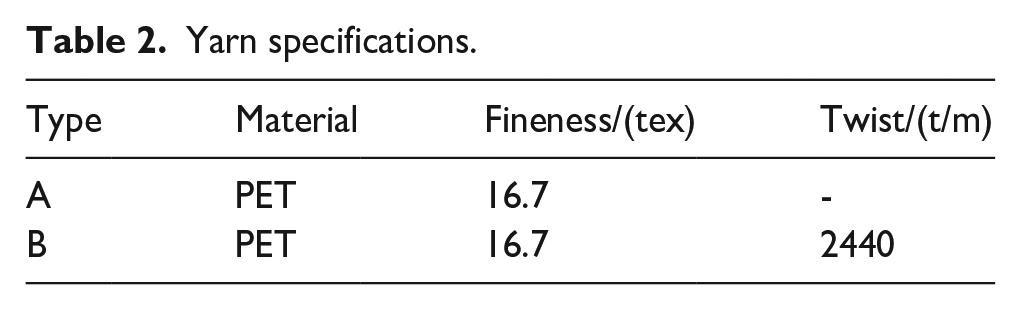
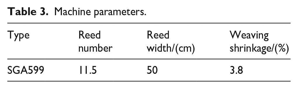
Three leno structures were woven on a sample loom to verify the accuracy of the algorithms in this paper. Some yarn parameters such as yarn material, fineness and twist are designed and the specific data are shown in Table 2. We used two types of yarns (A and B), that is, untwisted and twisted multifilaments, respectively. The samples are woven by machine SGA599, and the relevant machine parameters are shown in Table 3.

Table 2.

Yarn specifications.

Type	Material	Fineness/(tex)	Twist/(t/m)
A	PET	16.7	-
B	PET	16.7	2440

Table 3.

Machine parameters.

Type	Reed number	Reed width/(cm)	Weaving shrinkage/(%)
SGA599	11.5	50	3.8

The real product picture and simulation result is illustrated in Figure 21. Figure 21(a)–(c) depict the comparison of untwisted multifilaments, while Figure 21(d)–(f) show the corresponding structures with twisted multifilaments. The simulation results indicate that the hexagonal holes on the surface of the simulated fabric are well-defined and rounded, aligning closely with the features of the actual fabric. The real fabric confirms that the weft yarns undergo a reduction in cross-section as they traverse the openings created by the warp yarns, a phenomenon attributed to the compression exerted by adjacent warp yarns. This aligns with the principles of the variable coefficient elliptic cross-section model proposed in this paper. The multifilament model adds textural features to the simulated fabric, making the simulation more realistic.

Figure 21.

Validation of simulation algorithm: (a) Type 1, (b) Type 2, (c) Type 3, (d) Type 1′, (e) Type 2′, and (f) Type 3′.

Conclusion

This paper introduces a three-dimensional simulation algorithm for leno fabrics that thoroughly addresses essential aspects of fabric simulation, from spatial structure to yarn cross-sections and surface textures. Comparative analysis with real samples confirms the algorithm’s capacity to precisely simulate the spatial structure and detailed surface texture of fabrics, meeting the anticipated outcomes. This algorithm is readily integrable into computer-aided design systems, significantly reducing the proofing cycle and boosting the production efficiency of leno fabrics. The successful simulation results also provide substantial insights beneficial for both designing and teaching leno fabrics.

The methodological approach of deriving parametric equations for spatial ellipses shows promise for broader applications across various plane geometries, advancing the field of fiber simulation. However, that the current multifilament model focuses solely on surface monofilaments and omits the complex internal monofilament interactions. Future research will address this gap by developing an advanced fiber transfer algorithm that integrates fiber radial distribution parameters, aiming for a more comprehensive understanding and representation of fiber interactions within fabrics.