Sage Journals: Discover world-class research

Abstract

Molded pulp products can improve the utilization of recycled paper by achieving close to zero waste emission and a 100% recycling rate, while satisfying the national goals for recycled packaging materials of various countries. Molded pulp products are often designed using finite-element simulations to optimize their performance, which requires the input of accurate material properties. However, studies on the constitutive model, an essential factor related to material properties, are still rare. This study investigated the mechanical behavior of the molded pulp material to simplify the parameters and improve the accuracy of the constitutive model. The fiber distribution and connection within the molded pulp material were investigated; treating the pores of the molded pulp as a virtual material enhances the meso-mechanical model and gives a transversely isotropic constitutive model. The elastic modulus in the thickness direction was calculated as 1.5997 MPa, and the experimentally measured value is 1.5368 MPa. The error of proposed model is 4.1%, but significantly smaller than treating molded pulp as an isotropic material, the error of which is ~80 times larger of experimental result.

Keywords

Molded pulp transverse isotropic elastic modulus meso-mechanical model

Introduction

Molded pulp (or molded fiber) from recycled paper has been used for decades. Before environmental protection became mainstream, molded pulp was mainly used for agricultural product trays. With the growing recycling industry, molded pulp has found new applications as the inner packaging for electronic components and heavy machine parts. There has been a significant increase in the use of molded pulp in China, especially for inner packaging. Governments of various countries have also developed policies to encourage consumers and producers to use recycled packaging materials. For example, the EU Council published the goal to recycle 70% of packaging waste by 2018 and 75% of paper and cardboard by 2025.¹ Similarly, Japan has formulated a series of waste recycling and management laws.² China implemented the Circular Economy Promotion Law in 2009 to increase the efficiency of resource use and protect the environment.² The application of molded pulp in packaging material provides an excellent scenario for implementing these regulations and policies. Molded pulp can effectively improve the utilization of recycled paper and packaging materials by achieving close to zero waste emission and a nearly 100% recycling rate.

The 3D structural design of molded pulp products (MPPs) is being thoroughly researched. For example, a relationship between the shape of the molded pulp structure and its dynamic strength was identified.³ A previous study calculated the relationship between cushioning performance and maximum stress by equivalent region theory,⁴ while the influence of the MPM bucket unit on the cushion performance of MPPs was investigated using the finite element method.⁵ Furthermore, a device was developed for measuring the torsional stiffness of various MPPs.⁶

Another critical research trend is investigating the material behavior of molded pulp. The tensile and compressive elastic modulus of molded pulp were measured as 225 and 130 N/mm², respectively.⁷ Furthermore, the digital image correlation method was used to measure the Poisson’s ratio of molded pulp materials (MPMs), which gave results consistent with microscopy results.⁸ Later, the same group tested the tensile properties of MPM under different loading conditions following the ISO1924-2 standard.⁹ The results showed that the elastic modulus increased by 10% when the loading rate increased from 1 to 150 mm/min. In addition, MPM was evaluated via tensile tests, and the results were applied to a cushioning structural design.¹⁰ Other studies improved the empirical uniaxial-compression nonlinear equation for MPMs and found that the microscale deformation of molded pulp was non-uniform.^11–14 Furthermore, compression analysis of large MPPs using isotropic material method for MPM was performed,¹⁵ along with measurements of the strength and porosity of paper.^16,17 Other studies measured the uniaxial tensile properties and elastic modulus of molded pulp made from three kinds of non-wood pulp and their mixed pulp.^18,19 All these researchers worked on sheet-scale samples²⁰ and did not consider the fiber network scale.

The fiber network must be considered to provide detailed information about MPMs. Alava and Niskanen first showed that the fiber distribution of paper is random in the paper plane and laminated in the vertical plane by X-ray and scanning electron microscopy (SEM) methods.²¹ Subsequently, various research groups observed the same fiber microstructure in molded pulp by SEM.^22–24 A continuum model at the mesoscale level was used to study the effect of the uneven fiber distribution on the local strain field,²⁴ which showed that the inhomogeneous density distribution has the most significant effect. These previous studies only observed the fiber network of MPMs and did not apply the data to constitutive modeling of the material. In general, isotropic models^5,10,15,22 are used to simulate and analyze MPMs, which do not consider the layers and connections between them.

In this study, the fiber network of MPMs was studied by field-emission scanning electron microscopy (FSEM), and the distribution of fibers in three directions at the fiber scale was considered. A modified meso-mechanical model is proposed using the meso-mechanics theory to treat pores as a virtual material. Finally, the transverse isotropic model parameters were identified by compression and porosity tests, and use of the digital image correlation method. This method enables porosity and morphological testing to be completed before mass production, then a simple uniaxial compression test can be predict the normal and shear elastic modulus of the material other than the testing direction.

Constitutive model of molded pulp materials

This study used MPPs provided by Wuhan Peng Huan Packaging Co., Ltd. This company uses an assembly production line to produce MPPs similar to that used for making paper. First, in the pulp-beater stage, the recycled paper is degraded into fibers with water to make a pulp. Second, the pulp and water are pumped into a pulp tank with a particular fiber content by a spiral pump to adjust the fiber–water ratio. Third, vacuum adsorption is applied to the pulp to shape it into a 3D product. Finally, the MPP is carried through a drying oven on a conveyor belt.

Because MPPs are made from paper pulp, the main structure of the MPM is wood fibers. The different fiber lengths produce different fiber distributions when the fibers are randomly oriented.²⁵ If the fiber length is much smaller than the thickness of the part, the fibers will be truly randomly oriented, and the material will have isotropic properties in 3D. However, if the fiber length is greater than the thickness of the part, the fiber orientation is only randomly distributed within the plane, and the material is transversely isotropic. This characteristic is highly significant in the construction of a constitutive model.

The morphological features of the paper fibers depend on the tree species. Thus, a fiber length distribution of ~900–1600 μm and fiber aspect ratio of 35–45 are typical of industrial raw materials.²⁶ FSEM is required to quantify the fiber length and width and determine the fiber distribution of a sample. The geometry of the MPM studied here is defined by the schematic in Figure 1. The surfaces parallel to the 0xy plane are called surface planes, and the planes normal to the 0 z axis are called cross-sectional planes. These definitions will be used throughout the paper.

Figure 1.

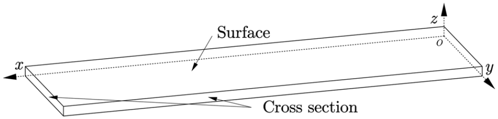
Definition of the geometry of the studied MPM.

Fiber distribution of molded pulp

The fiber distribution in the studied MPM was investigated by FSEM, as shown in Figure 2. Figure 2(a) shows the surface plane, where the fibers are randomly oriented in the plane and overlap. Figure 2(b) shows the significant horizontal distribution of the fibers in a cross-sectional plane. These images show that the fiber length in this specimen was >0.5 mm and the observed specimen is ~1.3 mm. Based on the results presented in Figure 2, it can be observed that the fiber in the cross-sectional plane only presents the distribution parallel to the surface plane, and the length of the fibers is also greater than the macroscopic thickness of the MPM, meets the definition of the fiber distribution theory of non-continuum fiber reinforced materials.²⁵

Figure 2.

(a) Surface and (b) cross-sectional of the fiber distribution of the molded pulp sample.

Based on the fiber distribution, it is reasonable to describe the constitutive model of the MPM as transversely isotropic. According to Hooke’s law, there is a proportional relationship between strain and stress within the linear-elastic region. Equation (1) describes the relationship transformed into a cartesian system.

{ε} = [c] {σ}

(1)

In this equation, {ε} is strain, {σ} is stress, and [c] is the flexibility matrix. According to the axis symmetry of the transversely isotropic system, only five independent variables are specified for [c]:

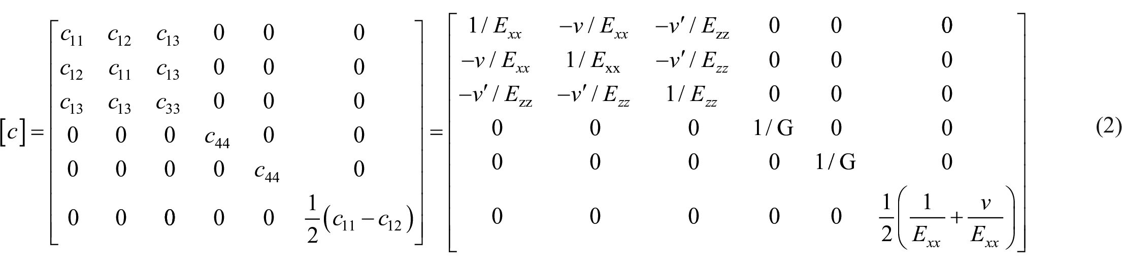
[c] = [\begin{matrix} c_{11} & c_{12} & c_{13} & 0 & 0 & 0 \\ c_{12} & c_{11} & c_{13} & 0 & 0 & 0 \\ c_{13} & c_{13} & c_{33} & 0 & 0 & 0 \\ 0 & 0 & 0 & c_{44} & 0 & 0 \\ 0 & 0 & 0 & 0 & c_{44} & 0 \\ 0 & 0 & 0 & 0 & 0 & \frac{1}{2} (c_{11} - c_{12}) \end{matrix}] = [\begin{matrix} 1 / E_{x x} & - v / E_{x x} & - v^{'} / E_{zz} & 0 & 0 & 0 \\ - v / E_{x x} & 1 / E_{xx} & - v^{'} / E_{z z} & 0 & 0 & 0 \\ - v^{'} / E_{zz} & - v^{'} / E_{z z} & 1 / E_{z z} & 0 & 0 & 0 \\ 0 & 0 & 0 & 1 / G & 0 & 0 \\ 0 & 0 & 0 & 0 & 1 / G & 0 \\ 0 & 0 & 0 & 0 & 0 & \frac{1}{2} (\frac{1}{E_{x x}} + \frac{v}{E_{x x}}) \end{matrix}]

(2)

Here, E_xx is the elastic modulus of the x- and y-axes, E_zz is the elastic modulus along the z-axis, ν is Poisson’s ratio of the surface plane, ν′ is Poisson’s ratio of the cross section plane, and G is the shear modulus of the x-axis to the z-axis and the y-axis to the z-axis.

Correlation between independent variables of the constitutive model based on meso-structural mechanics

For accurate modeling, MPPs are made from different raw materials, the different MPPs must be measured separately along normal to surface and cross section plane moduli and surface plane edge to surface plane shear.²⁷ The material properties need to be clarified before the design and modeling of MPPs. The fiber distribution and porosity of MPPs are constant if they are fabricated using the same production process and parameters. Therefore, the number of measurements can be reduced by using only tensile or compression test results and calculating the others. This can help save time and reduce costs related to sampling and testing.

The model is derived based on the following assumptions:

(1) When a simple external load is applied to a porous material, only the corresponding internal stress is generated, and other internal stresses are zero.

(2) The axial strain produced by a fiber and pore is equal under axial load.

(3) The stress produced by a pore is zero under simple external load.

(4) As a virtual material, the elastic modulus of the pore is close to zero but not equal to zero.

(5) The fiber material is isotropic, and its Poisson’s ratio is equal to that of the composite material in the isotropic plane.

A typical cross-sectional plane pore morphology of MPM is shown in Figure 2(a). The interval between adjacent fibers (diagonal lines) is the main feature of the fiber distribution. A simplified unit cell with dimensions of a × a is defined, with a pore in its center. In Figure 2(b), the pore is modeled by an ellipse, where the major axis (a_e0) and minor axis (b_e0) of the ellipse and the angle (θ) between the major axis and the x-axis are labeled. The ratio between the major and minor axis lengths is used to define a rectangle with long (a_p) and short (b_p) edges, with exactly the same area as the original irregular pore. Then, meso-structural mechanics theory is used to calculate the elastic modulus of both sides of the pore.

Figure 3(b) shows the ellipse used to fit the pore edge, which is defined by the major and minor axis of the ellipse (a_e0 and b_e0, respectively). These two parameters are adjusted by an amplification coefficient of the ellipse k₀ from the original ellipse fit result of major and minor axis (a_e and b_e, respectively) to set the ellipse area to equal that of the original pore.

\begin{matrix} a_{e 0} = a_{e} * k_{0} \\ b_{e 0} = b_{e} * k_{0} \end{matrix}

(3)

Figure 3.

Schematics of the unit cells defined to characterize a pore in the MPM: (a) original MPM pore morphology and converted to (b) ellipse modeled pore, then converted to (c) rectangle pore. (d) Unit cell area partition and (e) splitting to three parts.

Figure 3(c) defines the rectangle as a simplified form of the ellipse to calculate the unit cell porosity V_p:

V_{p} = \frac{a_{p} b_{p}}{a^{2}}

(4)

Here, a_p = a_e*cosθ and b_p = b_e*cosθ. Then, a ratio between the pore width and height (k) is defined as follows, and is used to transform equation (4):

\begin{matrix} \frac{b_{e 0}}{a_{e 0}} = \frac{b_{e}}{a_{e}} = \frac{b_{p}}{a_{p}} = k \\ V_{p} = \frac{a_{p} b_{p}}{a a} = k {(\frac{a_{p}}{a})}^{2} = \frac{1}{k} {(\frac{b_{p}}{a})}^{2} \end{matrix}

(5)

Subsequently, the porosity (V_p), and cell length relationships are found as follows:

\begin{array}{l} \frac{a_{p}}{a} = \sqrt{\frac{V_{p}}{k}}, \frac{a_{f}}{a} = 1 - \sqrt{\frac{V_{p}}{k}}, \\ \frac{b_{p}}{a} = \sqrt{k V_{p}}, \frac{b_{f}}{a} = 1 - \sqrt{k V_{p}} \end{array}

(6)

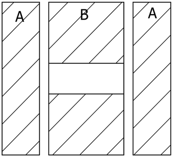
Considering a load parallel to the 0x axis applied to this unit cell, the cell is sectioned by horizontal lines to denote the area in which the pore is contained (Figure 3(d)). Then, the cell is divided into three parts, as shown in Figure 3(e). In the typical cell, the two parts labeled A contain only fibers, while part B contains fibers and a pore. According to the mixed model hypothesis, the fiber and pore should have equal internal stress. This relationship for the Ox axis can be written as follows:

\frac{1}{E_{B x x}} = \frac{a_{f} / a}{E_{f}} + σ \frac{a_{p} / a}{E_{p}}

(7)

Here, E_Bxx is the elastic modulus of area B, E_f is the elastic modulus of the fiber, E_p is the elastic modulus of the virtual pore material, and $a_{f} = a - a_{p}$ is the fiber area fraction of area B. We treat area B as a new material to analyze the unit cell. The load along the 0x axis induces equal strains in areas A and B, as follows:

E_{x x} = E_{B x x} \frac{b_{p}}{a} + E_{f} \frac{b_{f}}{a}

(8)

Here, E_xx is the elastic modulus of the entire unit cell along the 0x axis, and $b_{f} = a - b_{p}$ is the area fraction of area B. By substituting equation (6) into equation (8), E_Bxx can be described by the following equation:

E_{B x x} = \frac{E_{f} E_{p}}{E_{p} (1 - \sqrt{V_{p} / k}) + σ E_{f} \sqrt{V_{p} / k}}

(9)

Then, equation (8) can be rewritten as follows:

E_{x x} = E_{f} (\sqrt{k V_{p}} (\frac{E_{p}}{E_{p} (1 - \sqrt{V_{p} / k}) + σ E_{f} \sqrt{V_{p} / k}} - 1) + 1)

(10)

Assuming E_h→0 and the inner stress produced by the pore $σ = σ_{p} / σ_{B} = 0$ , equation (10) becomes

E_{x x} = E_{f} (1 - \sqrt{k V_{p}})

(11)

Considering the load along the 0z axis, Figure 4 shows a vertical method similar to that shown in Figure 3(e). The analysis of load along the 0z axis was similar to that for the 0x axis. The E_Bzz and E_zz values are defined below:

\frac{1}{E_{Bzz}} = \frac{b_{f} / a}{E_{f}} + σ^{'} \frac{b_{p} / a}{E_{p}}

(12)

E_{z z} = E_{B z z} \frac{a_{p}}{a} + E_{f} \frac{a_{f}}{a}

(13)

Figure 4.

Vertical method for defining the unit cell with a pore.

By substituting equation (6) into equation (12), E_Bzz is written as follows:

E_{Bzz} = \frac{E_{f} E_{p}}{E_{p} (1 - \sqrt{k V_{p}}) + σ^{'} E_{f} \sqrt{k V_{p}}}

(14)

By substituting equation (6) and (13) into (14), E_zz becomes

E_{z z} = E_{f} ((\sqrt{V_{p} / k}) (\frac{E_{p}}{E_{p} (1 - \sqrt{k V_{p}}) + σ^{'} E_{f} \sqrt{k V_{p}}} - 1) + 1)

(15)

Again, assuming E_p→0 and the inner stress produced by the pore σ′=σ′_p⁄σ′_B = 0, we obtain

E_{z z} = E_{f} (1 - \sqrt{V_{p} / k})

(16)

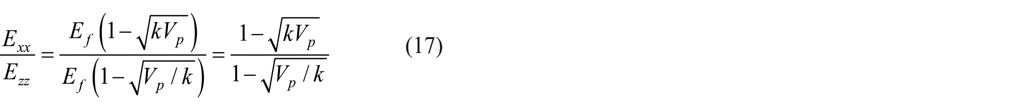
Then, the elastic modulus ratio between the 0x and 0z axes is obtained by dividing equation (11) by (16) to obtain

\frac{E_{x x}}{E_{z z}} = \frac{E_{f} (1 - \sqrt{k V_{p}})}{E_{f} (1 - \sqrt{V_{p} / k})} = \frac{1 - \sqrt{k V_{p}}}{1 - \sqrt{V_{p} / k}}

(17)

Similar to the elastic modulus analysis, the shear modulus was obtained as follows. In equation (18) G_B is the elastic modulus of area B, and G is the overall elastic modulus in equation (19).

\frac{1}{G_{B}} = \frac{a_{f} / a}{G_{f}} + τ \frac{a_{p} / a}{G_{p}}

(18)

Here τ = τ_p ⁄ τ_B, τ_p = 0 is the shear stress produced by the pore, τ_B is the overall shear stress of area B, G_f is the shear modulus of fiber, and G_p→0 is the shear modulus of the pore.

G = G_{B} \frac{b_{p}}{a} + G_{f} \frac{b_{f}}{a}

(19)

By substituting equation (6) into (18), G_B is written as follows:

G_{B} = \frac{G_{f} G_{p}}{G_{p} (1 - \sqrt{V_{p} / k}) + τ G_{f} \sqrt{V_{p} / k}}

(20)

Substituting equations (6) and (20) into (19), G becomes

\begin{array}{l} G = G_{B} \frac{b_{p}}{a} + G_{f} \frac{b_{f}}{a} \\ = G_{f} (\sqrt{k V_{p}} (\frac{G_{p}}{G_{p} (1 - \sqrt{V_{p} / k}) + τ G_{f} \sqrt{V_{p} / k}} - 1) + 1) \end{array}

(21)

Assuming G_p→0 and τ = τ_p⁄τ_B = 0 the following equation is obtained.

G = G_{f} (1 - \sqrt{k V_{p}})

(22)

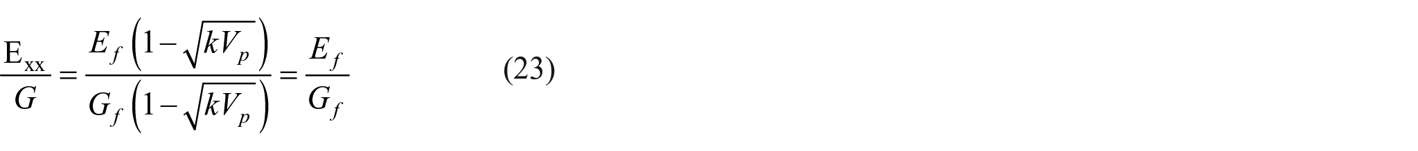
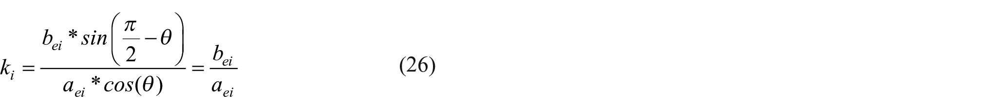
Then, we calculate the ratio between E_xx and G by dividing equation (11) by (16):

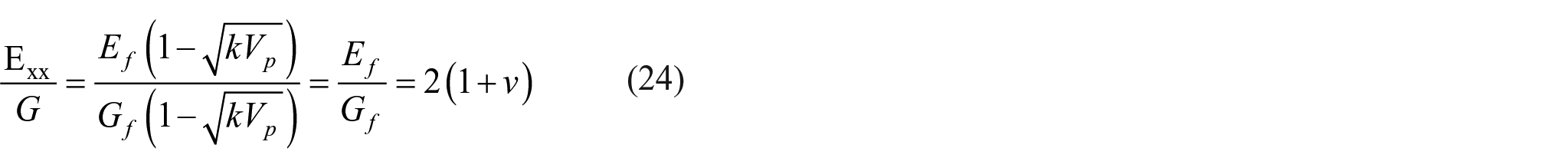
\frac{E_{xx}}{G} = \frac{E_{f} (1 - \sqrt{k V_{p}})}{G_{f} (1 - \sqrt{k V_{p}})} = \frac{E_{f}}{G_{f}}

(23)

Considering hypothesis 5, G_f=E_f ⁄ (2(1+v′)) is substituted into equation (23), giving

\frac{E_{xx}}{G} = \frac{E_{f} (1 - \sqrt{k V_{p}})}{G_{f} (1 - \sqrt{k V_{p}})} = \frac{E_{f}}{G_{f}} = 2 (1 + v)

(24)

Finally, substituting equations (17) and (24) into (2), the flexibility matrix is written in terms of the porosity and aspect ratios.

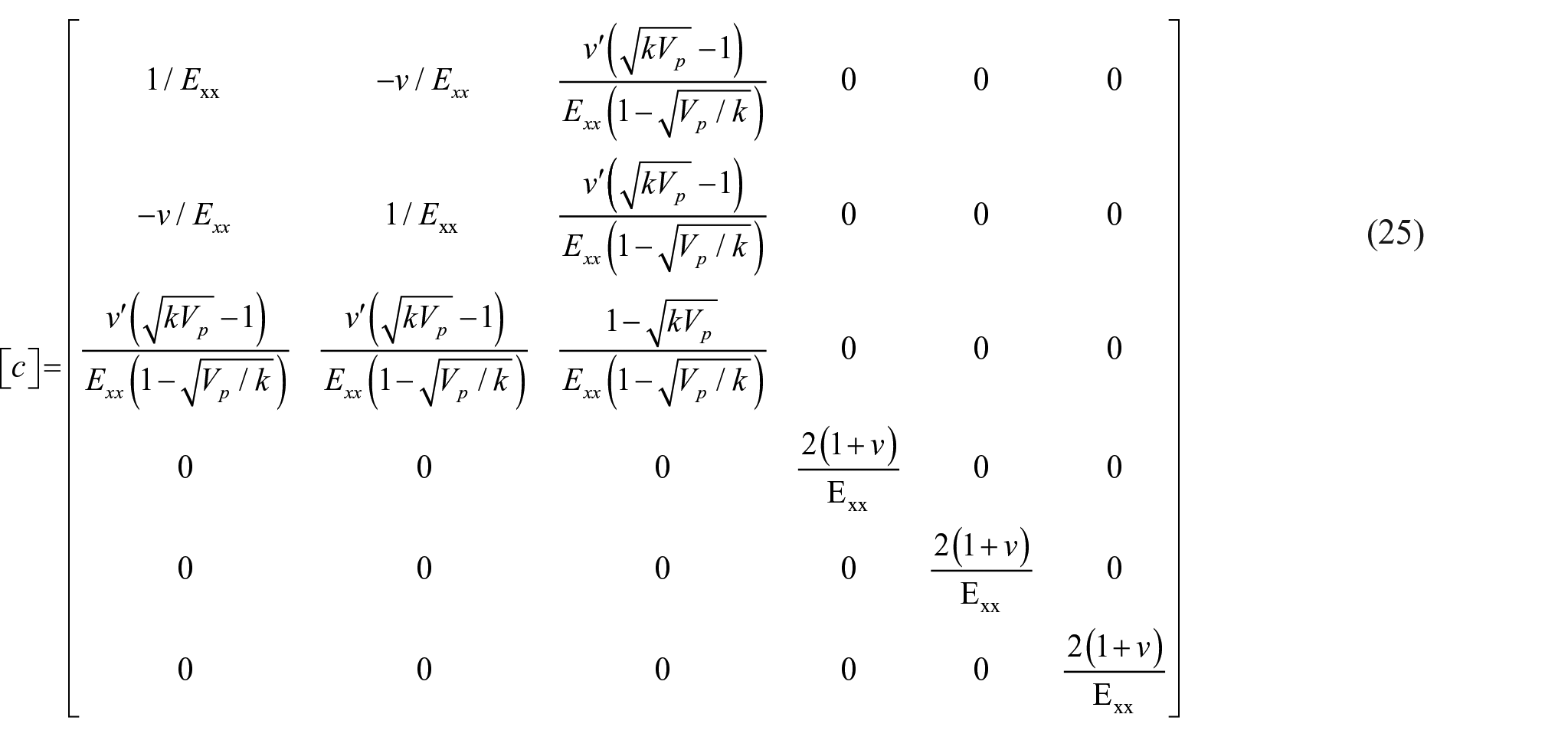
[c] = [\begin{matrix} 1 / E_{xx} & - v / E_{x x} & \frac{v^{'} (\sqrt{k V_{p}} - 1)}{E_{x x} (1 - \sqrt{V_{p} / k})} & 0 & 0 & 0 \\ - v / E_{x x} & 1 / E_{xx} & \frac{v^{'} (\sqrt{k V_{p}} - 1)}{E_{x x} (1 - \sqrt{V_{p} / k})} & 0 & 0 & 0 \\ \frac{v^{'} (\sqrt{k V_{p}} - 1)}{E_{x x} (1 - \sqrt{V_{p} / k})} & \frac{v^{'} (\sqrt{k V_{p}} - 1)}{E_{x x} (1 - \sqrt{V_{p} / k})} & \frac{1 - \sqrt{k V_{p}}}{E_{x x} (1 - \sqrt{V_{p} / k})} & 0 & 0 & 0 \\ 0 & 0 & 0 & \frac{2 (1 + v)}{E_{xx}} & 0 & 0 \\ 0 & 0 & 0 & 0 & \frac{2 (1 + v)}{E_{xx}} & 0 \\ 0 & 0 & 0 & 0 & 0 & \frac{2 (1 + v)}{E_{xx}} \end{matrix}]

(25)

Because the aspect ratio and porosity are usually constant for the same production process and raw material, they do not need to be measured every time. Only the E of the most accessible direction is required to predict the entire constitutive model. Here, in equation (25), the independent parameters that need to be identified are E_xx, v, v′, k, and V_p. Next, the experimental design used to identify these independent parameters is discussed. The model can calculate E_zz, which can help verify the model result by comparison with experiments.

Experimental design

Compression, FSEM, and porosity tests used to characterize the MPM are discussed. The compression tests were used to obtain the stress and strain data in all directions of the MPM, which are used to calculate the elastic moduli. In addition, the images collected during the compression test were used to identify Poisson’s ratio. The FSEM images were used to quantify the morphological features of the pores and porosity tests were used to quantify the MPM porosity.

Recycled corrugated cardboard was used to prepare MPM specimens. Mold No. 499 from Wuhan Peng Huan Packaging Co., Ltd. was selected for MPM sample preparation because it produces a flat area that satisfies the test requirements, as shown in Figure 5. This product was designed as an inner package for mechanical products with a large density. Specimens were collected from two regions of this mold: area (1) for strip compression tests and area (2) for compression tests normal to surface because the compression test normal to surface require 100 mm × 100 mm specimen size.²⁸

Figure 5.

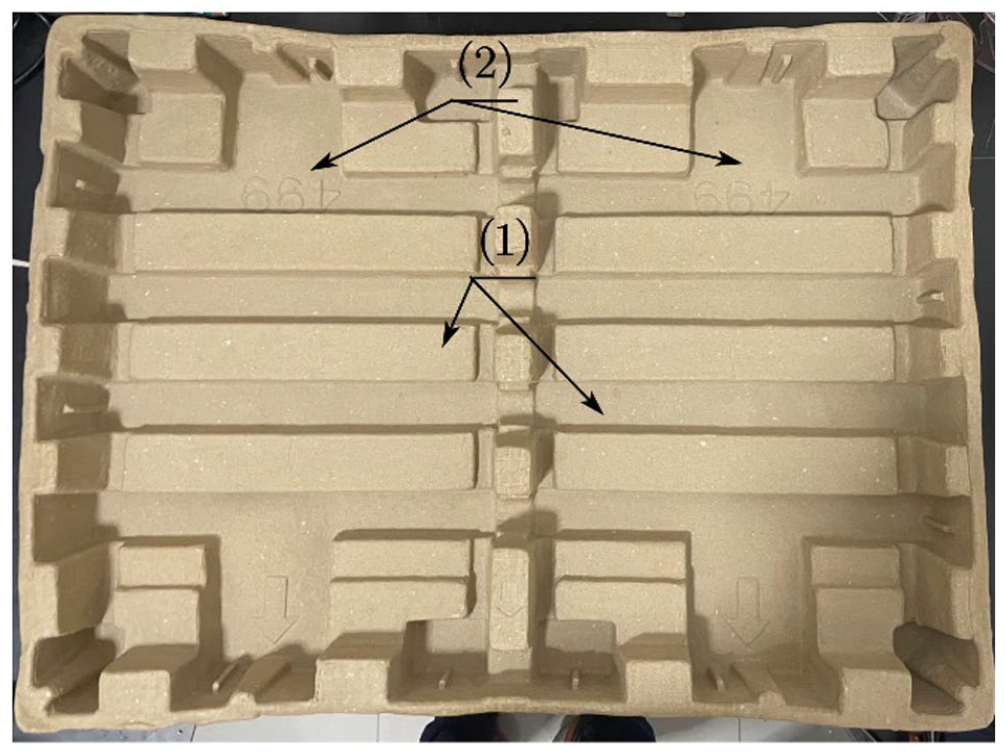
MPP sample used for testing. Area (1) was used for the compression tests in the surface plane, and area (2) for the compression tests normal to surface plane.

Poisson’s ratio based on digital image correlation

The digital image correlation method identifies the strain of different axes to calculate Poisson’s ratio (Figure 6). The first image (Figure 6(a)) is usually set as the reference image. Figure 6(b) shows the image with load applied, and (c) shows the superposition of the reference and test images. In this method, characteristic regions that appear in both the test and reference images (black dots in Figure 6) are aligned. In this way, the displacement of the reference point in the x and y directions (Δx and Δy, respectively) is calculated (Figure 6(c)). The displacement ratio of the horizontal and vertical axes is Poisson’s ratio. Therefore, v and v′ were identified in this way under different loads.

Figure 6.

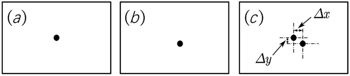
Schematic of the digital image correlation method: (a) original reference image, (b) test image under load, and (c) superposition of (a) and (b).

Some experimental factors that affect the results should be noted. (i) The camera needs to be placed as close as possible to the test sample, and the test area needs to fill the image. The number of pixels in the region of interest affects the test accuracy. (ii) The camera should be horizontally aligned with the ground, and the camera lens centerline should be perpendicular to the test sample surface during testing, as tilts introduce errors in the displacements in both directions. (iii) The ambient light level should be constant during a single test to ensure the accurate recognition of image features. In this study, the Ncorr program^29,30 in MatLAB was used for these calculations. Because this method requires images of the material in the original state and under load conditions, images were collected during compression tests.

Surface-plane compression test setup

The compression tests of the surface plane were used to identify E_xx and v. According to the TAPPI standard,³¹ the fixtures were designed to keep the exact distance between each test (Figure 7). The clamp assembly has four parts, which clamp both sides of the specimen, as shown in Figure 7. Screws connect the cover plate and base plate. The test samples were 15 mm wide and 60 mm long. An inward compressive force was applied to the sample at a velocity of 0.1 mm/min.

Figure 7.

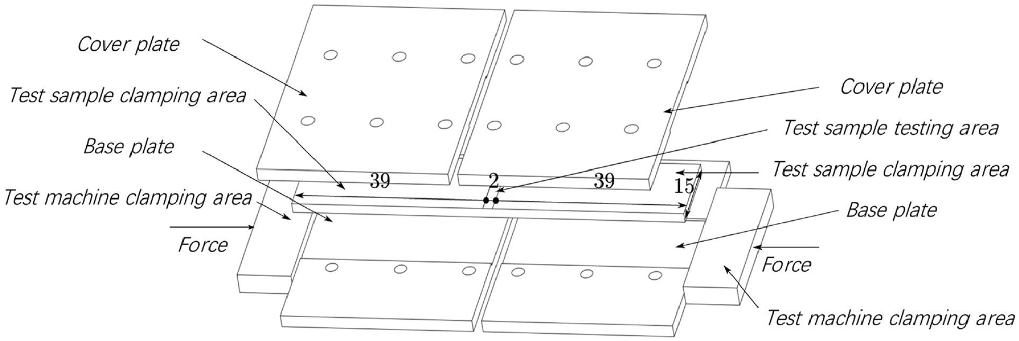
Schematic of the surface plane compressive test assembly and test sample geometry.

The compressive tests of the surface plane were performed using a SANSI CMT4104 universal tester. A Sony α7 camera with a Pentax 50 mm MARCO lens and a ring flash installed in front of the lens were used for image collection. White cardboard was placed behind the universal tester to provide a constant background color. The test was set as shown in Figure 8(a), and the actual test assembly is shown in Figure 8(b). The upper jig connects the force sensor and specimen clamp assembly. The lower jig connects the specimen clamp assembly and movable platform, which moves vertically to measure the displacement.

Figure 8.

(a) Surface plane compressive test setup: (1) Force sensor; (2) Upper jig; (3) Specimen clamp assembly; (4) Camera; (5) Lower jig; (6) Movable platform and (b) specimen clamp assembly: (1) Clamp plate; (2) Test specimen.

FSEM experiments

The pore ratio k was identified by FSEM (JSM-7600F, Japan Electronic Corporation). The samples were frozen in liquid nitrogen for 30 min and then broken with frozen forceps. A smooth cross-section was chosen, which was coated by gold spraying for 300 s. Due to the brittle manual fracture at low temperatures, several defects were present in the cross-section, and a piece with a completely flat area was selected for observation. Figure 9(a) shows a sample after low-temperature brittle fracture, Figure 9(b) shows the gold sprayer, and Figure 9(c) shows the samples mounted on the FSEM sample holder. The direction perpendicular to the surface plane was mainly observed, along with the surface plane.

Figure 9.

Sample preparation for FSEM: (a) sample after low-temperature brittle fracture, (b) gold spraying system, and (c) FSEM sample holder loaded with samples.

The FSEM images need a morphological opening operation to remove isolated pixel. The local uniform brightness method was used to convert the image to a binary image. After noise reduction of the binary image, the edge coordinates of each pore in the picture were extracted according to pore-size sorting. Then, after extraction each single pore image and clean noise, ellipse fitting was performed to simulate each pore as an ellipse. Finally, the average ratio k for all ellipses in the image was obtained from the weighted average of each ellipse. After removing the noise, the image was analyzed. The pores in the image were identified and fit ellipses.

Porosity measurements

The porosity V_p of the material was measured using porosity tests with a BSD-TD-K automatic true density and porosity analyzer (Beishide Instrument Technology Co., Ltd., China). After precompression, the sample was cut into a size of 25 mm × 50 mm, according to standard GB/T 10799-2008.³² After drying and standing at room temperature for 72 h, multiple slices were layered until the thickness reached ~25 mm, shows in Figure 10 (a). And then sample holder being loaded into the equipment, shows in Figure 10 (b). The schematic diagram of the test setup in Figure 10 (c) can help understanding this test, which uses the gas replacement method to determine the skeleton volume of the sample chamber. Helium is used to clean the gas circuit under negative pressure after putting the test samples into the sample chamber and loading them into the instrument. Then, a certain amount of helium is loaded into the baseline chamber under a certain pressure, following with the test valve is opened to read the pressure in the presence of the sample. The pressure difference between the test valve close and open is used to calculate the helium volume expansion, which is equivalent to the total pore volume. Then, the porosity can be calculated by the volume of specimen divided by the helium volume expansion.

Figure 10.

Porosity measurements by the gas expansion replacement method: (a) sample chamber filled with molded pulp specimens, (b) sample holder being loaded into the equipment, and (c) schematic diagram of the test setup.

Compressive tests normal to surface plane

v′ the parameter of model and E′_zz values for verification of the model were obtained by compressive tests. This test requires sensor range larger than 20kN, so a Shimadzu AG-IC 100 kN high-temperature endurance testing machine was used. The samples were prepared following a GB standard,²⁸ with dimensions of 100 mm×100 mm, where the thickness of a single piece was <25 mm. The test was performed by stacking multiple pieces and the test was set as shown in Figure 11. The camera settings were identical to those used in the previously discussed measurements. The pressure plate is smaller than 100 mm×100 mm, so two thick steel plates were installed on both sides of the plates. First, the initial specimen thickness was measured, and then the specimen was pre-compressed to 20% strain 10 times (over approximately 30 min). Then, the pre-compressed thickness was measured, and this thickness was used as the starting thickness for the compressive tests. Finally, the compressive tests were performed from the pre-compressed thickness with a 12 mm/min velocity. The test was stopped when the stress increased rapidly which indicates the material failure of the test.

Figure 11.

Compressive test normal to surface plane setup. (1) Force sensor; (2) Upper-pressure plate; (3) Test specimen; (4) Lower-pressure plate; (5) Camera.

Parameter identification and verification

The data collected using the methods described previously are discussed here. The least squares method was used to fit the elastic moduli curves in the elastic region. The Ncorr program^29,30 and the MatLAB image toolbox were used for digital image correlation and identifying the Poisson’s ratios.

Surface plane compressive test results

The dimensions of the specimens used in the compressive tests after incubation for 24 h at 26°C. The compressive stress–strain curves in Figure 12 show a similar relationship for all samples for strains below 0.03. The maximum stress values indicate the fiber connection failure are also similar, except for sample 4. At the end of compression, the stress falls to 1.8 MPa indicate the failure fiber accumulation, for all samples except sample 2, which has a much larger plateau value. The stress data below a strain of 0.015 (linear stress–strain relationship) is defined as the elastic stage. A linear fit was applied to the data in this region and the average value of the slope was calculated to obtained E_xx = 123.15 MPa.

Figure 12.

Surface plane compression test result and elastic stage linear fit.

The images from digital image correlation with the Ncorr method^29,30 are shown as the horizontal and vertical displacements. These data were used to calculate the strain in these two directions. The results for sample 3 are shown in Figure 14, as a representative sample. Figure 13(a) and (b) are the calculated displacement data, and (c, d) are the calculated strain data. By calculating the overall strain of the test area, the Poisson’s ratio at a specific time can be obtained by calculating the ratio between the vertical and horizental strain. Over the entire experimental process, the fluctuations in the Poisson’s ratio data can be eliminated by linear fitting, as shown in Figure 14, which gave a result of v = 0.8678.

Figure 13.

Digital image correlation results from the compressive tests of the surface plane. Displacement results in the (a) horizontal and (b) vertical directions. Strain results in the (c) horizontal and (d) vertical directions.

Figure 14.

Poisson’s ratio test data (and its linear fit) from compression testing of the surface plane.

FSEM results

An original FSEM image is shown in Figure 15(a), while the corresponding binarized image is shown in Figure 15(b), with some noise points. The largest pore in Figure 15(a) fit as an ellipse is shown in Figure 16(a). The long–short axis ratio of the ith ellipse (k_i) was calculated as follows:

k_{i} = \frac{b_{e i} * s i n (\frac{π}{2} - θ)}{a_{e i} * c o s (θ)} = \frac{b_{e i}}{a_{e i}}

(26)

Figure 15.

Treatment of FSEM images to obtain pore information: (a) original image and (b) binarized image.

Figure 16.

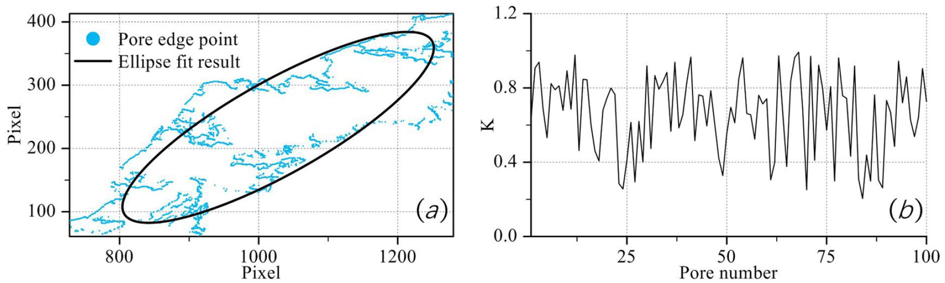
(a) Pore edge points and ellipse fitting results of samples observed normal to surface plane and (b) axial ratio of the ellipse of the 100 largest pores.

Here, i is the number of the pore sorted by pore size from largest to smallest.

Figure 16(b) shows the k values for the 100 largest pores. The overall k values was calculated by weighted averaging, as follows:

k = \frac{\sum_{i = 1}^{n} k_{i} * a_{i}}{\sum_{i = 1}^{n} a_{i}}

(27)

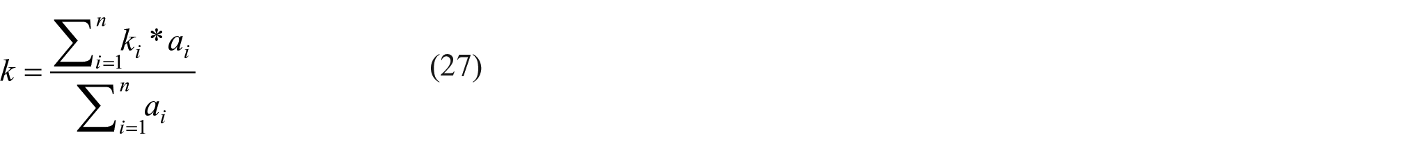
Here, a_i is the size of the ith pore, n is the number of pores. The average k was determined to be 0.7034.

Porosity results

The porosity test results are processed by material density and weight to correct the error of the measured test sample volume of MPM. Six porosity measurements were performed for each group of samples, and the results shows in Figure 17 were averaged to give V_p = 69.79 ± 0.11%. The porosity variation at ~0.158%, different test cycles of the same sample group variation within ~0.10%, indicates that different samples of the MPM remains stable.

Figure 17.

Porosity test result of MPM.

Compressive tests normal to surface plane

The compression test normal to surface plane image results are used for identify the v′ value.Figure 18(a) and (b) are the calculated displacement data, and (c, d) are the calculated strain data. By calculating the overall strain of the test area, the Poisson’s ratio at a specific time can be obtained by calculating the ratio between the vertical and horizontal strain. Over the entire experimental process, the fluctuations in the Poisson’s ratio data can be eliminated by linear fitting, as shown in Figure 19, a v′ value of 0.014 was determined.

Figure 18.

Digital image correlation results from the compressive tests normal to surface plane. Displacement results in the (a) horizontal and (b) vertical directions. Strain results in the (c) horizontal and (d) vertical directions.

Figure 19.

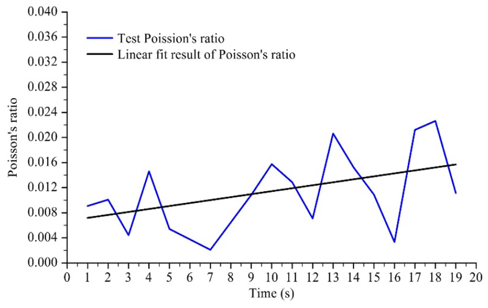
Poisson’s ratio and its linear fit measured during compression normal to surface plane.

Parameter summary and model verification

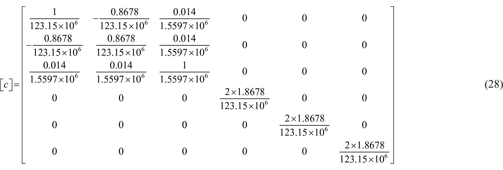
The results obtained from the analysis of the above results are: elastic modulus E_xx = 123.15 MPa, v = 0.8678, v′ = 0.014, k = 0.7034, and V_p = 0.6979. The E_zz was calculated using equation (17) as 1.5597 MPa. In addition, using equation (26), we calculated G = 32.967 MPa. The parameters of the flexibility matrix were obtained as follows:

[c] = [\begin{matrix} \frac{1}{123.15 \times 10^{6}} & - \frac{0.8678}{123.15 \times 10^{6}} & \frac{0.014}{1.5597 \times 10^{6}} & 0 & 0 & 0 \\ - \frac{0.8678}{123.15 \times 10^{6}} & \frac{0.8678}{123.15 \times 10^{6}} & \frac{0.014}{1.5597 \times 10^{6}} & 0 & 0 & 0 \\ \frac{0.014}{1.5597 \times 10^{6}} & \frac{0.014}{1.5597 \times 10^{6}} & \frac{1}{1.5597 \times 10^{6}} & 0 & 0 & 0 \\ 0 & 0 & 0 & \frac{2 \times 1.8678}{123.15 \times 10^{6}} & 0 & 0 \\ 0 & 0 & 0 & 0 & \frac{2 \times 1.8678}{123.15 \times 10^{6}} & 0 \\ 0 & 0 & 0 & 0 & 0 & \frac{2 \times 1.8678}{123.15 \times 10^{6}} \end{matrix}]

(28)

The experimental stress–strain curves measured normal to surface plane direction are shown in Figure 20. The first half of the curve was modeled with a linear fit, giving E′_zz = 1.5368 MPa. These curves indicate that the MPM is an elastoplastic material.

Figure 20.

The compression test normal to surface plane result and elastic stage linear fit.

According to equation (17), it can be inferred that E_zz can be determined by E_xx, V_p, and k. By comparing the calculated value of E_zz with the experimental result, it can be observed that the accuracy of the calculated value is heavily influenced by the error range of E_xx, whereas the error range of V_p has a minor effect. The actual error range is smaller than the experimental range of E′_zz. The mean value, upper and lower deviation, as well as the deviation percentage, are presented in Table 1.

Table 1.

Values and errors for E_zz calculation.

Parameter	Mean value	Upper deviation	Upper deviation percentage	Lower deviation	Lower deviation percentage
E _xx	123.15 MPa	7.7127 MPa	6.26%	–6.7526 MPa	–5.48%
V_p	69.79%	0.11%	16%	–0.11%	16%
E _zz	1.5998 MPa	0.1002 MPa	6.26%	–0.0877 MPa	–5.48%
E′_zz	1.5368 MPa	0.2546 MPa	16.56%	–0.2052 MPa	–13.35%

Conclusions

The aim of this study was to identify the basic constitutive parameters of molded pulp made from recycled paperboard using digital microscopy, compressive tests, and porosity measurements. This study used FSEM to observe the fiber distribution in an MPM, and the morphological information was used to build a transversely isotropic constitutive model based on meso-structural mechanics, which was verified by a comparison with compressive stress–strain data measured normal to surface plane direction. The elastic modulus values measured along different axes were significantly different; the values along the surface-plane are ~80 times higher than that along the normal to surface plane direction. This is attributed to the fibers in the surface-plane being randomly bonded with other fibers, while stratification was observed along the normal to surface plane. This also resulted in Poisson’s ratios that varied by a factor of ~62 between the different directions.

Because the stress–strain curves of the surface plane and normal to the surface plane compression are different in the elastic–plastic stage, the proposed method cannot be used to predict the stress–strain curves for such a model. However, in the case of an elastic modulus, the calculated and experimental mean results varied by 4.7%. The normal to surface direction test results exhibit a deviation range of -13.5% to +16.5%, whereas the deviation range of the results obtained through modeling calculation is only −5.48% to 6.26%, indicating greater precision. Some possible sources of experimental uncertainty include the following:

1. Electron drift during FSEM imaging, resulting in distortion of the images.

2. Errors introduced by the binarization, noise removal, and ellipse-fitting steps during image analysis that distort the real pore edges.

3. Errors during porosity tests arising from the incomplete filling of the gas into the sample (i.e. overestimating the porosity).

The test results are considered acceptable because an isotropic material is usually assumed in materials simulations. However, the simulation accuracy can be improved by assuming a transverse isotropic material.

In future work, the method for determining the pore morphology could be enhanced to increase the reliability of the pore ratio data. In addition, the viscoelastic part of the compressive tests for the Oxy plane and Oz axis needs to be modeled. The constitutive model built here could be improved by combining it with the viscoelastic models of the two axes to support the simulation of MPP design.

Footnotes

Declaration of conflicting interests

The author(s) declared no potential conflicts of interest with respect to the research, authorship, and/or publication of this article.

Funding

The author(s) received no financial support for the research, authorship, and/or publication of this article.

ORCID iD

Zhihang Li

References

European Union. Sustainable waste management in a circular economy. A Policy Brief from the Policy Learning Platform on Environment and resource efficiency, https://www.switch-asia.eu/site/assets/files/2597/policy_brief_on_waste_management.pdf (2020, accessed 24 July 2022).

Ogunmakinde

OE.

A review of Circular Economy Development Models in China, Germany and Japan. Recycl 2019; 4: 27.

Hoffmann

Compression and cushioning characteristics of moulded pulp packaging. Packag Technol Sci 2000; 13: 211–220.

Wang

Guo

Luo

GL.

Mechanical Properties of molded pulp pallet. Appl Mech Mater 2012; 121-126: 216–220.

Wang

Cai

Jing

Molded pulp material structure parameters on the performance of the Buffer. Energy Proc 2012; 17: 1872–1877.

Tanninen

Leminen

Matthews

, et al. Measurement of changes in torsional stiffness of press-formed paperboard packages induced by heat load utilizing a developed measuring device. Packag Technol Sci 2021; 34: 641–650.

Gurav

Bereznitski

Heidweiller

, et al. Mechanical properties of paper-pulp packaging. Compos Sci Technol 2003; 63: 1325–1334.

Ping

, et al. Investigation of the mechanical properties of molded pulp with DICM. Packag Eng 2004; 25: 168–170.

Shao

Wang

, et al. Mechanical properties of molded pulp under various loading conditions. Packag Eng 2007; 28: 10–13.

10.

Zhang

Research on Cushion Performance and Reliability about Paper-pulp Packaging Structure. PhD Thesis, Wuhan University of Technology, 2007.

11.

Wang

Guo

Modification of constitutive equation fitting of moulded pulp material. Packag Eng 2009; 30: 11–13.

12.

Wang

Miao

, et al. Research on compression mechanical behaviors and constitutive relation of moulded pulp material. J Mech Strength 2009; 31: 382–386.

13.

Wang

Chen

Mechanical behaviors of molded pulp material. In: ICEM 2008: International Conference on Experimental Mechanics 2008, SPIE, pp.1448–1452.

14.

Wang

HW.

Short span compressive stress-strain relation and model of molded pulp material. Key Eng Mater 2011; 450: 202–205.

15.

Wang

Numerical Analysis of elastoplasticity for large-scaled moulded pulp pallet. Packag J 2011; 3: 7–10.

16.

Yang

Berthold

Berglund

LA.

Preserving cellulose structure: delignified wood fibers for paper structures of high strength and transparency. Biomacromolecules 2018; 19: 3020–3029.

17.

Yang

Berglund

LA.

Recycling without fiber Degradation—Strong paper structures for 3D forming based on nanostructurally tailored wood holocellulose fibers. ACS Sustain Chem Eng 2020; 8: 1146–1154.

18.

Rattanawongkun

Kerddonfag

Tawichai

, et al. Improving agricultural waste pulps via self-blending concept with potential use in moulded pulp packaging. J Environ Chem Eng 2020; 8: 104320.

19.

Rattanawongkun

Kunfong

Klayya

, et al. Comparison of molded pulps from rice straw, pineapple leaf and banana stem pulps. ScienceAsia 2020; 46S: 79.

20.

Simon

J-W.

A review of recent trends and challenges in computational modeling of paper and paperboard at different scales. Arch Comput Methods Eng 2021; 28: 2409–2428.

21.

Alava

Niskanen

The physics of paper. Rep Prog Phys 2006; 69: 669–723.

22.

Potashev

Gur’ev

Filippov

, et al. Structure deformation features of molded pulp products. Lesn Zhurnal For J 2019; 2: 119–129.

23.

Hua

Yang

Fei

, et al. Poisson’s ratios of molded pulp materials by digital image correlation method and uniaxial tensile test. J Eng Fibers Fabr 2020; 15: 1–10.

24.

Alzweighi

Mansour

Lahti

, et al. The influence of structural variations on the constitutive response and strain variations in thin fibrous materials. Acta Mater 2021; 203: 116460.

25.

Gibson

RF.

Principles of Composite Material Mechanics. 4th ed. Boca Raton, FL: CRC Press, 2016.

26.

Panshin

AJ.

Textbook of wood technology: structure, identification, properties, and uses of the commercial woods of the United States and Canada. 4th ed. New York, NY: McGraw-Hill, 1980.

27.

Debnath

Sarder

Pal

, et al. Molded pulp products for sustainable packaging: Production Rate Challenges and product opportunities. Bioresour 2022; 17: 3810–3870.

28.

GB/T 8168:2008. Testing method of static compression for packaging cushioning materials. Standardization Administration of China, 2008.

29.

Blaber

Adair

Antoniou

Ncorr: open-source 2D digital image correlation Matlab software. Exp Mech 2015; 55: 1105–1122.

30.

Kumar

Aravind

Hossiney

Digital image correlation (DIC) for measuring strain in brick masonry specimen using Ncorr open source 2D MATLAB program. Results Eng 2019; 4: 100061.

31.

TAPPI T826:2013. Short span compressive strength of containerboard. Technical Association of the Pulp and Paper Industry, 2013.

32.

GB/T 10799:2008. Rigid cellular plastics-determination of the volume percentage of open cells and of closed cells. Standardization Administration of China, 2008.

Constitutive model and experimental study of molded pulp material

Abstract

Keywords

Introduction

Constitutive model of molded pulp materials

Fiber distribution of molded pulp

Correlation between independent variables of the constitutive model based on meso-structural mechanics

Experimental design

Poisson’s ratio based on digital image correlation

Surface-plane compression test setup

FSEM experiments

Porosity measurements

Compressive tests normal to surface plane

Parameter identification and verification

Surface plane compressive test results

FSEM results

Porosity results

Compressive tests normal to surface plane

Parameter summary and model verification

Conclusions

Footnotes

Declaration of conflicting interests

Funding

ORCID iD

References