Sage Journals: Discover world-class research

Abstract

Fabric defect detection is an important quality inspection process in the textile industry. A fabric defect detection system based on transfer learning and an improved Faster R-CNN is proposed to solve the problems of low detection accuracy, general convergence ability, and poor detection effect for small target defects in existing fabric defect detection algorithms. The pre-trained weights on the big dataset Imagenet are first extracted for transfer learning. Images are then input into the improved Faster R-CNN network, while the ResNet50 and ROI Align are used to replace the original VGG16 feature extraction network structure and a region of interest (ROI) pooling layer to avoid the problems of region mismatch caused by two quantizations from ROI pooling. The region proposal network (RPN) is combined with the multi-scale feature pyramid FPN to generate candidate regions with richer semantic information and project them onto the feature map to obtain the corresponding feature matrix. Cascaded modules are integrated and different IoU thresholds are used for each level to distinguish positive and negative samples. Finally, the softmax classifier is adopted to identify the image and obtain the predictions. The experimental results show that the detection accuracy and convergence ability of the improved Faster R-CNN are greatly enhanced compared with the current mainstream models, which provides a reference for future fabric defect detection methods.

Keywords

Transfer learning fabric defect detection Faster R-CNN Cascade

Introduction

In the textile industry, various objective factors such as machine failure and yarn fracture readily cause fabric defects, which affects the fabric quality and causes significant economic losses to enterprises. Automatic defect detection plays a key role in controlling product quality.¹ For some time, the detection process of fabric defects is performed by manual visual inspection. The high costs of manual cloth inspection have affected the detection rate,² and even the most skilled cloth inspection workers can only find approximately 70% of defects.³ Further, long-term inspection damages human vision. While some testing equipment has been successfully applied in textile processing, such as EVS I-Tex2000, Barco Visions Cyclops, and MQT, limitations of intellectual property rights have prevented the details of these fabric defect detection algorithms from going public, and existing equipment lacks adaptive abilities for a variety of fabric images.⁴ Therefore, automatic detection of fabric defects is needed to reduce waste in both time and costs from manual detection⁵ to improve the overall quality of products and strengthen the competitiveness of textile exports. The directional characteristics of fabric defects can be divided into three categories: (1) weft defects; (2) longitudinal defects; and (3) defects without directional features. The purpose of automatic detection is to determine the position and type of defect in fabrics without any human inference. Automatic fabric defect detection can overcome the shortcomings of manual detection, reduce detection costs, and maintain a high success rate (90%).⁶

Traditional fabric defect detection methods are roughly divided into four categories: statistical,⁷ spectral analysis,⁸ model-based,⁹ and low-rank decomposition.¹⁰ Ji et al.¹¹ proposed a detection method based on weighted low rank decomposition and Laplacian regularization term. By introducing Laplacian regularization term to expand the distance between background and defect area, the robustness of the model is enhanced. Yapi et al.¹² proposed using supervised learning to classify defective and flawless fabrics. Basu et al.¹³ studied fabric defect detection through a support vector machine (SVM) and other classifiers. Han and Xu¹⁴ developed a template matching method from the statistical data of fabric textures and combined it with threshold method to detect small defects. Abdellah et al.¹⁵ used morphological technology and geometric data to detect small defects on fabric surfaces, applied Sobel edge detection and morphological processing to identify defects, and determined the type of defect by measuring the domain, environment, and density of the obtained image. Model-based detection methods use a random process to represent fabric textures. That is, the texture image is regarded as the sample generated by random processes in the image space. Defect detection is regarded as a hypothesis testing problem of statistical information derived from the model. The representative models are primarily the Gaussian-Markov random field (GMRF)¹⁶ and Gaussian mixture¹⁷ models. However, these methods lack universality, have difficulty detecting fabric images with complex textures, and have low detection accuracies for small defect targets.

The concept of deep learning has developed in recent years. As one of the main frameworks of deep learning is the convolutional neural network (CNN), which is widely used in image recognition,¹⁸ segmentation,¹⁹ object detection,²⁰ and 3D perception.^21,22 Convolutional neural network can directly process the original test image and generate multi-layer features of complex fabric texture image through multiple nonlinear transformations.²³ Compared with traditional target detection methods, those based on deep learning have stronger robustness and higher detection accuracies. The main purpose of object detection is to locate ROI in the image and determine their categories. Object detection algorithms based on deep learning can be divided into two-stage and one-stage approaches. Two-stage object detection algorithms include two stages of target detection: the generation of candidate box and recognition of target category. These include the R-CNN, SPP-Net, Fast R-CNN, Faster R-CNN, Mask RCNN, R-FCN, FPN, Cascade RCNN, etc; Representative models of one stage target detection algorithm include YOLO, SSD, Retina Net, RefineDet, etc. Recently, algorithms such as CornerNet, CenterNet, Cascade Faster RCNN have also appeared one after another. More complex and in-depth visual effects are used in these algorithms to extract features from images to generate image regions.

Since the 1980s, many scholars have committed to using deep learning technologies for fabric defect detection and have proposed various associated algorithms. Ming et al.²⁴ combined the GAN with the Faster R-CNN, where the former was utilized to expand the dataset and the latter was used for fabric defect detection. However, that process required significant time for detection and cannot meet industrial requirements. Based on the SSD algorithm, ChuanHua et al.²⁵ used an improved selective search approach to selectively examine the target area and complete detection from coarse to fine. However, this algorithm had difficulty detecting small target defects. Xu et al.²⁶ applied the path-enhanced feature pyramid network (PAFPN) and edge detection branch to the Mask RCNN algorithm, but the detection accuracy was relatively poor. Ngan et al.²⁷ proposed a wavelet gold image subtraction (WGIS) method based on wavelet preprocessing to improve the traditional image subtraction (TIS) to detect defects in patterned fabrics or repeated pattern textures. The overall success rate of this method for detecting 30 defective fabric images was 96.7%, but the versatility was poor. Inspired by the mechanism of human visual perception and memory, Zhao et al.²⁸ proposed an integrated CNN model based on the visual long-term and short-term memory (VLSTM), which effectively solved the problem when fabric defects are not obvious in texture backgrounds and several defect types become easily confused and are difficult to be distinguished. However, the accuracy of the results depends on the degree and size of defect variations; Zhao et al.²⁹ proposed a Cascade Faster RCNN network, which uses multi-layer Cascade detectors to pre classify fabric defects and the non maximum suppression algorithm is optimized, which significantly improves the fabric defect detection effect, Shenbao et al.³⁰ improved Cascade RCNN by adding online difficult case mining and variable convolution V2 to improve the detection accuracy, so as to better meet the needs of fabric defect detection. Jing and Ren use RGB cumulative average method (RGBAAM) and image pyramid to detect printed fabric defects. This method can effectively segment printed fabric defects with low calculation cost, but the detection speed is relatively slow.³¹ Liu et al.⁴ proposed a weakly supervised shallow network, which integrates Link-SE (L-SE) module and Dilation Up-Weight CAM (DUW-CAM), fabric background features are suppressed through DUW-CAM with attention mechanism, and defect areas are located more accurately, but the calculation process is cumbersome.

Currently, computer vision has made great achievements in some fields, but these successes require the support of significant amounts of data. In practical applications, there is often a lack of sufficient labeled samples, while test samples and training samples do not meet the same distribution assumptions.³² In particular, training deep neural networks requires hundreds of thousands or even millions of data points to achieve good results. In image classification, data are relatively precious, and usually only a relatively small number of images can be collected. Therefore, transfer learning can be used to solve the problem of insufficient available data.³³ Transfer learning is a method that uses a previously trained model for a separate problem as a starting point to solve related problems. Therefore, the data required for domain-specific tasks can be significantly reduced.^34–36 Starting from the existing network and training weights reduces the training cost and improves the training efficiency.

The four common implementation methods for transfer learning include (1) sample transfer, (2) feature transfer, (3) model transfer, and (4) relationship transfer.³⁷ Taking the residual network as an example, Junli and Kai³³ studied the application of transfer learning in fabric defect recognition and compared its effect on two datasets of different sizes. It was concluded that when the dataset was comparatively small, the recognition rate of the model could be improved using transfer learning. Xiaona et al.³⁴ proposed image change detection in panoramic blocks based on the Segnet network and transfer learning. The experimental results showed that their proposed method had a higher change detection accuracy than previous methods. Yosinski et al.³⁵ studied the portability of deep learning based on CNNs and used the AlexNet structure for transfer learning layer-by-layer with fine-tuning as a comparative study. They showed that the model-based transfer learning method is effective, and the anterior layers of deep learning can learn common features, which improved the effects of transfer learning on the anterior layers. Thus, the combination of transfer and deep learning can provide good model detection results when there are less available data.

Existing problems in fabric defect detection based on deep learning primarily include the following aspects. (1) There is a long training time using fabric images due to the deep network layer and complex structure from the first to the last convolution layers. (2) There are many small target defects in fabrics, which gives a poor detection effect and accuracy. The region proposal network (RPN) acts on the last layer of the CNN to detect large targets. Although this layer contains rich semantic information, it cannot extract small target information, which indicates it cannot effectively detect small target defects. The two quantization and integration operations of ROI Pooling greatly reduce the accuracy, and the feature size output is not sufficiently accurate. (3) There is a lack of fabric defect samples as most existing defect datasets are relatively small and lack defect diversity.

Therefore, aiming at the problems in current fabric defect detection algorithms, this paper takes the Faster R-CNN network in a deep CNN as the framework and proposes a fabric defect detection algorithm based on transfer learning and an improved Faster R-CNN. Improving the Faster R-CNN network allows performing transfer learning using pre-trained weights on the big dataset Imagenet (computer vision dataset that covers most image categories seen in life), while ResNet50 is used as the feature extraction network. The ROI Align is selected to replace the ROI pooling, and the FPN multi-scale feature pyramid is integrated to realize fabric defect detection.

Faster R-CNN algorithm based on transfer learning and its improvement

Framework of original Faster R-CNN network and its disadvantages

In 2012, Hinton and Krizhevsky proposed the AlexNet CNN, which laid a solid foundation for a series of future improved CNNs^36,38 followed by target recognition algorithms such as the Faster R-CNN, YOLO,³⁹ and SSD.⁴⁰ The Faster R-CNN algorithm has experienced a development process from the RCNN⁴¹ to the Fast R-CNN⁴² and then to the Faster R-CNN. The Faster R-CNN algorithm process is as follows. (1) Input an image into the CNN to obtain the feature map. (2) Input the convolutional feature to the RPN to obtain the candidate box feature information. (3) Use classifiers to determine whether the extracted features from the candidate box belong to a specific class. (4) Use regression for a feature candidate box to further adjust its position.

The RPN is added to the current Faster R-CNN structure, which improves the detection accuracy, versatility, and robustness. However, fabric defect detection has the following shortcomings. (1) The VGG16 is used as the feature extraction network, which has a deep structure that leads to long training times, difficult parameter adjustments, and large storage capacities while tending to face gradient disappearance or explosion. When the network is stacked to a certain depth, the results of the deep network are worse than that of shallow networks. (2) As the CNN goes from shallow to deep, semantic features become richer, but the feature map becomes smaller, which reduces the resolution. The size distribution of fabric defects is uneven; thus, the original algorithm recognition and positioning accuracy are not sufficiently accurate. (3) There are two quantization processes in the ROI pooling process of the original Faster R-CNN network. This results in deviations in the obtained candidate box relative to the initial position, which affects the accuracy of fabric defect detection. (4) There are many categories of defect samples, including many unusual categories that result in the lack of dataset samples.

Improved Faster R-CNN network framework based on transfer learning

Aiming at the shortcomings of the original Faster R-CNN and the lack of samples and datasets, this paper made the following improvements:

(1) Use the ResNet50 instead of the VGG16 network for feature extraction in the improved Faster R-CNN. This reduces both the complexity of the improved algorithm and the number of required parameters. The network depth is deeper, and the problem of gradient vanishing does not occur while ensuring the accuracy of fabric defect classification. This solves the gradient degradation problem of deep networks.

(2) Add an FPN to the original Faster R-CNN network. The shallow and high-level features are connected, and the FPN and RPN are fused to accurately locate and detect defects for small target fabrics in the dataset.

(3) Replace ROI pooling with ROI Align. This cancels quantization and avoids ignoring some details when selecting defects to accurately locate the candidate box.

(4) Introduce transfer learning to further reduce training time. The effect of transfer learning is largely impacted by the similarity between the new dataset and the source dataset. The Imagenet dataset contains 1000 common image categories of nature with some characteristics being universal to a certain extent thus, the ResNet50 model pre-trained weights from the large Imagenet dataset is selected to initialize the weights of the improved algorithm. Then, the fabric defect dataset is used to retrain the top-level convolution network, which updates the parameters by fine-tuning so that the training time is greatly reduced without affecting the model accuracy. The ideal results are then quickly trained. The improved Cascade Faster R-CNN network structure is shown in Figure 1.

Figure 1.

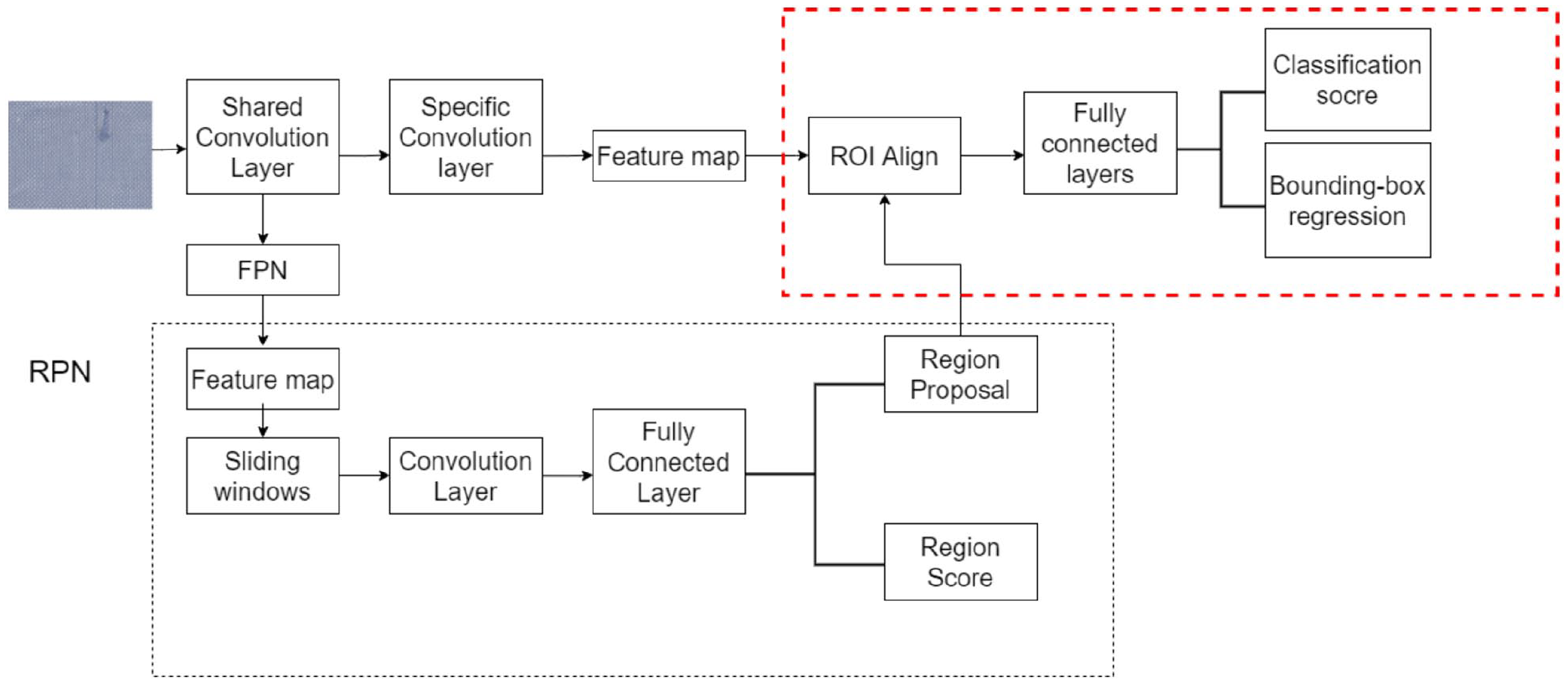
Improved Cascade Faster R-CNN network structure diagram.

The research steps of the improved Faster R-CNN algorithm are as follows. The image is input into the feature extraction network of ResNet50 and FPN, and the obtained feature map is input into the RPN to acquire approximately 2000 target suggestion frames. The feature matrix is obtained based on the corresponding relationship between the original image and the feature map. The feature matrix corresponding to each proposal is input into the ROI Align layer. The feature map of size 7 × 7 is flattened using two fully connected layers, and the prediction layer is regressed from the category prediction layer and the boundary frame. Finally, a series of processing steps is performed to accurately predict target defects.

Selection of ResNet network structure

The residual net (ResNet) is used as the feature extraction network, which was proposed by He et al.⁴³ Its core idea is to use a residual learning structure that regards the superimposed network layer as an identity map to avoid the common “degradation phenomenon” in deep network training. The standard residual structure is as shown in Figure 2.

Figure 2.

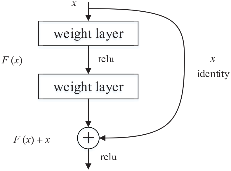
Standard residual structure diagram.

The residual unit can be expressed as:

y_{l} = F (x_{l}) + x_{l}

(1)

x_{l + 1} = f (y_{l})

(2)

where $x_{l}$ and $x_{l + 1}$ represent the input and output of the L-th residual unit, respectively, $f$ is the residual function that represents the learned residual, and $F$ is the relu activation function. Therefore, the learning characteristics from a shallow to deep L are:

x_{L} = x_{l} + \sum_{i = l}^{L - 1} F (x_{i}, W_{i})

(3)

Using the chain rule, the gradient of the reverse process can be obtained as:

\frac{\partial l o s s}{\partial_{x_{l}}} = \frac{\partial l o s s}{\partial_{x_{L}}} . \frac{\partial_{x_{L}}}{\partial_{x_{l}}} = \frac{\partial l o s s}{\partial_{x_{L}}} . (1 + \frac{\partial}{\partial_{x_{L}}} \sum_{i = l}^{L - 1} F (x_{i}, W_{i}))

(4)

The ResNet network can be divided into ResNet18, ResNet34, ResNet50, ResNet101, and ResNet152 based on the number of layers. As the shallow ResNet18 and ResNet34 networks have low detection accuracies and the deep ResNet101 and ResNet152 networks have long detection times, the ResNet residual structure with a moderate depth is selected here, which is composed of multiple convolutional groups. The structure of ResNet50 network is shown in Table 1.

Table 1.

Structure of the ResNet50 network.

Convolution layer name	ResNet50
Conv1	7 × 7, 64, stride2, 3 × 3 max pool, stride2
Conv2_x	$[\begin{matrix} 1 \times 1, 64 \\ 3 \times 3, 64 \\ 1 \times 1, 256 \end{matrix}] \times 3$
Conv3_x	$[\begin{matrix} 1 \times 1, 128 \\ 3 \times 3, 128 \\ 1 \times 1, 512 \end{matrix}] \times 4$
Conv4_x	$[\begin{matrix} 1 \times 1, 256 \\ 3 \times 3, 256 \\ 1 \times 1, 1024 \end{matrix}] \times 6$
Conv5_x	$[\begin{matrix} 1 \times 1, 512 \\ 3 \times 3, 512 \\ 1 \times 1, 2048 \end{matrix}] \times 3$
Avg pool, 1000 Classification fully connected layer
Floating point operation

Fusion of FPN and RPN with expanded candidate box

After the image passes through the last layer of the feature extraction network, the extracted features are introduced into the RPN, and the sliding window and anchor box mechanism are used to generate several candidate boxes. In the original RPN, the anchor frame generated by each pixel on the image has three sizes of 128, 256, and 512, with ratios of 0. 5, 1, and 2, respectively. Applying the original three sizes to the training model has a poor effect on the detection of small target defects in the dataset. Thus, the anchor box is expanded to five sizes of 32, 64, 128, 256, and 512 to adapt to different sized defects in the dataset, which gives the best small target defect detection. Assuming that the height of the original convolution feature map is H and the width is W, 15 candidate frames are generated in the RPN by sliding through a 3 × 3 sliding window on the feature map. Once the sliding window traverses the entire image, H × W × 15 candidate frames are generated. These candidate boxes are mapped to low-dimensional vectors through two parallel 1 × 1 convolutional layers. The probability that each candidate box is a foreground or background and the four offsets corresponding to each anchor point is output by the classifier and the boundary box regression, respectively, as [X, Y, W, H], then non maximum suppression is carried out to fine tune and the final regional proposal is obtained. The principle of the RPN with an expanded candidate box is shown in Figure 3.

Figure 3.

Schematic diagram of the RPN after extending the candidate box.

For CNNs, the deep layer contains rich feature semantic information, and the shallow layer provides rich detail information.³⁹ The current Faster R-CNN and RPN work on the last layers of the feature map and remove a large amount of the image detail information, which is not conducive to small target detection. This is not suitable for fabric defects of different sizes, but multi-scale features in the image can be obtained through feature pyramid networks (FPNs), which are multi-scale. Therefore, the FPN is introduced into the Faster R-CNN network and fused with the RPN to act on the feature map for each scale. Then, while extracting rich semantic information, more detailed information can be extracted and the detection accuracy of small fabric defects is improved. The FPN and RPN fusion diagram is shown in Figure 4.

Figure 4.

Fusion frame diagram of the FPN and RPN.

ROI Align box selection principle based on bilinear interpolation

In the original Faster R-CNN, the ROI pooling obtains a fixed size output feature map for different size ROIs in the input feature map via pooling. Then, the module classifies and regresses the boundary boxes. After quantification, there is a certain deviation between the position of the candidate box and the initial position, and there are some limitations when detecting defect targets of different sizes. The back propagation formula in the ROI Pooling is as follows:

\frac{\partial L}{\partial_{x_{i}}} = \sum_{r} \sum_{j} [i = i^{*} (r, j)] \frac{\partial L}{\partial_{y_{r j}}}

(5)

where $x_{i}$ represents the point on the feature map before pooling, $y_{r j}$ represents the j-th point in the r-th bin after pooling, and $i^{*} (r, j)$ represents the source of the pixel points.

In view of the above shortcomings for the ROI pooling, ROI Align is used instead, which was proposed by He et al.⁴⁴ The idea of ROI Align is to cancel quantization operations, which uses bilinear interpolation to obtain the image value for floating-point coordinate pixels. The entire feature aggregation process is transformed into continuous operations. The ROI Align process traverses each candidate region and maintains the boundary for the floating number points without quantization. The candidate region is then divided into k×k units, and the boundaries of each unit are not quantified. Four coordinate positions are calculated and fixed for each unit with values based on bilinear interpolation, and maximum pooling operations are then performed. The following modifications have been made to the back propagation of ROI Align. After pooling, i^*(r, j) becomes a floating-point coordinate. In the feature map before pooling, each pixel with a difference of less than 1 from the abscissa and ordinate of i^*(r, j) (four points on the feature map when the bilinear difference is found) should accept the gradient returned by the pooled point y_rj. Therefore, the back propagation formula for ROI Align is:

\frac{\partial L}{\partial_{x_{i}}} = \sum_{r} \sum_{j} [d (i, i^{*} (r, j)) < 1] (1 - Δ w) \frac{\partial L}{\partial_{y_{r j}}}

(6)

where $d (.)$ represents the distance between pixels and ∆w represents the difference between $x_{i}$ and the abscissa and ordinate of $i^{*} (r, j)$ , which is multiplied by the original gradient as the coefficient of the bilinear difference.

Structure of Cascade module

When detecting defects, the main purpose is to accurately distinguish the foreground and background. Since the probability of the target being the foreground and background is 50%, in Faster R-CNN, the IOU threshold is usually set to 0.5, but redundant interference frames will appear, as shown in Figure 5:

Figure 5.

Frame selection when IOU threshold is set to 0.5.

When the IOU threshold is set too low, a large number of backgrounds will appear in the candidate box, including false positive, missed detection and false detection; When the IOU threshold is set too high, although some targets can be accurately framed, the number of positive samples will be reduced, resulting in over fitting of the model and degradation of network evaluation performance. Therefore, multi-level Cascade module is added to the original Faster R-CNN in this paper. Each level of the module sets the IOU threshold increased layer by layer, and takes the output of the previous Cascaded module as the input of the next Cascaded module, so that each level of network focuses on a specific threshold. With the deepening of the number of network layers, the feature extraction ability of the model gradually increases, and finally accurately locates targets of different sizes. By setting Cascaded models with different layers, the map and fps of the model are obtained, as shown in Table 2:

Table 2.

Performance of Cascade models with different layers.

	mAp/%	Detection speed/fps
Two stage Cascade	92.3	13.41
Three stage Cascade	94.7	13.39

It can be seen from Table 2 that when the two stage Cascade network is adopted, the mAp and detection speed are 92.3% and 13.41, respectively; When the three stage Cascade network is adopted, the mAp and detection speed are 94.7% and 13.39, respectively. Through comparison, it is concluded that the detection speed of the three stage Cascade network is only slightly reduced, but the mAp is increased by 2.4%. Therefore, the three stage Cascade module is adopted in this paper, as shown in Figure 6:

Figure 6.

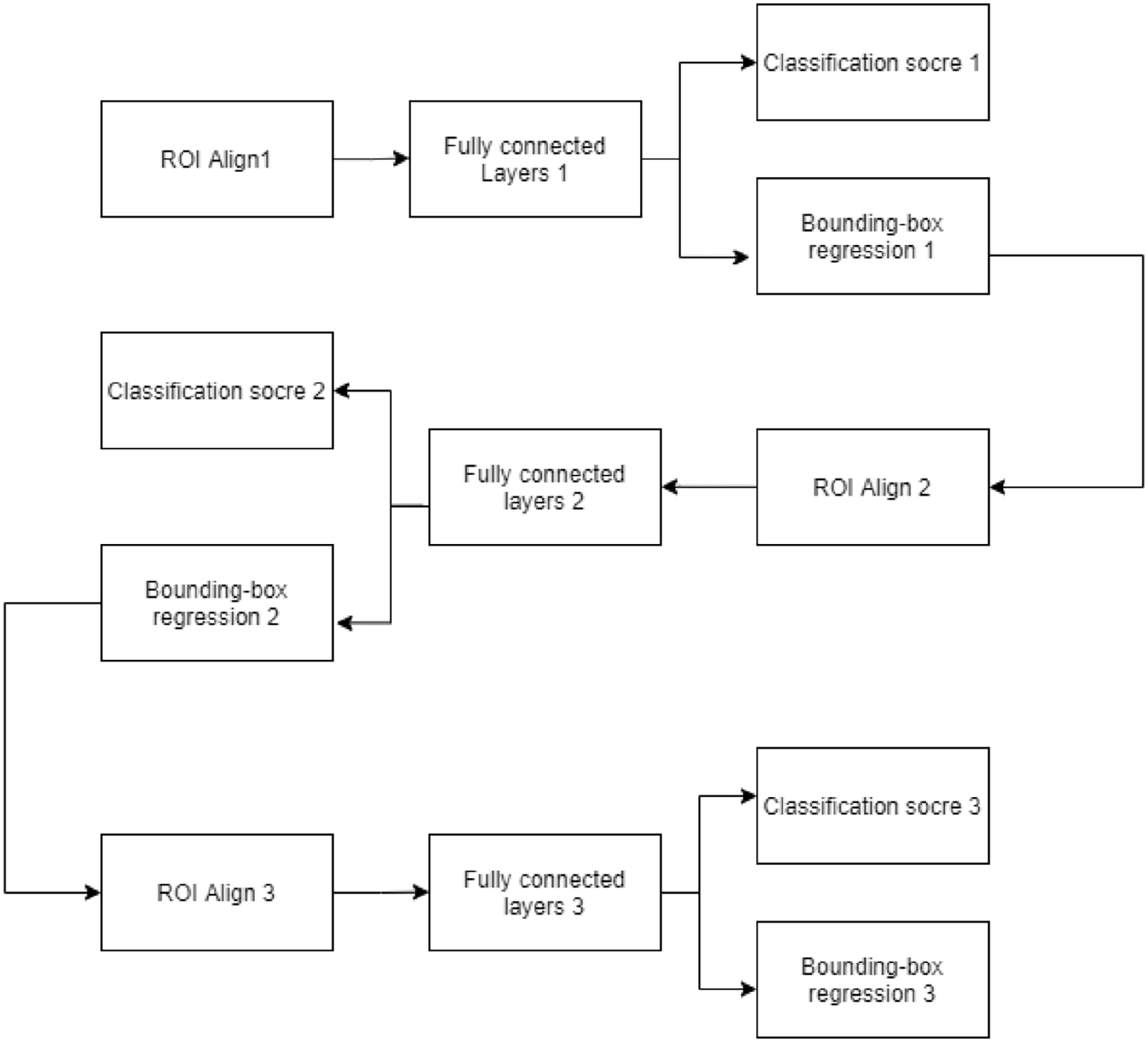
Structure of three stage Cascade module in this paper.

The Cascaded bounding box regression is composed of special regressors in each Cascaded stage, that is

f (x, b) = f_{T} \circ f_{T - 1} \circ \dots \circ f_{1} (x, b)

(7)

Where T represents the stage of Cascade, $f_{T}$ , $f_{T - 1}$ , $f_{1}$ represents the regressor of each stage,x represents the image batch and b represents the candidate box.

The loss expression of improved Cascade Faster R-CNN is as follows,

L (x^{t}, g) = L_{c l c} (h_{t} (x^{t}), y^{t}) + λ [y^{t} \geq 1] L_{l o c} (f_{t} (x^{t}, b^{t}), g)

(8)

Where $h_{t}$ represents the classifier, $f_{t}$ represents the regressor, $u^{t} > u^{t - 1}$ represents the IOU threshold, $b^{t} = f_{t - 1} (x^{t - 1}, b^{t - 1})$ , $g$ is the true value box of $x^{t}$ , $λ = 1$ represents weighing coefficient, [•] represents index function, $y^{t}$ represents $u^{t}$ label given by $x^{t}$ , so that the detection performance of the model is improved layer by layer.

Transfer learning

The main idea of transfer learning is to transfer the parameters of the pre-trained model to the new model to facilitate the training of the new model. Since most of the data are correlated, the learned model parameters can be shared with the new model through transfer learning, so as to improve the training speed and learning efficiency, rather than learning from scratch. In deep learning, in order to train a robust model, it is necessary to have the same distribution and independent sample sets, which is almost difficult to achieve in real life. ImageNet is a collection of millions of data sets that researchers have spent a lot of time and money collecting, mostly images of common objects in nature. Therefore, the transfer learning method is adopted in this paper. Pre-trained Imagenet is used to initialize the model, pre-trained weights are loaded, and only full-connection layer parameters are trained, namely Fine Tuning (FT), to solve the problems of lack of data samples and weak generalization ability.

Experiment and result analysis

This paper introduces transfer learning and improves the Faster R-CNN network using ResNet50 to detect fabric defects. The hardware environment of the experiment is an Intel (R) Core (TM) i7-10750H CPU. The PyTorch and TensorFlow deep learning frameworks are built under a windows 10 operating system. The steps of the developed software are as follows. (1) Preprocess the dataset and expand it through data augmentation. (2) Determine the experimental judgment index. (3) Select the weight transfer learning corresponding to the ResNet50 model to initialize the parameters of the improved algorithm model. Then, input the defect images into the CNN for training. (4) Identify defect types in the test sets using trained models. The software flowchart is shown in Figure 7.

Figure 7.

Software flowchart for the fabric detection algorithm.

Data preprocessing

The dataset is taken from actual scenes in a textile factory in Zhejiang Province. A total of 2119 images of untextured gray fabric and checked gray fabric were presented in yellow, black, black and white, blue and white, dark gray, dark red, gray, and white. The defect types include ribbon yarn, broken yarn, cotton ball, holes, yarn shedding, and stains with approximately 300 pictures for each defect type. The images are manually classified by experienced cloth inspectors. The resolution of each image is 512 × 512, and LabelImg is used to manually label the defect images and generate the corresponding xml format information file, which indicates the category and location information of the defect. The defect images were divided into training and validation sets at a 1:1 ratio, and the improved model was imported for training. Example images of the dataset for each defect type are shown in Figure 8.

Figure 8.

Defect samples in the dataset: (a1) ribbon yarn, (b1), broken yarn, (c1) cotton ball, (d1) hole, (e1) yarn shedding, (f1) stain, (a2) ribbon yarn, (b2) broken yarn, (c2) cotton ball, (d2) hole, (e2) yarn shedding, and (f2) stain.

Due to the small number of image samples collected, there is limited sample diversity. Therefore, before training the model, it is necessary to preprocess the training dataset and use the expanded dataset to improve both the accuracy of defect detection and the model robustness. If the images are only enlarged and narrowed, corresponding details will be lost. Thus, image augmentation operations are needed to increase the amount of contained information. The dataset is expanded by mirroring, rotations, exposure, and other operations to increase the number of images. Example images after data enhancement are shown in Figure 9.

Figure 9.

Example images after data augmentation: (a) mirror reflection, (b) rotation, and (c) exposure.

After data enhancement, the number of fabric image samples was expanded to 6357, including 1275 with yarn defects, 924 with yarn breaking defects, 552 with cotton ball defects, 336 with hole defects, 2004 with yarn shedding defects and 1266 with stain defects. It was divided into training set and verification set in 1:1 ratio, and the improved model was imported for training.

Determination of judgment index

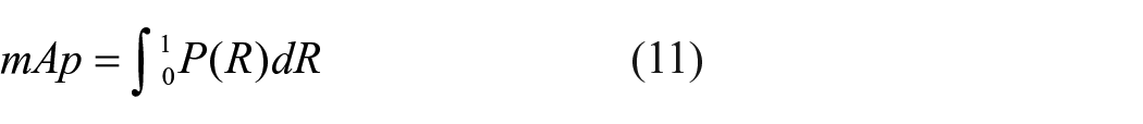
In the experiment, mean average precision (mAp) and verification accuracy are used as the judgment indexes for the model. Mean average precision represents the average value of AP, where AP represents the average precision of all classes in the dataset. F1 represents the harmonic average of recall and precision, that is, the recall and precision are evaluated together. The calculation process for precision, mAp and F1 are as follows.

Suppose that there are only two categories in the classification objectives defined as positive and negative. (1) True positive (TP) is the number of instances samples correctly divided into positive cases, that is, the number of samples that are positive and positively detected by the classifier. (2) False positive (FP) is the number of samples incorrectly divided into positive cases, that is, the number of samples that are negative but classified as positive. (3) False negative (FN) is the number of samples incorrectly classified as negative, that is, the number of samples that are actually positive but are classified as negative. (4) True negative (TN) is the number of samples that are correctly divided into negative cases, that is, the number of instances that are negative cases and classified as negative. Recall represents the proportion of samples predicted to be positive among all positive samples. Then, in equations (9) and (10), P and R represent the precision and recall, respectively, as:

p r e c i s i o n = \frac{T P}{T P + F P}

(9)

r e c a l l = \frac{T P}{T P + F N}

(10)

m A p = \int_{0}^{1} P (R) d R

(11)

F 1 = \frac{2}{\frac{1}{P} + \frac{1}{R}} = 2 \times \frac{P \times R}{P + R}

(12)

The loss value is also an important index to evaluate the quality of the model. For a specific sample, the loss represents the gap between the predicted value from the model and the real value. A smaller gap ideally gives a better-predicted value that is equal to the real value. A smaller loss gives a better model robustness.

Model training and test results analysis

Performance comparison of Faster R-CNN algorithm with different configurations

To verify the performance of the proposed defect detection system, the dataset is used to train the Faster R-CNN network in which the mainstream ResNet50, ResNet101, VGG16, and Mobilenet are used as the backbones. These Faster R-CNN algorithms with different configurations are shown in Table 3, where the Faster R-CNN (1) represents the VGG16 and introduces the ROI align, Faster R-CNN (2) represents the mobilenet and introduces the ROI align, Faster R-CNN (3) represents the ResNet101, and Faster R-CNN (4) represents the ResNet50. Faster R-CNN (5) represents the Faster R-CNN based on ResNet50 in which the FPN and ROI Align are introduced. The improved algorithm of this paper (Cascade Faster R-CNN) represents the Cascade Faster R-CNN based on ResNet50 in which the FPN and ROI Align are introduced.

Table 3.

Faster R-CNN algorithms with different configurations.

Experimental model	Backbone	ROI Align	ROI Pooling	FPN	Cascade
Faster R-CNN (1)	VGG16	√	×	×	×
Faster R-CNN (2)	Mobilenet	√	×	×	×
Faster R-CNN (3)	ResNet101	×	√	×	×
Faster R-CNN (4)	ResNet50	×	√	×	×
Faster R-CNN (5)	ResNet50	√	×	√	×
Improved algorithm of this paper (Cascade Faster R-CNN)	ResNet50	√	×	√	√

The number of epochs (processes in which the dataset passes through the neural network and returns once) in, Faster R-CNN (1), Faster R-CNN (2), Faster R-CNN (5) and the improved algorithm of this paper are 25, 15, 15, and 50, respectively. The learning rate (lr), loss rate (loss), and mAp are shown in Figures 9 to 12. In Figures 10(a), 11(a), 12(a), and 13(a), the abscissa represents the number of iterations, and the ordinate represents the loss rate and learning rate. In Figures 10(b), 11(b), 12(b), and 13(b), the abscissa represents the number of training epochs, and the ordinate represents the mean average accuracy (mAp). The learning rate is a super parameter that guides us how to use the gradient of the loss function to adjust the network weight in the gradient descent method. The loss rate is the error of the predicted value of the model. By minimizing the loss rate, the model can reach the convergence state.

Figure 10.

Performance of Faster R-CNN (1): (a) learning rate and loss rate and (b) mean average precision.

Figure 11.

Performance of Faster R-CNN (2): (a) learning rate and loss rate and (b) mean average precision.

Figure 12.

Performance of Faster R-CNN (5): (a) learning rate and loss rate and (b) mean average precision.

Figure 13.

Performance of the improved algorithm in this paper (Cascade Faster RCNN): (a) learning rate and loss rate and (b) mean average precision.

In terms of model learning rate (LR) and loss rate (loss), the green dotted line in Figure 10(a) shows that the Faster R-CNN (1) converges when training to the 20th group of data with a loss rate of 0.21. The green dotted line in Figure 11(a) shows that Faster R-CNN (2) converges when training to the 20th group of data with a loss rate of 0.12. The green dotted line in Figure 12(a) shows that Faster R-CNN (5) converges when training to the 12th group of data with a loss rate of 0.05. The green dotted line in Figure 13(a) shows that the improved algorithm of this paper converges when training to the 47th group of data with a loss rate of 0.005. The results suggest that the loss rate of the improved algorithm of this paper has reduced by 0.205, 0.105, and 0.045, respectively compared with Faster R-CNN (1), Faster R-CNN (2), and Faster R-CNN (5).

In terms of mAp, the red coordinate points in Figure 10(b) show that when the Faster R-CNN (1) is trained to the 20th group, the mAp reaches the highest value of 42.10% and remains stable. The red coordinate points in Figure 11(b) show that when the Faster R-CNN (2) is trained to the 20th group, the mAp reaches the highest value of 43.30% and remains stable. The red coordinate points in Figure 12(b) show that when the Faster R-CNN (5) is trained to the 12th group, the mAp reaches the highest value of 77.40% and remains stable. The red coordinate points in Figure 13(b) show that when the improved algorithm of this paper is trained to the 47th group, the mAp reaches the highest value of 94.73% and remains stable. Compared with the Faster R-CNN (1), Faster R-CNN (2), and Faster R-CNN (5), the mAp of the improved algorithm of this paper is enhanced by 52.63%, 51.43%, and 17.33%, respectively, with a higher accuracy.

In terms of training speed, calculate the quotient between the total training time of each model and epoch to obtain the average training time of each epoch, and then divide it by the total number of pictures in the data set to obtain the training speed of each model (i.e. the detection time of a single picture). Through calculation, the training speed of Faster R-CNN (1), Faster R-CNN (2), Faster R-CNN (3), Faster R-CNN (4), Faster R-CNN (5) and the improved algorithm of this paper is 0.4521, 0.3006, 0.3404, 0.3234, 0.3865, and 0.3650 s/piece, respectively. The comparison shows that the training speed of the improved algorithm of this paper is 0.0871 and 0.0215 s/piece higher than that of Faster R-CNN (1) and Faster R-CNN (5), and 0.0644, 0.0246, and 0.0416 s/piece lower than that of Faster R-CNN (2), Faster R-CNN (3), and Faster R-CNN (4).

Table 4 compares the performances of the Faster R-CNN (1), Faster R-CNN (2), Faster R-CNN (3), Faster R-CNN (4), Faster R-CNN (5) and the improved algorithm of this paper. The performances include the mAp and training speed (single picture detection time).

Table 4.

VThe performances of Faster R-CNN algorithms with different configurations.

Experimental model	mAp (mean average precision) (%)	Training speed (s. pieces⁻¹)
Faster R-CNN (1)	42. 10	0. 4521
Faster R-CNN (2)	43. 30	0. 3006
Faster R-CNN (3)	54. 96	0. 3404
Faster R-CNN (4)	66. 94	0. 3234
Faster R-CNN (5)	77. 40	0. 3865
Improved algorithm of this paper (Cascade Faster R-CNN)	94.73	0.3650

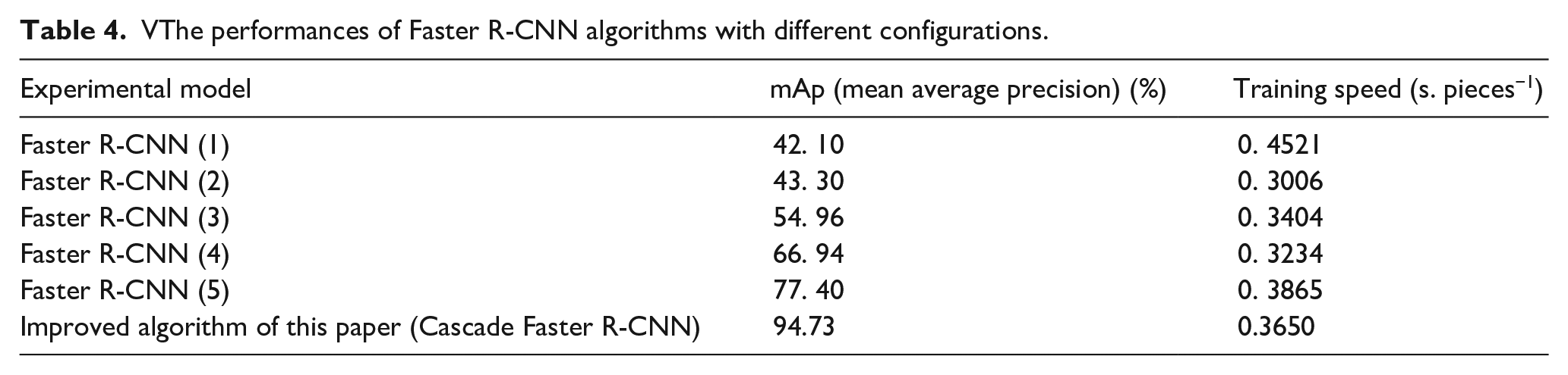
The table shows that compared with the Faster R-CNN (3) and Faster R-CNN (4), the mAp of the improved algorithm of this paper is enhanced by 39.77% and 27.79%, respectively. The training and experimental results show that compared with the Faster R-CNN (1), Faster R-CNN (2), Faster R-CNN (3), Faster R-CNN (4), and Faster R-CNN (5), the training speed of the improved algorithm of this paper (Cascade Faster R-CNN) is faster, the mAp is greatly improved. Therefore, the proposed fabric defect detection system based on transfer learning and the improved Faster R-CNN can better meet industrial needs.

Performance comparison of the improved algorithm with SSD and YOLOV3-tiny

SSD and YOLOV3-tiny algorithms are used to train the fabric defect data set in this paper,the detection results is shown in Table 5.

Table 5.

Performance Comparison of SSD andYOLOV3-tiny with Improved Algorithm.

Experimental model	mAp (Mean Average Precision) (%)	Training speed (s. pieces⁻¹)	Detection speed (fps)	F1
SSD	44.74	0.2300	27	0.364
YOLOV3-TINY	78.50	0.0930	48	0.619
Improved algorithm of this paper (Cascade Faster R-CNN)	94.73	0.3650	13	0.900

It can be seen from Table 5 that the mean average accuracy (mAp) of SSD and YOLOV3-tiny are 44.74% and 59.70%, respectively, the training speed is 0.2300 and 0.0930 s/piece, respectively, the detection speed is 27 and 48 fps, respectively, F1 is 0.364 and 0.619, respectively. The comparison shows that compared with SSD and YOLOV3-tiny, due to Cascade module is added to the improved algorithm in this paper, the amount of computation is increased, the detection speed and training speed is slightly decreased. However, in the case of insignificant speed reduction, mAp of the improved algorithm in this paper is obviously higher. Therefore, the improved algorithm proposed in this paper can effectively improve the performance of fabric defect detection system, and is more suitable for the actual production process.

Detection results of the improved algorithm

The improved algorithm of this paper is used to detect different types of defect images from textured gray cloth. Some detection results are shown in Figure 14. The defect types in Figure 14(a) to (f) are ribbon yarn, broken yarn, cotton ball, hole, yarn shedding, and stain, respectively.

Figure 14.

Detection results of the improved algorithm on different defect images: (a) ribbon yarn (a1: ribbon yarn 0.98 a2: ribbon yarn 0.97), (b) broken yarn (b1: broken yarn 0.99 b2: broken yarn 0.99), (c) cotton ball (c1: cotton ball 0.92 c2: cotton ball 0.90), (d) hole (d1: hole 0.91 d2: hole 0.96), (e) yarn shedding (e1: yarn shedding 0.94 e2: yarn shedding 0.89), and (f) stain (f1: stain 0.94 f2: stain 0.89).

It can be seen from Figure 14 that the improved algorithm of this paper can accurately locate defects of different sizes and predict each defect type. Therefore, the improved algorithm proposed in this paper effectively improves the performance of fabric defect detection system and strengthens the effect of network on fabric defect detection and classification.

In addition, the improved algorithm can also be used to detect textureless gray cloth. Before detection, the corresponding fabric image is imported into the training model, and the obtained weights for prediction are saved. In the textile fabric quality detection stage, the fabric image is taken in real-time through an industrial camera in conjunction with a supplementary light source. The supplementary light source prevents external interference and improves the collected image quality. The image is then imported into the industrial computer. Defective fabric can be quickly identified using the proposed model for analysis and prediction. The defect type can be accurately located and determined with a reduced false detection rate and missing detection rate relative to manual visual inspection, which realizes the automatic detection of fabric defects.

Conclusion

A fabric defect detection algorithm based on transfer learning and an improved Faster R-CNN is proposed. The dataset is first preprocessed, and the original Faster R-CNN is improved based on the idea of transfer learning where the feature extraction network is replaced by ResNet50, and the FPN is introduced. At the same time, the ROI pooling layer in the candidate box region extraction is replaced with the ROI Align layer for subsequent processing and predictions, and the Cascade module is added. Finally, the proposed model is compared and analyzed against current mainstream models. The results show that compared with the traditional algorithms, the proposed algorithm has the following advantages. The mean average precision reaches about 95% for six kinds of defects (ribbon yarn, broken yarn, cotton ball, hole, yarn shedding and stain), which is significantly improved compared with the original models. Compared with other Faster R-CNN algorithms with different configurations, the mAp is improved over a range of 15%–55%. Additionally, the convergence speed is faster during training. In summary, the improved algorithm performs well in terms of both accuracy and speed. The fabric defect detection shows a good effect for simple small target defects, which lays a foundation for further research on the influence of the fabric type, fabric texture, defect type, and size on the detection accuracy. At present, the algorithm proposed in this paper is still in the test stage. In the future, the algorithm can be further optimized in terms of training speed to better meet the actual fabric production needs.

Footnotes

Declaration of conflicting interests

The author(s) declared no potential conflicts of interest with respect to the research, authorship, and/or publication of this article.

Funding

The author(s) disclosed receipt of the following financial support for the research, authorship, and/or publication of this article: This paper is supported by Science and Technology Program of Hubei Province (No. 2019AEE011 No. 2018AAA036) and NSFC of China (No. 51175385)

ORCID iDs

Zhao Jia

Zheng Quan

References

Jiang

Liu

, et al. Fabric defect detection based on deep-handcrafted feature and weighted low-rank matrix representation. J Eng Fibers Fabr 2021; 16: 15589250211008453.

Guan

Shi

Fabric defect detection based on the saliency map construction of target-driven feature. J Text Inst 2018; 109(9): 1133–1142.

Yunan

Study on image analysis method of fabric defects. Shanghai: Donghua University, 1999.

Liu

Huo

, et al. DLSE-Net: A robust weakly supervised network for fabric defect detection. Displays 2021; 68: 102008.

Srinivasan

Dastoor

Radhakrishnaiah

, et al. FDAS: A knowledge-based framework for analysis of defects in woven textile structures. J Text Inst 1992; 83: 431–448.

Xie

Zhang

Fabric defect detection method combing image pyramid and direction template. IEEE Access 2019; 7: 182320–182334.

Tong

Wong

Kwong

CK.

Differential evolution-based optimal Gabor filter model for fabric inspection. Neurocomputing 2016; 173: 1386–1401.

Deotale

Sarode

TK.

Fabric defect detection adopting combined GLCM, Gabor wavelet features and random decision forest. 3D Research 2019; 10(1): 1–13.

Min

Cui

Xie

. Application of Gaussian mixture model on defect detection of print fabric. Text Res J 2015; 36(8): 94–98.

10.

Gao

Liu

, et al. Fabric defect detection based on biological vision modeling. IEEE Access 2018; 6: 27659–27670.

11.

Liang

, et al. Fabric defect detection via weighted low-rank decomposition and Laplacian regularization. J Eng Fibers Fabr 2020; 15: 1558925020957654.

12.

Yapi

Mejri

Allili

, et al. A learning-based approach for automatic defect detection in textile images. IFAC-PapersOnLine 2015; 48(3): 2423–2428.

13.

Basu

Chandra

Banerjee

, et al. Sub image based eigen fabrics method using multi-class SVM classifier for the detection and classification of defects in woven fabric. In: Third international conference on computing communication & networking technologies, Coimbatore, India, 26–28 July 2012, pp.1–6.

14.

Han

Statistic learning-based defect detection for twill fabrics. Int J Autom Comput 2010; 7(1): 86–94.

15.

Abdellah

Abdelmajid

Abdenabi

, et al. Defects detection and extraction in textile imageries using mathematical morphology and geometrical features. J Signal Process Theory Appl 2012; 1: 1–16.

16.

Xiaobo

Fabric defect detection of statistic aberration feature based on GMRF model. J Text Res 2013; 4: 26.

17.

Allili

Baaziz

Mejri

Texture modeling using contourlets and finite mixtures of generalized Gaussian distributions and applications. IEEE Trans Multimedia 2014; 16: 772–784.

18.

Dash

Behera

Dogra

, et al. Designing of marker-based augmented reality learning environment for kids using convolutional neural network architecture. Displays 2018; 55: 46–54.

19.

Ouyang

Hou

, et al. Fabric defect detection using activation layer embedded convolutional neural network. IEEE Access 2019; 7: 70130–70140.

20.

Bai

Chang

Nguyen

, et al. A high payload steganographic algorithm based on edge detection. Displays 2017; 46: 42–51.

21.

Gao

Zhai

Deng

, et al. Extended geometric models for stereoscopic 3D with vertical screen disparity. Displays 2020; 65: 42–51.

22.

Gao

Zhai

Yang

Stereoscopic 3D geometric distortions analyzed from the viewer’s point of view. PLoS One 2020; 15(10): e0240661.

23.

Liu

Wang

, et al. Fabric defect detection based on deep-feature and low-rank decomposition. J Eng Fibers Fabr 2020; 15: 155892502090302.

24.

Ming

Junfeng

Pengfei

Yarn dyed fabric defect identification using GAN and fast R-CNN. J Xi’an Univ Technol 2018; 32(6): 663–669.

25.

ChuanHua

Zhiqiang

Exuberant

, et al. Improved target precise location detection algorithm based on SSD. J Air Force Eng Univ 2018; 19(6): 73–78.

26.

Xie

, et al. Automatic defect detection and segmentation of tunnel surface using modified mask R-CNN. Measurement 2021; 178(4): 109316.

27.

Ngan

HYT

Pang

GKH

Yung

, et al. Wavelet based methods on patterned fabric defect detection. Pattern Recognit 2005; 38(4): 559–576.

28.

Zhao

Hao

, et al. A visual long-short-term memory based integrated CNN model for fabric defect image classification. Neurocomputing 2020; 380: 259–270.

29.

Zhao

Gui

Wang

. Fabric defect detection based on cascade faster R-CNN. In: CSAE 2020: The 4th international conference on computer science and application engineering, 2020.

30.

Shenbao

Tuimo

Decheng

Fabric defect detection based on improved Cascade R-CNN. Mod Text Technol 2021; 4(7): 81–87.

31.

Jing

Ren

Defect detection of printed fabric based on RGBAAM and Image Pyramid. Autex Res J 2021; 21(2): 135–141.

32.

Guanghui

Research on image annotation method based on transfer learning and depth convolution feature. Hangzhou: Zhejiang University of China, 2017.

33.

Junli

Kai

Yarn dyed fabric defect detection based on convolution neural network and transfer learning. Shanghai Text Technol 2019; 47(6): 52–56.

34.

Xiaona

Liang

Pengdi

Image change detection of panoramic blocks based on segnet network and transfer learning. J Chongqing Univ 2021; 155: 1–9.

35.

Yosinski

Clune

Bengio

, et al. How transferable are features in deep neural networks. In: Proceedings of the 27th international conference on neural information processing systems, Montreal, QC, 8–13 December 2014, pp.3320–3328. Cambridge: MIT Press.

36.

Lecun

Bottou

Bengio

, et al. Gradient-based learning applied to document recognition. Proc IEEE 1998; 86(11): 2278–2324.

37.

Xiong

Zhu

Sun

R, Application of transfer learning in continuous time series for aroma-ly detection in commercial aircraft flight data. In: IEEE Proceedings of 2018 IEEE international conferences on smart cloud (SmartCloud), New York, NY, 21–23 September 2018, pp.13–18. New York, NY: IEEE.

38.

Simonyan

Zisserman

. Very deep convolutional networks for large-scale image recognition. San Diego, CA: Published as a conference paper at ICLR, 2015. DOI: 10.48550/arXiv.1409.1556.

39.

Redmon Joseph

Divvala

, et al. You only look once: Unifified, real-time object detection. In: Conference on computer vision and pattern recognition, 2016, pp.779–788.

40.

Liu

Anguelov

Erhan

, et al. SSD: Single shot multibox detector. In: European conference on computer vision, 2016. Cham: Springer.

41.

Girshick

Donahue

Darrell

, et al. Rich feature hierarchies for accurate object detection and semantic segmentation. In: Computer vision and pattern recogonition, New Orleans, LA, 2014, pp.580–587. New York, NY: IEEE.

42.