Sage Journals: Discover world-class research

Abstract

The irregular cross section annular axis braided preform is modeled by using finite element simulation instead of geometric modeling. The braiding process is simulated by using a finite element software to obtain the yarn path. And the braided preform is modeled by using nine virtual fibers to form irregular cross section shape of yarn. Meanwhile, a modified vertical braiding machine is used to braid the actual preform, to compare with results from the simulation model. The results show that the simulation model is consistent with the actual braided preform, braiding angle is about 36°, and yarn spacing is about 6 mm. The finite element method can predict the yarn path more accurately without the need of complex analysis and derivation, especially when the irregular mandrel is used for braiding. In addition, the cross-section shape of yarn composed of virtual fibers can be used to achieve a more realistic simulation result. FEM is an efficient simulation method, and can also provide an effective basis in studies of the actual cross-sectional shape of yarn and the properties of its composite reinforcements.

Keywords

Braiding braid yarn mandrel cross-section

Introduction

Industrial braiding machine is usually divided into vertical braiding machine and horizontal braiding machine, working on the principle where multiple driving plates move two groups of yarn carriers in opposite directions to crisscross repeatedly on the eight-shaped track and the carriers allow the yarn to interlace on the mandrel.¹ One end of the yarn is driven by the carrier on the track board and another end is fixed on the mandrel through the braiding ring. The mandrel is usually linear and moves in a straight line under the traction of the driving device, and the yarns are interlaced and attached to the surface of the mandrel to form the braided preform, which can be used to process braided composites.² Braiding angle and yarn spacing are main parameters of braided preform.³

Many scholars studied the structure of braided preform usually by means of geometric modeling. Adanur⁴ developed a CAD model to describe the geometry of a 3D circular braid both externally and internally. Rawal et al.⁵ simulated various braided geometry structures based on different shapes of mandrels. Subsequently, the strands on complex-shaped mandrels including “bottle” and “funnel” were simulated.⁶ Alpyildiz⁷ studied geometrical modeling for tubular braids of different structures such as diamond, regular and triaxial braids.

Some scholars studied the braiding process on the irregular cross section mandrel and the structure of the braided preform. Kessels and Akkerman⁸ presented a fast and efficient model to predict the fiber angles on complex biaxially braided preforms. van Ravenhorst and Akkerman⁹ designed an inverse kinematics-based procedure for circular braiding machines on mandrels with complex 3D shapes including non-axisymmetric. Na developed a mathematical model to predict the braid pattern on arbitrary-shaped mandrels using the minimum path condition.¹⁰ These and many other studies described yarn path with geometric model,¹¹ so as to build a 3D model of braided preform.

In recent years, some scholars studied the braiding process through finite element simulation. Pickett et al.¹² used PAM-Solid software to simulate a two-dimensional braiding process and compared traditional analytical method with finite element method. Hans et al.¹³ combined Matlab, Abaqus, and VB to study the braiding process of mandrels in different shapes. Swery et al.¹⁴ studied a complete simulation method during the processing of braided composite part. Wu et al.¹⁵ studied numerical prediction method during the circular braiding process. Del Rosso et al.¹⁶ found that the use of single cylinders made of beam elements could be successfully employed for the virtual manufacture of open-mesh braids. Czichos et al.¹⁷ discretized the yarns into triangular shell elements to simulate the braiding process in the explicit finite-element code LS-DYNA. All these researches show that finite element method is effective for the simulation of the braiding process.

Compared with geometric modeling method, finite element method can predict yarn path more accurately, especially when an irregular mandrel is used for braiding. However, modeling of the braided preform has not been involved in the current studies using finite element method to simulate the braiding process. In this paper, a annular axis braided preform is modeled based on finite element simulation instead of geometric modeling. Firstly, the annular axis braiding process on the irregular cross section mandrel is simulated, to obtain the path of braid yarn from the post-processing of the simulation result. Secondly, different from previous studies, the braided preform is modeled by using virtual fibers to form irregular cross-sectional shape of yarn. Finally, the actual preform is braided by using a modified vertical braiding machine, to compare with the simulation model.

Design of mandrel

Irregular cross section annular axis braided preform studied in this paper is a composite preform obtained by 2D braiding on a closed annular axis mandrel connected from head to tail. The design of the closed annular axis mandrel is shown in Figure 1, and the inner radius of the closed ring of the mandrel is 255 mm.

Figure 1.

Closed annular axis mandrel.

The cross section of the mandrel is an irregular shape with a combination of curve and straight line, with larger angle at both intersections of the curve and the straight line, and at the bottom of the curve, as shown in Figure 2.

Figure 2.

Schematic diagram of the mandrel cross section.

Points A, B, and C in Figure 2 represent the three corners of the mandrel, and the surface of the mandrel is divided into three areas, so as to distinguish the surface of the mandrel when discussing braiding angle and yarn spacing in the following. It can be predicted that braid preform on this irregular cross section annular axis mandrel is different from braiding on the generally cylindrical linear mandrel. On the one hand, affected by the cross-sectional shape of the mandrel, the cross-sectional radius of the mandrel varies at different positions along the mandrel, so braiding angle of the yarn at different positions of the mandrel is also different. Especially when braiding to the three corners of the mandrel, the yarn will have a large bend. On the other hand, in the case of annular axis braiding, the axis direction of the mandrel changes constantly. If the influence of factors such as the difference of yarn tension and the change of yarn convergence area is taken into account, the structure of the braided preform may not always be in a regular symmetrical state. Therefore, for the irregular cross section annular axis braided preform, it is more complicated to deduce the path of braid yarn by using traditional geometric method, and it is more difficult to obtain accurate results without considering the yarn tension in the method.

Simulation of braiding process

In this paper, Abaqus/CAE 2018 finite element analysis software is used to simulate the annular axis braiding process. The basic assumptions are that the braid yarn is non-slipping on the mandrel, and the friction between the yarn and the braiding ring is not taken into account.¹⁸ Meanwhile, a spring is provided to connect with braid yarn, so that braid yarn always has a certain tension.¹⁹

According to the actual braiding, a finite element model mainly composed of braid yarn, braiding ring and annular axis mandrel is constructed. Since deformation of braiding ring and mandrel in the braiding process is negligible, discrete rigid elements are used to construct braiding ring and mandrel in finite element model, which also helps to ease the calculation. The shell shape is selected as the base feature of braiding ring and mandrel, and the 3D models of braiding ring and mandrel are obtained by sweeping their cross sections 360° around their own center. The cross section shape of mandrel is consistent with that shown in Figure 2. The diameter of mandrel is 510 mm, the diameter of braiding ring is 160 mm. The cross section of braiding ring is circular, and the cross section diameter is 10 mm. When constructing yarn model, the deformable type of 3D modeling space is selected, and the base feature is wire shape. Then each instance is imported in turn in the assembly module, and the instance type is set as dependent. The position of imported instance needs to be adjusted. Braid yarns are evenly distributed along the circumference of braiding ring. Each yarn passes through the braiding ring from the outside to the top and then moves down to the mandrel surface. The yarn convergence area is on the horizontal line of the mandrel center. The completed assembly model is shown in Figure 3.

Figure 3.

Schematic diagram of finite element model for annular axis braiding (1-mandrel, 2-braiding ring, 3-yarn, 4-spring).

Braid yarn is a key part of finite element model. The yarn shall not only be of high axial tensile strength, but also with certain flexibility. Therefore, it must be constructed with suitable element type. The truss element is connected by friction-free and freely rotatable hinges, usually divided into numerous smaller sections,^13,14 and its rigidity matrix K was shown in equation (1):

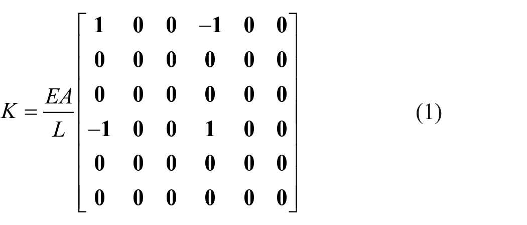
K = \frac{E A}{L} [\begin{matrix} 1 & 0 & 0 & - 1 & 0 & 0 \\ 0 & 0 & 0 & 0 & 0 & 0 \\ 0 & 0 & 0 & 0 & 0 & 0 \\ - 1 & 0 & 0 & 1 & 0 & 0 \\ 0 & 0 & 0 & 0 & 0 & 0 \\ 0 & 0 & 0 & 0 & 0 & 0 \end{matrix}]

(1)

Where E is the elastic modulus of yarn (MPa); L is the unit length (mm); A is the unit cross section area (mm²).

In the local coordinate system, the equilibrium equation of truss element was shown in equation (2):

K a + \frac{1}{2} A F_{0} e = F

(2)

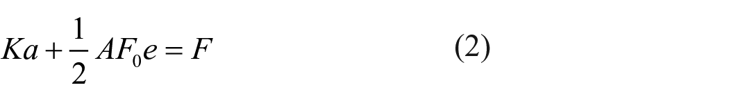
Where $F_{0}$ is the initial external force (N); F is the resultant force vector of node; $e = {[\begin{matrix} - 1 & 0 & 0 & 1 & 0 & 0 \end{matrix}]}^{T}$ ; a is the displacement vector of node.

Based on the idea of finite element discretization, if the braid yarn is discretized into several truss elements, the yarn model can maintain the flexibility of real yarn. As a result, truss element is used to construct the braid yarn model. In the element library, truss element in the explicit family is selected. The element type is T3D2, and each braid yarn is divided into 300 truss elements. The cross section of truss element is circular, the cross-sectional area is 0.1 mm², and the length of each element is 1 mm. Discrete rigid element in the explicit family is selected for the mandrel and braiding ring. The element type is R3D4.

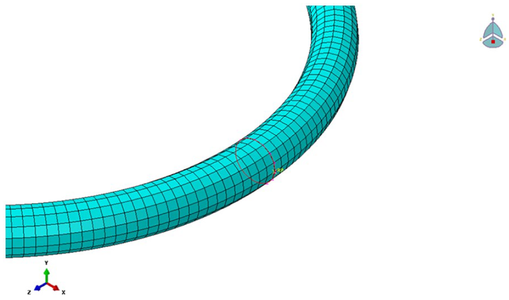
When meshing the mandrel and braiding ring, the sizing is controlled by setting the number of elements. Firstly, the mandrel section is divided into 30 elements along its contour line, and then the annular axis mandrel is divided into 200 elements along its circumference. The meshing diagram of the mandrel is shown in Figure 4.

Figure 4.

Meshing diagram of the mandrel.

By using the same method, the braiding ring is divided into 15 elements along the circumference of its section. The meshing diagram of braiding ring is shown in Figure 5.

Figure 5.

Meshing diagram of the braiding ring.

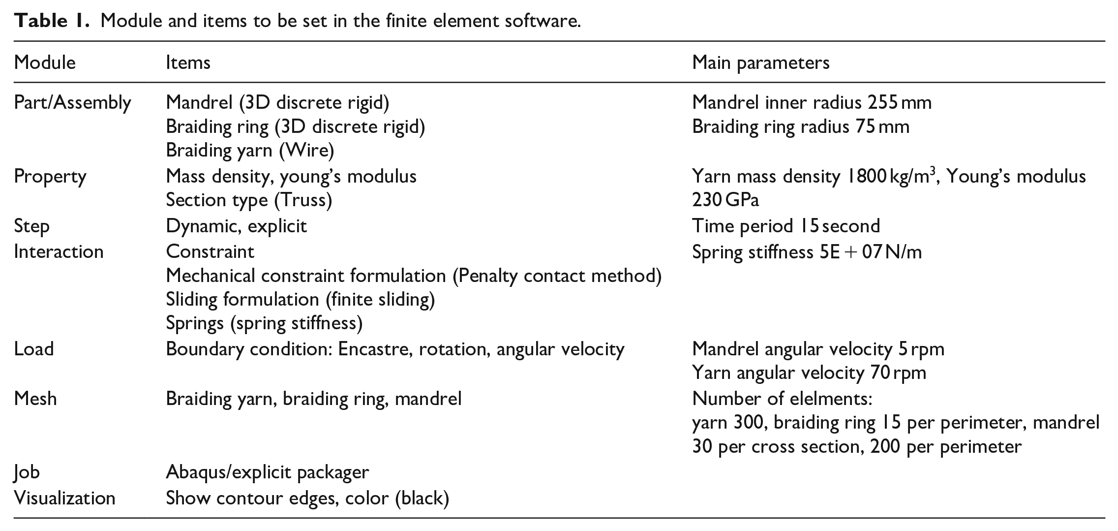
Reasonable boundary conditions need to be defined to simulate the braiding process. All degrees of freedom of the braiding ring are fixed. The displacement of the mandrel in three axes is constrained, and the rotation of the mandrel in X-axis and Y-axis is constrained. The mandrel is only allowed to rotate uniformly around its center in Z-axis, and the angular velocity is set at 5 rpm. One group of yarns rotate clockwise and another counterclockwise around Y-axis, the angular velocity is set at 70 rpm, and the rotation in X-axis and Z-axis is constrained. The braid yarn used in the simulation are of properties consistent with those of the real material, which is T700 carbon fiber yarn, with a elastic modulus of 230 GPa²⁰ and a density of 1800 kg/m³. One end of the braid yarn is bound to the mandrel, and the other end is connected by a spring to ensure that the braid yarn always has a certain tension. Spring stiffness is set at 5E + 07 N/m. The friction formulation between the yarn and the braiding ring is frictionless, and the friction formulation between the yarn and the mandrel is rough. Module and items to be set in the finite element software are shown in Table 1.

Table 1.

Module and items to be set in the finite element software.

Module	Items	Main parameters
Part/Assembly	Mandrel (3D discrete rigid) Braiding ring (3D discrete rigid) Braiding yarn (Wire)	Mandrel inner radius 255 mm Braiding ring radius 75 mm
Property	Mass density, young’s modulus Section type (Truss)	Yarn mass density 1800 kg/m³, Young’s modulus 230 GPa
Step	Dynamic, explicit	Time period 15 second
Interaction	Constraint Mechanical constraint formulation (Penalty contact method) Sliding formulation (finite sliding) Springs (spring stiffness)	Spring stiffness 5E + 07 N/m
Load	Boundary condition: Encastre, rotation, angular velocity	Mandrel angular velocity 5 rpm Yarn angular velocity 70 rpm
Mesh	Braiding yarn, braiding ring, mandrel	Number of elelments: yarn 300, braiding ring 15 per perimeter, mandrel 30 per cross section, 200 per perimeter
Job	Abaqus/explicit packager
Visualization	Show contour edges, color (black)

Explicit dynamic model was selected in the simulation, which can be used to deal with large geometric deformation and complex contact issues. The explicit central difference algorithm is suitable for nonlinear material with large deformation such as braid yarn.

Element node acceleration vector ${\overset{\cdot\cdot}{u}}_{t}$ could be represented by its displacement.

{\overset{\cdot\cdot}{u}}_{t} = \frac{1}{Δ t^{2}} (u_{t - Δ t} - 2 u_{t} + u_{t + Δ t})

(3)

Velocity vector ${\overset{\cdot}{u}}_{t}$ could be represented as follows:

{\overset{\cdot}{u}}_{t} = \frac{1}{2 Δ t} (- u_{t - Δ t} + u_{t + Δ t})

(4)

Where u is the node displacement vector, Dt is the time increment.

The motion equation at t time was shown in equation (5):

M {\overset{\cdot\cdot}{u}}_{t} + C {\overset{\cdot}{u}}_{t} + K u_{t} = {F_{e x t}}_{t}

(5)

Where M is the mass matrix, C is the damping matrix, $F_{e x t}$ is the external force vector of node.

Substitute equations (3) and (4) into equation (5) to realize the recurrence equation of the central difference method:

\begin{array}{l} (\frac{1}{Δ t^{2}} M + \frac{1}{2 Δ t} C) u_{t + Δ t} = {F_{e x t}}_{t} \\ - (K - \frac{2}{Δ t^{2}} M) u_{t} - (\frac{1}{Δ t^{2}} M - \frac{1}{2 Δ t} C) u_{t - Δ t} \end{array}

(6)

The result of $u_{t + Δ t}$ could be obtained based on the results of $u_{t - Δ t}$ and $u_{t}$ .

Penalty contact method is used in the mechanical constraint formulation, and the contact between the parts is defined as hard contact. In order to avoid possible contact penetration, large penalty stiffness is taken to produce a contact force in time, so as to prevent the further development of contact penetration.

After the job is submitted in the job manager, the simulation results of yarn path can be displayed in the visualization module. In the color and style settings of contour plot options, the yarn path can be displayed more clearly by setting thicker contour edges, as shown in Figure 6. After the two groups of braid yarns moving in opposite directions are interlaced, they are attached to the surface of the mandrel, and the complete path of the yarn can be easily observed by rotating, scaling, and other operations.

Figure 6.

Simulation result of annular axis braiding process.

The braid yarn always has a certain tension due to the spring, and different tension can be set for each yarn based on the damping coefficient of the spring. So finite element method is helpful to study the influence of yarn tension on the structure of braided preform and to further study the tension of braid yarn, while that cannot be reflected in traditional geometric modeling.

Modeling method of braided preform

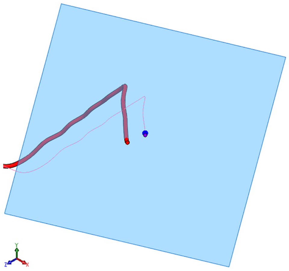
Through finite element method to simulate the annular axis braiding process, the yarn path of the braided preform can be obtained. In order to perform the modeling of the braided preform using the 3D design software, it is necessary to export the yarn path from the simulation results of the finite element software by some means and import it into the 3D design software. In Abaqus post-processing, the path of a deformed yarn is regenerated into a new part, and its inp file is viewed in plain text format, so as to find the 3D coordinate data corresponding to each node on this yarn. However, the inp file contains other information and data, so the 3D coordinate data of the yarn remains to be processed as necessary before being directly imported into the 3D design software. At this point, it is possible to use the edit function when importing the txt file into the Excel to delete the serial number of the 3D coordinate point data and other unnecessary codes in the inp file, and export a 3D coordinate data file that meets the requirements of the 3D design software. Then, in the 3D design software, import this file as a curve file, create a new curve formed by inputting 3D coordinate data, and finally reconstruct the yarn path after deformation, as shown in Figure 7. By repeating the steps above, all the paths of the braid yarns were obtained.

Figure 7.

Schematic diagram of deformed yarn path.

After obtaining the yarn path, it is also necessary to set the cross section of the yarn to complete the modeling of the braided preform. Since the yarn path is a three-dimensional curve, a new datum plane perpendicular to the direction of the yarn path should be created at the starting point of each yarn path, as shown in Figure 8. Then the yarn cross section is set on this datum plane, so as to ensure that the yarn cross section is always perpendicular to the yarn path and remains unchanged along the yarn path throughout the yarn model.

Figure 8.

Schematic diagram of new datum plane of yarn cross section.

For the modeling of the braided preform, the simplest method to set cross section is to use a constant circular as the cross section of the braid yarn. It is only required to draw a circular cross section and scan along the yarn path to obtain a 3D model of the braid yarn. Twenty-four braid yarns are modeled in sequence using this method, and the braided preform model with circular yarn cross section is obtained, as shown in Figure 9.

Figure 9.

Braided preform model with circular yarn cross section.

However, actual braided preforms often use carbon fiber yarns which are generally flat rather than with circular cross section. Therefore, when the circular yarn cross section is used for the modeling of the braided preform, the simulation result is not consistent with the actual situation of the braided preform. But if several virtual fibers are used to form the shape of the yarn cross section, it is closer to the actual situation of the braid yarn, and a more ideal simulation result can be realized.

Taking the starting point of the yarn path as the center, draw several circular virtual fiber cross sections to form a flat yarn cross section on the new datum plane of a yarn, as shown in Figure 10. A yarn consists of nine virtual fibers, each fiber has a circular cross section and a diameter of 0.2 mm. There is a certain interval and fluctuations between the virtual fibers. The horizontal distance between two virtual fibers is 0.25 mm, and the fluctuation in the vertical direction is 0.05 mm. By setting nine virtual fibers to form the yarn cross section in this way, the yarn cross section has a certain width and thickness, and it is not an absolutely regular rectangle. Meanwhile, the model will not be too complex because of nine virtual fibers.

Figure 10.

Yarn cross section shaped by virtual fibers.

With the yarn path and yarn cross section, it is possible to use the sweep function in the 3D design software to complete the modeling of the braided preform. The two groups of braid yarns with opposite direction of motion are set to different colors to obtain a braided preform simulation model with yarns composed of virtual fibers, as shown in Figure 11.

Figure 11.

Braided preform model with yarns composed of virtual fibers.

Compared with the braided preform simulation model with a circular yarn cross section as shown in Figure 9, the method of using virtual fibers to form the cross-sectional shape of the yarn can realize a simulation result closer to the actual braided preform. In addition, virtual fibers can be used to form more different cross-sectional shapes of yarns, so as to obtain more different simulation results.

Actual braided preform

Since ordinary braiding machines cannot directly braid on the closed annular axis mandrel, it is necessary to use a modified braiding machine and an additional mandrel drive device. In order to actually braid the above-mentioned simulated braided preform, a modified 24-carrier vertical braiding machine is used, as shown in Figure 12. Different from ordinary braiding machines, the track board of such a braiding machine can be opened and closed, so that the closed annular axis mandrel can enter and exit the convergence area of the braiding machine. Meanwhile, an additional mandrel drive device is used to transfer the rotation of the roller to the mandrel in the form of spokes connecting to the roller, so that the mandrel rotates around its own circle center to achieve continuous annular axis braiding. In addition, by using the braiding ring which can be opened and closed, the traditional braiding direction is changed. So that the mandrel drive device can pull the mandrel to move below the track board, which not only ensures that the convergence area is perpendicular to the track board, but also solves the problem of space limitation caused by finite diameter of track board and the mandrel.

Figure 12.

Braiding machine using annular axis mandrel.

Before braiding, first put the annular axis mandrel on the mandrel drive device, then push the track board of the braiding machine outwards along the guide rail while opening the braiding ring, and next move the mandrel drive device to push the mandrel into the convergence area in the center of the track board. Then, push the track board back to the original position along the guide rail while closing the braiding ring, and then draw yarns from the yarn carrier. Yarns pass through the braiding ring from bottom to top from the outside and then move downwards and are constrained to the mandrel surface before the braiding work commences. The braiding craft is consistent with the craft used in finite element simulation of the braiding process. The braided preform is drawn by the mandrel drive device to move below the track board. When the braiding is completed, the track board repeats the above actions to open outwards while the braiding ring is opened, and remove the mandrel drive device from which the mandrel is then removed to obtain the actual braided preform, as shown in Figure 13.

Figure 13.

Actual annular axis braided perform.

Whether it is the simulation model or the actual braided preform, braiding angle and yarn spacing can be measured by image analysis software.²¹ As shown in Figure 2, area 1 represents the area of the mandrel surface from point A to B, area 2 represents the area from point B to C, and area 3 represents the area from point C to A. According to the area division of the mandrel surface in Figure 2, images of the simulation model and the actual braided preform in these areas are obtained. Then, the angle and distance measurement tools in Image-Pro Plus software are used to measure the braiding angle and yarn spacing. In the measurement of the simulation model, the yarn path obtained from finite element simulation of the braiding process is used as the reference line to measure the braiding angle and yarn spacing, which is independent of the yarn cross section in the simulation model. And 20 data are measured for each group, and then the average value is taken to obtain the data comparison results, as shown in Table 2.

Table 2.

Comparison of braiding angle and yarn spacing between simulation model and actual braided perform.

Parameters	Braiding angle (°)				Yarn spacing (mm)
Parameters	Simulation	Std Dev	Actual	Std Dev	Simulation	Std Dev	Actual	Std Dev
Area 1 (point A-B)	34.0	6.26	35.1	2.89	5.8	1.78	5.3	1.04
Area 2 (point B-C)	39.6	4.67	37.9	2.71	6.1	1.47	6.5	2.19
Area 3 (point C-A)	34.0	4.99	35.8	3.46	5.5	1.84	5.3	1.54
Overall average	35.6	5.29	36.3	3.28	5.8	1.71	5.7	1.73

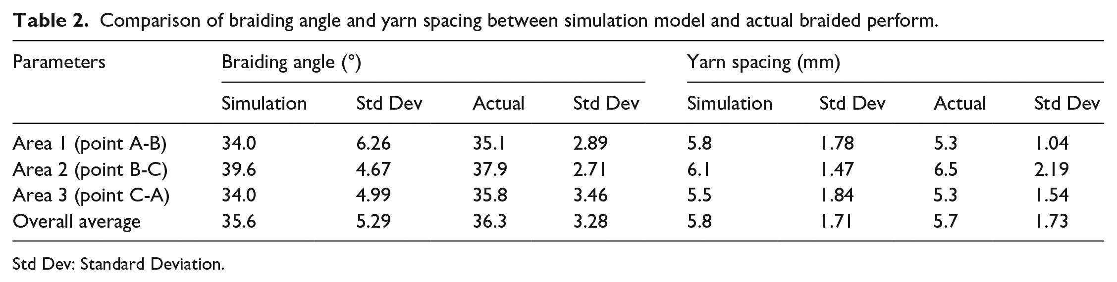
Std Dev: Standard Deviation.

Through comparison, it is found that the braiding angle and yarn spacing between the simulation model and the actual braided preform have relatively high goodness of fit. The yarn path in the simulation model is basically the same as the actual yarn path. After adopting the method of virtual fibers consisting of yarn cross section, the simulation model better reflects the real state where the flat carbon fiber yarns are attached to the mandrel surface in the actual braided preform.

Discussion

Through simulation the braiding process by using finite element method, the yarn path can be accurately obtained, and the 3D model of braided preform close to the actual situation can be constructed. However, this method uses truss element to construct braid yarn model, and its dynamic effect can be further studied.

The braided preform model based on finite element simulation can directly present the real shape of the braided preform, and further analyze its structure and performance. In particular, the changes of force and relative position of virtual fiber, as well as the resulting changes of cross-sectional shape of the yarn can be further studied, which may be one of the directions worth study in the future.

Conclusion

The modeling method of the irregular cross section annular axis braided preform by using finite element simulation can be used to obtain the yarn path without the need of complicated analysis and derivation, and the yarn path can be reflected more accurately. In addition, the yarn cross section shaped by virtual fibers can make the simulation results of the braided preform closer to the actual preform than the constant circular yarn cross section. The modeling method based on finite element simulation is an efficient simulation method for irregular cross section annular axis braided preform, and can also provide an effective basis for studies of the actual yarn cross-sectional shape and the properties of its composite reinforcements.

Footnotes

Declaration of conflicting interests

The author(s) declared no potential conflicts of interest with respect to the research, authorship, and/or publication of this article.

Funding

The author(s) received no financial support for the research, authorship, and/or publication of this article.

ORCID iD

Xi Wang

References

Potluri

Rawal

Rivaldi

, et al. Geometrical modelling and control of a triaxial braiding machine for producing 3D preforms. Compos A 2003; 34: 481–492.

Fouladi

Jafari Nedoushan

Prediction and optimization of yarn path in braiding of mandrels with flat faces. J Compos Mater 2018; 52: 581–592.

Shen

Branscomb

DJ.

A general approach to fast prototype the topology of braided structures. Int J Eng Sci 2018; 131: 40–60.

Adanur

3D structural simulation of tubular braided fabrics for net-shape composites. Text Res J 2000; 70: 297–303.

Rawal

Potluri

Steele

Geometrical modeling of the Yarn paths in three-dimensional braided structures. J Ind Text 2005; 35: 115–135.

Rawal

Gupta

Saraswat

, et al. Geometrical modeling of near-net shape braided preforms. Text Res J 2015; 85: 1055–1064.

Alpyildiz

3D geometrical modelling of tubular braids. Text Res J 2012; 82: 443–453.

Kessels

Akkerman

Prediction of the yarn trajectories on complex braided preforms. Compos A 2002; 33: 1073–1081.

van Ravenhorst

Akkerman

. Circular braiding take-up speed generation using inverse kinematics. Compos A 2014; 64: 147–158.

10.

Ahn

Jeon

S-Y

, et al. Prediction of the braid pattern on arbitrary-shaped mandrels using the minimum path condition. Compos Sci Technol 2014; 91: 30–37.

11.

Sheng

, et al. Mathematical and geometrical modeling of braided ropes bent over a sheave. J Eng Fibers Fabr 2020; 15: 155892502093972.

12.

Pickett

Erber

von Reden

, et al. Comparison of analytical and finite element simulation of 2D braiding. Plast Rubber Compos 2009; 38: 387–395.

13.

Hans

Cichosz

Brand

, et al. Finite element simulation of the braiding process for arbitrary mandrel shapes. Compos A 2015; 77: 124–132.

14.

Swery

Hans

Bultez

, et al. Complete simulation process chain for the manufacturing of braided composite parts. Compos A 2017; 102: 378–390.

15.

Shu

Kyosev

, et al. Numerical prediction methodology for tow orientation on irregular mandrels with constant cross-sections. J Compos Mater 2019; 53: 1067–1078.

16.

Del Rosso

Iannucci

Curtis

. Finite element simulation of the braiding process. Mech Adv Mater Mod Process 2019; 5: 1.

17.

Czichos

Bareiro

Pickett

, et al. Experimental and numerical studies of process variabilities in biaxial carbon fiber braids. Int J Mater Forming 2021; 14: 39–54.

18.

Zhang

Meng

, et al. Modeling and analysis of friction in end-face/inner-face circular braiding processes. J Text Inst 2018; 109: 1400–1408.

19.

Zhang

Meng

, et al. Tension modeling and analysis of braiding carriers during radial-direction and axial-direction braiding. J Text Inst 2019; 110: 1190–1201.

20.

Geng

, et al. Effect of thermal cycles on the thermal expansion behavior of T700 carbon fiber bundles. Chem Res Chin Univ 2018; 34: 451–456.

21.

Hajrasouliha

Nedoushan

Sheikhzadeh

, et al. Theoretical and experimental study of braid pattern in mandrels with arbitrary cross-sections. J Compos Mater 2018; 52: 4009–4022.

Modeling method of irregular cross section annular axis braided preform based on finite element simulation

Abstract

Keywords

Introduction

Design of mandrel

Simulation of braiding process

Modeling method of braided preform

Actual braided preform

Discussion

Conclusion

Footnotes

Declaration of conflicting interests

Funding

ORCID iD

References