
Abstract
Wool fiber and cashmere fiber are similar in physical and morphological characteristics. Thus, the identification of these two fibers has always been a challenging proposition. This study identifies five kinds of cashmere and wool fibers using a convolutional neural network model. To this end, image preprocessing was first performed. Then, following the VGGNet model, a convolutional neural network with 13 weight layers was established. A dataset with 50,000 fiber images was prepared for training and testing this newly established model. In the classification layer of the model, softmax regression was used to calculate the probability value of the input fiber image for each category, and the category with the highest probability value was selected as the prediction category of the fiber. In this experiment, the total identification accuracy of samples in the test set is close to 93%. Among these five fibers, Mongolian brown cashmere has the highest identification accuracy, reaching 99.7%. The identification accuracy of Chinese white cashmere is the lowest at 86.4%. Experimental results show that our model is an effective approach to the identification of multi-classification fiber.
Introduction
Cashmere, mohair, yak hair, camel hair, and alpaca wool are called special animal fibers. Among these fibers, characterized by its smoothness, softness, and luster, cashmere is the most popular animal fiber in the textile industry. Cashmere fiber comes from Kashmir goats and wool comes from sheep. Both kinds of fiber are composed of α-keratin, with an outer surface of overlapping cuticle cells. 1 Wool fiber and cashmere fiber are similar in their physical and morphological composite structure. As a high-grade textile material, however, cashmere is much more expensive than wool. False declarations and adulterations of wool are becoming a common practice by some manufacturers. Therefore, being able to distinguish between cashmere and wool is important. In the past few decades, many methods have been proposed for identifying cashmere and wool fibers. These methods include optical microscopy, scanning electron microscopy (SEM), near-infrared spectroscopy (NIRS), DNA analysis, image processing, and computer vision. 2 At present, optical microscopy is the most common identification method due to its low cost and easy operation, being widely used by enterprises and in quality and commodity inspections. 3 However, the identification accuracy of this method depends largely on the subjective experience of the operators, requires inspectors to have rich practical experience, and often results in discrepancies in the identification results among inspectors. The detection process is tedious, time-consuming, and has poor repeatability. 2 In addition, because the resolution is comparatively low, the images obtained by an optical microscope are not as clear as those of a scanning electron microscope, and characteristics such as the thickness of the scales on the fiber surface cannot be obtained.
SEM, with its high magnification (usually several thousand to tens of thousands), significant depth of field, strong stereo sense, and clear image acquisition, can analyze the microstructure of the fiber surface, offers easy-to-use image-processing technology, and provides the surface morphological parameters. For example, the thickness of scales on the fiber surface can be measured. Many studies have mentioned that the thickness of scales can better distinguish animal fibers. 4 However, scanning electron microscopes are very expensive. Usually, only large enterprises, universities, national inspection companies, and scientific research institutions can afford such equipment. In addition, the production of SEM samples is slow, and the detection cost is high.
In recent years, NIRS has been widely used in the textile field. Zoccola et al. 5 propose a method based on NIRS for identifying several kinds of animal fibers. DNA analysis has also attracted much attention. For example, Tang et al. 6 propose a method for identifying wool and cashmere based on mitochondrion DNA.
With the widespread use of computer technology, many scholars have begun to study the application of image-processing technology in fiber identification. 7 The use of image-processing techniques to identify fibers is somewhat similar to the microscope method described earlier, based on the image of the fiber under the microscope. Microscopy sometimes uses image-processing technology to help identify fibers but is based on manual identification. It only uses image-processing technology to measure a single parameter of the fiber (usually its diameter) to help staff make a judgment. Its main reliance depends on the subjective experience of the inspectors. Conversely, identification methods based on image processing, rather than subjective judgments, use image-processing technology to measure multiple geometric parameters of the fibers and employ a discriminant model to identify the fibers. A computer program rapidly completes the detection process. Shi et al.8,9 study the characteristics of the morphological parameters of cashmere and wool fiber surfaces in more detail.
Image-processing methods must measure various morphological parameters of the fiber surface; thus, these methods are limited by the quality of the micrographs. It is difficult to measure the height and area of fiber scales when the fiber image is blurred. Therefore, some scholars have explored the use of computer vision methods to decipher fiber scale patterns. Zhong et al. 2 propose an identification method based on projection curves.
During the last few years, deep learning technology, represented by convolutional neural networks (CNNs), has drawn significant attention in the field of computer vision. For example, CNN models have achieved good performance in image classification. This study mainly investigates the application of CNN models in fiber identification.
Research method
In this study, the process of fiber identification was divided into three steps. 10 In the first step, image preprocessing was performed. In the second step, following the VGGNet model, we established a CNN model called Fiber-net. Images of five kinds of wool and cashmere fibers were input into Fiber-net for training. In this step, we also adjusted the architecture and model parameters of the CNN. In the last step, the trained model is used to classify the fiber images in the test set.
Convolutional neural network (CNN)
CNNs are essentially feedforward networks that simulate the principle of the receptive field in biology.10–12 Although a variety of CNNs has emerged, in general, they are composed of pooling layers, convolutional layers, fully connected (FC) layers (FC layers can also be replaced by convolutional layers), input layers, and output layers. 13 In an input layer, an original image is input into a convolutional layer. In a convolutional layer, inputs are convolved with the learned weights to generate feature maps. The operation of a convolutional layer can be defined as
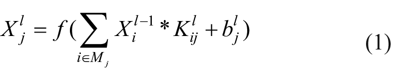
where
Pooling
The pooling layer is also called the aggregation layer and the down-sampling layer. Its main function is to reduce the dimension of the previous feature map and maintain the scale invariance. If the feature map is fed directly into the classifier or the next convolutional layer, the calculated amount may be very high, especially when the size of the feature map is relatively large. Thus, the pooling layer is essential. The operations of the pooling layer include average, max, and stochastic pooling. Take the commonly used max (average) pooling as an example. As shown in Figure 1, the pooling operation is performed on a four-block non-overlapping subregion (receptive field) to obtain a pooled feature map. The maximum value or average value is calculated for each subregion using a receptive field with a 2 × 2 window. 14

Illustrations of the pooling operation: (a) average pooling, and (b) max pooling.
Fully-connected network
In traditional CNNs, there is usually a connected network, which consists of several convolutional and pooling layers. Its main function is to perform high-level reasoning and interpret feature representations that are extracted from previous convolutional and pooling layers.15,16 In the CNN architecture for image classification tasks, the FC layer is usually placed at the end of the network, and the characteristics of its output are fed into the classifier. FC networks are not necessary for CNNs. Some CNNs use a 1 × 1 convolutional layer instead of FC network layers to reduce the number of parameters in the network.
VGGNet
VGGNet is a typical CNN, and it achieves excellent performance for ImageNet Large Scale Visual Recognition Challenge classification and localization tasks.
Input layer
VGGNet inputs are 224 × 224 RGB (referring to the red, green, and blue hues used) images. Thus, the preprocessing step includes converting the size of original images to 224 × 224 pixels and subtracting the average RGB value, which is calculated on all images in the training set, from each pixel.
Convolutional layer
Filters with a small receptive 3 × 3 pixel field are used in the convolutional layer. The convolution stride and the padding are set to one pixel.
Pooling layer
There are five pooling layers, which are placed behind some of the convolutional layers, in VGGNet. Maximum pooling is performed over a 2 × 2 pixel window and the stride is fixed to two pixels.
Fully connected (FC) layer
There are three FC layers, which follow a stack of convolutional layers and pooling layers, in VGGNet. Each of the first two FC layers contains 4096 channels. The third has 1000 channels, which represent 1000 categories. This is because the dataset used by VGGNet has 1000 categories for images.
Activation function
ReLU is applied as a simulation function to all weight layers except for FC layers.
Configurations
There are five CNNs with different configurations (A–E) in VGGNet. The five configurations vary only in depth. For example, configuration C has 16 weight layers, including three FC layers and 13 convolutional layers. Configuration E has 19 weight layers, including three FC layers and 16 convolutional layers. The number of channels in the convolutional layer doubles after each pooling layer, that is, from 64 to 512.
Experiment
Experimental setup
The samples include five kinds of fiber (four kinds of cashmere and one kind of wool), as shown in Figure 2: Mongolian brown cashmere, Chinese grey cashmere, Mongolian grey cashmere, Chinese white cashmere, and Chinese indigenous wool. The samples are dehaired cashmere fibers prepared by the Erdos Group. According to the standard GB/T10685-2007, the mean fiber diameter was measured using the projection microscope method. The values of mean fiber diameter of five fibers are: Mongolian brown cashmere 16.42 µm, Chinese grey cashmere 15.95 µm, Mongolian grey cashmere 16.36 µm, Chinese white cashmere 15.58 µm, and Chinese indigenous wool 17.23 µm, respectively. According to the standard GB18267-2013, the mean fiber length of was measured using the hand-arranging length method. The values of mean hand arranging length of five fibers are: Mongolian brown cashmere 37.7 mm, Chinese grey cashmere 36.3 mm, Mongolian grey cashmere 36.5 mm, Chinese white cashmere 34.2 mm, and Chinese indigenous wool 44.31 mm, respectively. Fiber images were captured with 10 × 50 magnification via an optical microscopic system (UVTEC CU-5), which was manufactured by Beijing UVTEC Company. Microscope images were stored in JPG format at 768 × 576 pixels in size. All images contain only one fiber and the majority of the fiber trunk was clearly captured. All fiber images had been prelabeled by seasoned experts. It is worthwhile mentioning that the total number of samples is equal to the total number of microscopic images. Therefore, the identification of animal fibers was transformed into the classification of fiber images.

Microscope images of five kinds of fiber: (a) Mongolian brown cashmere, (b) Chinese grey cashmere, (c) Mongolian grey cashmere, (d) Chinese white cashmere, and (e) Chinese indigenous wool.
A dataset with 50,000 fiber images was prepared. In this dataset, each kind of fiber has 10,000 images; thus, five kinds of fiber have 50,000 images in total. The dataset was split into three non-overlapping subsets: the training set to train the model, the test set to evaluate the model, and the validation set to adjust the hyperparameter of the model. We randomly took 5000 samples of the dataset as the test set (1000 samples of each kind of fiber), 40,000 samples of the dataset as the training set (8000 samples of each kind of fiber), and the remaining 5000 samples as the validation set. Figure 3 is the schematic diagram of the dataset split.

Splitting the dataset into the training set, validation set, and test set.
Referring to VGGNet, we established a CNN called Fiber-net to identify five kinds of cashmere and wool fibers in the dataset. The flowchart of the experiment is shown in Figure 4.

The flowchart of fiber identification.
The following is the process of training and testing Fiber-net. About 1.2 million images in 1000 categories from the ImageNet dataset were input into VGGNet for training, achieving a good classification result. As mentioned, our dataset was comprised of 50,000 fiber images in five categories; thus, far fewer than ImageNet. We first need to choose an appropriate CNN configuration to avoid possible overfitting.
In this experiment, the identification accuracy of fiber was defined as


where Ai (i = 1,2,3,4,5) is the identification accuracy of each kind of fiber, Ri represents the number of i-th kinds of fiber that were recognized correctly, Ti denotes the total number of i-th kinds of fiber, and At refers to the average accuracy of all kinds of fiber.
We first tried to classify the fiber dataset using four CNN configurations (A, B, D, and E) in VGGNet. The weight layers in these four configurations are 11, 13, 16, and 19, respectively. The fiber images were input into the four CNNs for training and testing. The recognition results of these CNNs were compared, as shown in Figure 5.
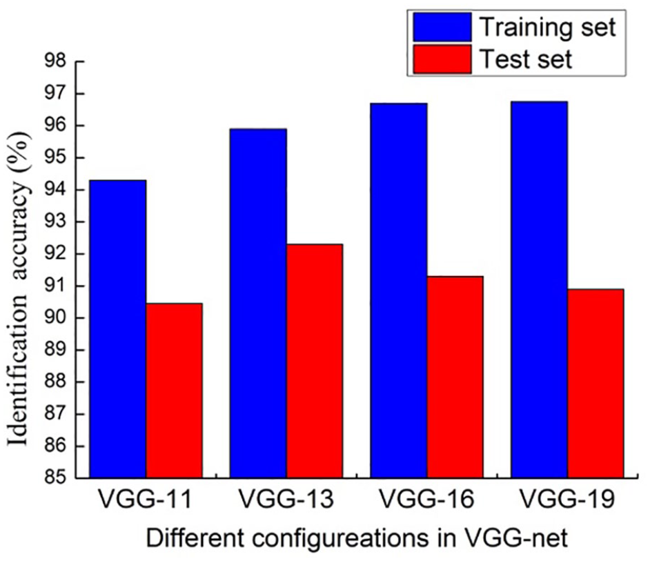
The identification accuracy of different configurations in VGGNet.
As shown in Figure 5, we found that, with an increase in the number of network layers, the identification accuracy of the training set increases, and the identification accuracy of VGG-13 (VGGNet configuration B) is the highest in the test set. The reason may be that when the sample size is not large enough, a deep network is more prone to overfitting. Therefore, we initially decided to use a CNN with 13 or 14 weight layers. Next, we adjusted the number of convolution kernels per layer according to VGG-13. We tried different CNN configurations, as shown in Table 1.
CNN configurations.

Then, the fiber images were fed into the CNNs for training and testing, and the identification accuracy of these CNNs are shown in Figure 6.

Identification accuracy of different CNN configuration.
From Figure 6, it can be seen that the CNNs in configurations 3 and 4 achieved higher identification accuracy in the test set. In Table 1, it can be seen that there are fewer convolution kernels used in the last two convolutional layers of CNN configuration 4, and the number of the first two FC layers is also less than that of configuration 3. Therefore, we choose configuration 4 as the fiber identification model and named it Fiber-net. Figure 7 shows a comparison of the classic CNN model VGG-16 and Fiber-net model architecture. The number of nodes in the last FC layer was set according to the number of classifications. The fiber dataset contains five kinds of fiber, so the number of nodes in the last FC layer was set to five.

VGG-16 and Fiber-net: (a) VGG-16, and (b) Fiber-net.
Five kinds of cashmere and wool fiber images from the dataset were fed into the Fiber-net model, and the total identification accuracy was 92.74%. Among them, Mongolian brown cashmere had the highest identification accuracy at 99.7%, followed by Chinese indigenous wool with an identification accuracy of 96.7%. The identification accuracy of Chinese white cashmere was relatively low at 86.4%, whereas Chinese grey cashmere and Mongolian grey cashmere were 90.8% and 89.8%, respectively. Experimental results show that our model can solve the problem of multi-classification fiber recognition.
Training and testing
In our experiment, the training procedure of the CNN is similar to that of VGGNet (except for the initialization of the network weights). We take Fiber-net as an example to introduce the training process. In image preprocessing, the size of the fiber images was first reduced to 256 × 256 pixels, and then the reduced images were randomly cropped to 224 × 224 pixel sizes. Mini-batch gradient descent with an Adam algorithm was applied during the training procedure. After tuning the model, its hyper-parameters were set. The batch size was set to 32. The learning rate was initially set to 0.001. Exponential decay rates for the first and second moment estimates were set to 0.99 and 0.999, respectively. The stochastic objective function with the epsilon parameter, a small constant for numerical stability, was set to 10−8. Dropout regularization was applied to the first two FC layers and the dropout ratio was set to 0.5. In total, the learning rate was stopped after 700 K iterations. Through TensorBoard, a visualization tool in TensorFlow, it is observed that when the model is trained to 600 K iterations, the loss is close to zero and tends to be stable. The change of the learning rate and loss during the Fiber-net training is shown in Figure 8. In the trained model, the identification accuracy of the training set and test set were 95.7% and 92.74%, respectively.
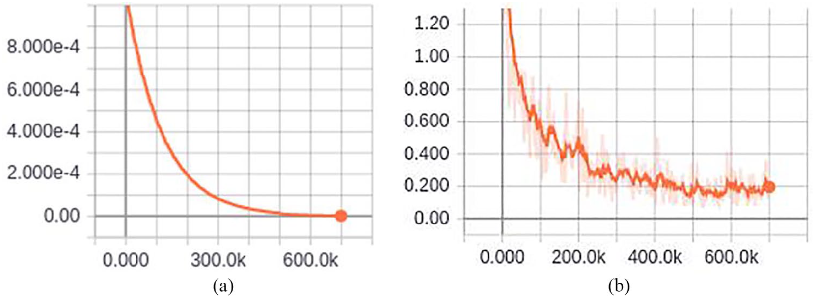
Learning rate and loss: (a) learning rate, and (b) loss. The x-axis represents steps, which is the number of iterations during training.
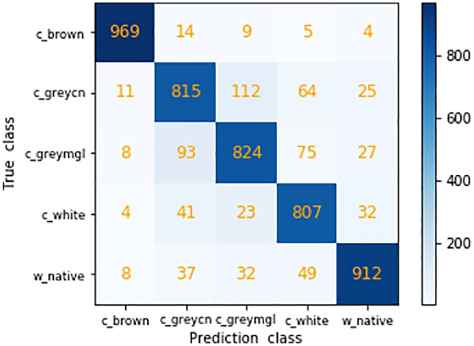
The confusion matrix, a specific table layout, is a summary of prediction results for a classification task. It provides a visualization of a model’s performance. The rows and columns of the confusion matrix correspond to the predicted class and the actual class, respectively. The number of correct and incorrect predictions are summarized with count values and broken down by each class. The confusion matrix for the five fiber classifications shows the number and types of errors being made by the model, as illustrated in Figure 9.

Confusion matrix of Fiber-net classification results.
In the experiment, c_brown, c_greycn, c_greymgl, c_white, and w_native were used to represent Mongolian brown cashmere, Chinese grey cashmere, Mongolian grey cashmere, Chinese white cashmere, and Chinese indigenous wool, respectively. Taking Mongolian grey cashmere as an example, each cell in row 1 represents the number of Mongolian brown cashmere images that were predicted to be in the various fiber class. It can be seen in Figure 9 that one of 1000 Mongolian brown cashmere images in the test set was predicted to be Chinese white cashmere, two images were predicted to be Chinese indigenous wool, and the remaining 997 images were predicted correctly. Because the surface of Mongolian brown cashmere is brown, the feature is obvious, so its identification accuracy is highest. Moreover, the identification accuracy of Chinese indigenous wool (row 5) is also relatively high, and only 33 images were predicted incorrectly. In comparison, the identification accuracy of the other three kinds of fiber was low.
As shown in Figure 9, Chinese white cashmere has the lowest recognition accuracy. Some white cashmere fibers were identified as Chinese grey cashmere, Mongolian grey cashmere and Chinese indigenous wool. In our previous study, we proposed a fiber identification method based on the BoW (Bag of Words) model, which is also based on the visual characteristics of fiber images. 17 For comparison, we use the BoW model to identify these fibers. The two methods have a similar trend, with many white cashmere fibers being misjudged by models as grey cashmere and wool fibers. Based on these conditions, we believe that white cashmere has visual characteristics similar to grey cashmere and Chinese indigenous wool, so it is easy to be misjudged. The confusion matrix of the BoW model classification results is shown in Figure 10.
Confusion matrix of the BoW classification results.
Predicted probability of fiber
We further observed the prediction information of the model for each sample using the Fiber-net model as follows. In the classification layer, softmax regression was used to calculate the probability value of the input fiber image for each category, and the category with the highest probability value was selected as the prediction category of the fiber. We then visualized the prediction probability of the fiber. Figure 11 shows the predicted results of Mongolian brown cashmere.

Prediction of Mongolian brown cashmere.
In the experiment, the fiber image file was named with the corresponding category string as a prefix. For example, the file name “c_brown_g8_398” of the test image indicates that the true category of the fiber is Mongolian brown cashmere. In Figure 10, the fiber image at the upper left was scaled to 256 × 256 from the original image, and the fiber image on the upper right was obtained by preprocessing the left image. The “Prediction class” tag in the bottom image is followed by the file name of the fiber image “c_brown_g8_398.jpg.” The bar chart in Figure 10 is the model’s prediction of the fiber image category. The highest prediction category is placed at the top. As can be seen from Figure 11, the probability that the image is predicted to be Mongolian brown cashmere is about 0.9, and the probability that it is Chinese grey cashmere is about 0.1. The category with the highest probability is used as the prediction category of the model. According to the prefix of the image name, it is found that the true category of the fiber is “c_brown” (Mongolian brown cashmere), which is consistent with the prediction results. Figure 12 lists the predictions of the Fiber-net model for randomly selected Chinese grey cashmere, Mongolian grey cashmere, Chinese white cashmere, and Chinese indigenous wool images.

Predictions of fibers: (a) Chinese grey cashmere, (b) Mongolian grey cashmere, (c) Chinese white cashmere, and (d) Chinese indigenous wool.
Conclusion
The identification of cashmere and wool fibers has been a challenging problem for a long time. The method presented in this paper offers a solution to this problem. In this method, a CNN model called Fiber-net was established to identify five kinds of fiber, and the total identification accuracy of the fibers in the test set was 92.27%. In our experiment, the confusion matrix was calculated. This provided not only the number of correct and incorrect predictions but also the types and number of errors made. Among the five kinds of fibers, Mongolian brown cashmere has the highest identification accuracy, while Chinese white cashmere has relatively low recognition accuracy. It can be seen from the confusion matrix that some of the white cashmere fibers was identified as grey cashmere and Chinese indigenous wool fibers. This is the first investigation to identify multiple categories of cashmere and wool fibers. This is also the first time that a large sample is used to evaluate the application of a CNN model in fiber identification. Experimental results show that proposed method can solve the problem of multi-classification fiber identification.
Footnotes
Acknowledgements
The authors would like to thank the anonymous reviewers for their carefulness and patience.
Declaration of conflicting interests
The author(s) declared no potential conflicts of interest with respect to the research, authorship, and/or publication of this article.
Funding
The author(s) disclosed receipt of the following financial support for the research, authorship, and/or publication of this article: This work is supported by the Key Technologies R&D Program of Henan Province under Grant No: 192102210135 and 212102210402, the Key Project of Institutions of Higher Learning in Henan Province under Grant No: 18A520010 and 20B520032, Xuchang University Research Fund Project under Grant No: 2020YB018.