Fabric defect recognition using optimized neural networks

Abstract

Fabric defect recognition is an important measure for quality control in a textile factory. This article utilizes a deep convolutional neural network to recognize defects in fabrics that have complicated textures. Although convolutional neural networks are very powerful, a large number of parameters consume considerable computation time and memory bandwidth. In real-world applications, however, the fabric defect recognition task needs to be carried out in a timely fashion on a computation-limited platform. To optimize a deep convolutional neural network, a novel method is introduced to reveal the input pattern that originally caused a specific activation in the network feature maps. Using this visualization technique, this study visualizes the features in a fully trained convolutional model and attempts to change the architecture of original neural network to reduce computational load. After a series of improvements, a new convolutional network is acquired that is more efficient to the fabric image feature extraction, and the computation load and the total number of parameters in the new network is 23% and 8.9%, respectively, of the original model. The proposed neural network is specifically tailored for fabric defect recognition in resource-constrained environments. All of the source code and pretrained models are available online at https://github.com/ZCmeteor.

Introduction

The cost of advanced textiles is often affected by fabric defects that represent a major problem to the garment industry. Therefore, automatic inspection systems are required by a textile manufacturer to maintain fabric quality. ¹ With the development of automation technology, increasingly more recognition and detection technologies based on computer vision are used in industrial production.^2,3 Traditionally, fabric defect inspection approaches were categorized into five groups: spectral methods, low-rank decomposition methods, model-based methods, statistical methods, and structural methods. ⁴ These fabric defect inspection approaches based on conventional computer vision have been developed for more than 10 years, especially scale-invariant feature transform (SIFT) ⁵ and histogram of oriented gradients (HOG). ⁶

At present, most of the traditional visual fabric defect detection algorithms utilize handcrafted features extracted from each fabric image patch to differentiate between defective regions and defect-free regions. Unfortunately, these conventional detection algorithms cannot accurately and efficiently recognize various types of fabric defects due to either the low discriminative ability of the extracted handcrafted features or their time-consuming sliding window strategy. Accordingly, conventional defect inspection approaches have been intensively focused on the plain and twill fabric, and their results tend to be unsatisfactory for complicated jacquard warp-knitted fabric. In addition, these conventional algorithms usually can not provide a general inspection capability. The performances of these conventional defect recognition algorithms heavily rely on the discriminative capability of handcrafted features extracted by each fabric image patch. However, at present, no unified handcrafted feature descriptor is appropriate for all types of fabric images. Thus, traditional fabric defect recognition algorithms are unable to achieve good performances on multiple textile types simultaneously. For industrial productions, there is no explicit guideline for choosing optimal defect inspection algorithms. As such, human expertise is the critical factor to the success of fabric defect inspection. It is laborious to provide a generic fabric defect inspection approaches that apply to wide range of fabrics. To address these shortcomings, a model with a generic feature extraction capability is needed to improve the existing automated recognition system.

As a predominant machine learning algorithm, deep learning has been rapidly developed and has gained considerable attention in recent years. Convolutional networks have demonstrated excellent performance in computer vision tasks, such as object recognition and target detection, since LeCun et al.’s ⁷ proposal in the early-1989. Krizhevsky et al. ⁸ showed record-beating performance on the ImageNet Large-Scale Visual Recognition Challenge classification benchmark in 2012. He et al. ⁹ demonstrated state-of-the-art performance on the Common Objects in Context (COCO) 2016 challenge 3 years ago. Most notably, just this year, Yang et al. ¹⁰ present a novel fully convolutional autoencoder approach that accurately segments various types of product surface defects based on a small number of defect-free product samples. This fully convolutional autoencoder achieves a precision of 92.0% while requiring only 82 milliseconds for 1920 × 1080 input image pixel. All the abovementioned results indicate that convolutional networks may be applied to the feature extraction of fabric images because of the predominant feature extraction characteristic of these congeneric networks.

However, there are some issues about applying convolutional networks to fabric defect recognition. First, convolutional neural models are both computational and memory intensive, and a large number of parameters consume considerable storage bandwidth. This disadvantage makes them difficult to deploy on field-programmable gate arrays and embedded systems with limited hardware resources. ¹¹ So this storage requirement may be harsh and even impossible in many industrial occasions. Second, current deep convolutional networks often have a very complex architecture for the sake of extracting advanced features in target images, which greatly increases the calculation expense and is not feasible in online fabric defect recognition. Convolutional networks usually have a good generalization ability, but this capability is unsuitable for special feature extraction occasions because there may be some parameter redundancies in a convolutional network for specific purposes. ¹²

To address these limitations, this article references a visualization technique as proposed by Zeiler and Fergus ¹³ that displays the input images that activate individual feature maps at any layers in the convolutional networks. This technique also allows researchers to investigate the evolution of invisible features and the diagnosis of potential problems in a convolutional model. A multilayered deconvolutional network is utilized to project the feature activities back to the input pixel space. Using these tools, this study explores the architecture of conventional convolutional networks and researches different configurations, discovering ones that outperform accuracy-wise conventional convolutional networks for fabric defect recognition, while the number of parameters and amount of calculation only accounts for 8.9% and 23%, respectively, of the original model.

Fabric defect recognition using VGG16

Model selection

This article chooses a convolutional network that has been widely used in recent years and utilizes it in fabric defect recognition experiments. The main advantages that convolutional model should possess are as follows: First, the model must ensure that the fabric defect recognition system has a high detection accuracy. Second, the model should have rapid running speed to facilitate real-time detection in industrial fields, because the profits of textile manufacturing enterprises are directly affected by their production efficiency. Third, the generalization ability of whole defect recognition system should be excellent owing to textile manufacturers do not have the capability to train a complete fabric defect recognition system, so the fully trained model should be suitable for as many types of cloth as possible.

It is not difficult to find some of the most advanced convolution models and apply them to fabric defect identification. However, the state-of-the-art network topology is usually too complex, and the spatial resolution of feature maps is aggressively reduced to increase the local receptive field. For instance, the residual neural network (ResNet) ¹⁴ has outstanding classification performance, but it has too many network layers, which makes it difficult to train or test. The whole model of GoogLeNet ¹⁵ has very few parameters but maintains a high classification accuracy. However, this model does not have fully connected layers, which leads to the lack of generalization ability. Thus, it needs to be separately trained when it is applied in various commercial fields.

At present, the Visual Geometry Group (VGG) ¹⁶ network has been widely applied in the commercial fields,^17–19 because of its excellent generalization capability and relatively simple structure (which uses filters with a very small receptive field in all layers). There are 16 weight layers in VGG16, which has 13 convolutional layers and 3 fully connected layers. The filter kernels use a very small 3 × 3 pixel window. The convolution stride is fixed to one, and the padding is 1 pixel for the 3 × 3 filters. All hidden layers are equipped with ReLU ⁸ nonlinearity. Spatial pooling is carried out by five max-pooling layers, which follow some of the convolutional layers. Max-pooling is performed over a 2 × 2 receptive field with stride two. The configuration of the fully connected layers is similar in conventional convolutional networks (e.g. AlexNet). Rather than using relatively larger receptive fields in the first convolutional layer (e.g. an 11 × 11 receptive field size with stride four in AlexNet), VGG uses a very small 3 × 3 filter size with stride one throughout the whole model, which is convolved with the input image at every pixel. The small filter size offers a number of benefits. First, this structure decreases the number of convolutional layer parameters (there are only 14.7-million parameters in the convolutional layers). Second, this structure incorporates more ReLU ⁸ nonlinearity layers instead of a single layer, which makes the decision function more discriminative. ²⁰

Development environment

At present, there are many development tool kits for deep learning, but they are mutually incompatible. Since 2015, TensorFlow, an open source library, has attracted increasing attention. TensorFlow is a machine learning toolkit that uses tensor flow graphs for numerical computations. The graph nodes symbolize mathematical operations, while the graph lines symbolize the multidimensional tensors that flow between them. ²¹ This flexible structure enables us to implement computation on multi-core central processing units (CPUs) or graphics processing units (GPUs) without rewriting code, which means that fabric defect recognition systems can be easily and conveniently implemented in industrial fields. TensorFlow is now far more influential than other machine learning toolkits, so we ported the original code^13,16 from Caffe ²² and implemented it in TensorFlow. The operating system is Windows 10, and the processors are two Intel Xeon(R) E5-2650-v4 CPUs and two Quadro M5000 GPUs. If there is no special explanation, all the experiments in this article run in this development environment.

Fine-tuning VGG16

The model structure we used was almost identical to the original VGG16. The only difference is that the number of channels in the last layer changed from 1000 to 2 (because it was only necessary to distinguish whether or not the defects are included in a fabric image). To make the model converge more quickly, we did not randomly initialize it, but instead used the pretrained parameters as the initial values in untrained model and then fine tuned it. In this section, we describe the details of fabric defect recognition model training and testing.

Training

In this article, the model training procedure generally follows Simonya and Zisserman. ¹⁶ The database we used was purchased from Xiamen Face++ Company for 0.25 US dollars per image. The fabric database is different from the common classic database because it contains much richer fabric images, as shown in Figure 1. Most of the materials have a complicated texture, which poses a great challenge to the defect recognition system. The fabric dataset has approximately 8000 fabric images in two categories (4000 are defective and 4000 are defect-free). We randomly selected 6000 images from the fabric database as training set and 2000 as testing set. (In training set, 3000 are defective and 3000 are defect-free. In testing set, 1000 are defective and 1000 are defect-free.) The initialization for the network parameters is important because poor initialization can stall learning due to the instability of stochastic gradient descent in a deep network. To combat poor initialization, we choose the parameters pretrained (https://github.com/) by ImageNet as the initial values in untrained model, then freeze the parameters in the first seven convolutional layers and only fine tune the last nine layers. The purpose of this freezing operation is not only to further improve the convergence rate of the model (only half of the parameters need to be trained) but also to make the model not prone to gradient explosion during training. ⁸ Because the anterior layers in a deep convolutional neural network only learn some contour features, such as boundaries, shapes, and colors, the anterior layers in same convolutional neural network have almost the same parameters, no matter what visual tasks are applied. ²³

Figure 1.

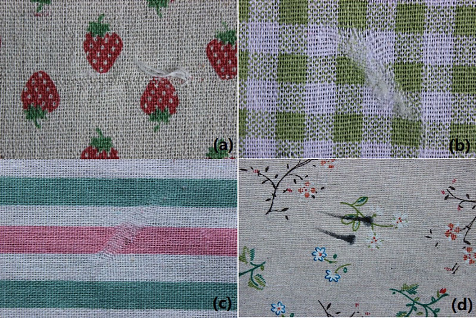
Some samples of the fabric defect images from our database: (a) missing yarn, (b) scratch defect, (c) twill flaw and (d) dye spot. All images in our database are true color images, and most of normal fabrics have complicated textures and patterns. These patterns are easily confused with defects, which extremely increases the difficulty to distinguish them.

The input to our convolutional network is a fixed-size 224 × 224 red-green-blue (RGB) fabric image, and the only preprocessing we do is subtracting the mean RGB value from each pixel during training. The mean RGB value comes from the per-pixel average value of all 6000 fabric images in the train set. In many cases, we are not interested in the image illumination, but pay more attention to its content. The purpose of subtracting mean value is to enhance the difference between each image and to remove the average intensity, which can slightly improve the classifier performance. The overall image brightness will not affect what objects exist in a image. So, it is meaningful to remove the average pixel value for each fabric image. The mini-batch size was set to 64, and the momentum term was set to 0.9. The training was regularized by dropout regularization for the first two fully connected layers (14 and 15) with a rate of 0.5. We did not anneal the learning rate for the preinitialized layers, holding it to 10⁻⁴ during learning. Each input image took 9.1 milliseconds to train, and the training was stopped after 2000 iterations. The entire training process took 61 min.

Testing

The database contains a wide variety of fabric images, most of which have complicated textures, which greatly increases the difficulty of recognition. The database consists of defect images and normal images, which are packaged into two separate files with the folder name as the labels.

At present, deep neural networks usually have some subjective prejudices, which tend to be more biased toward one side when they perform classification tasks. This bias may seriously affect the performance of the entire recognition system. For example, a stable convolutional neural network should have a very high accuracy rate while maintaining a very low false detection rate. However, the actual situation is often that the false detection rate will also increase when the accuracy rate is increased at the same time. To evaluate the partiality of our model, we input the defective images and defect-free images into the fully trained model to generate their own True Negative Rate (TNR) and True Positive Rate (TPR) accuracy. In all, 973 defect images and 27 normal images are identified in the dataset containing 1000 defective fabric images, and the TNR is 97.3%; 981 normal images and 19 defect images are identified in the dataset containing 1000 defect-free fabric images, and the TPR is 98.1%. Overall, the total correct recognition rate in the whole system is 97.7%, with it taking 28.2 milliseconds on average for each input image to be recognized.

Feature visualization of VGG16

Deconvolutional neural networks

The experiment in previous section fully demonstrated the excellent performance of VGG16 in fabric defect recognition. However, the number of parameters is approximately 134 million, and the reconstructed VGG16 model takes up approximately 1 gigabyte of hard disk space (including parameters and graphs). Such a large number of parameters are laborious to real-time fabric defect recognition in industrial fields. Our next task is to reduce the number of model parameters and speed up the network operation without affecting the recognition accuracy rate of the whole system.

Fully understanding convolutional operation is a prerequisite for improving a convolutional neural network. Interpreting the convolutional operation requires comprehending the feature activity in intermediate layers. ²⁴ Therefore, we utilized deconvolutional networks ²⁵ to project feature activation back to the input pixel space, revealing what input pattern originally caused a specific activation in the network feature maps. ¹³ A deconvolutional network can be regarded as a convolutional network that uses the same constituent parts but in reverse.

Switches

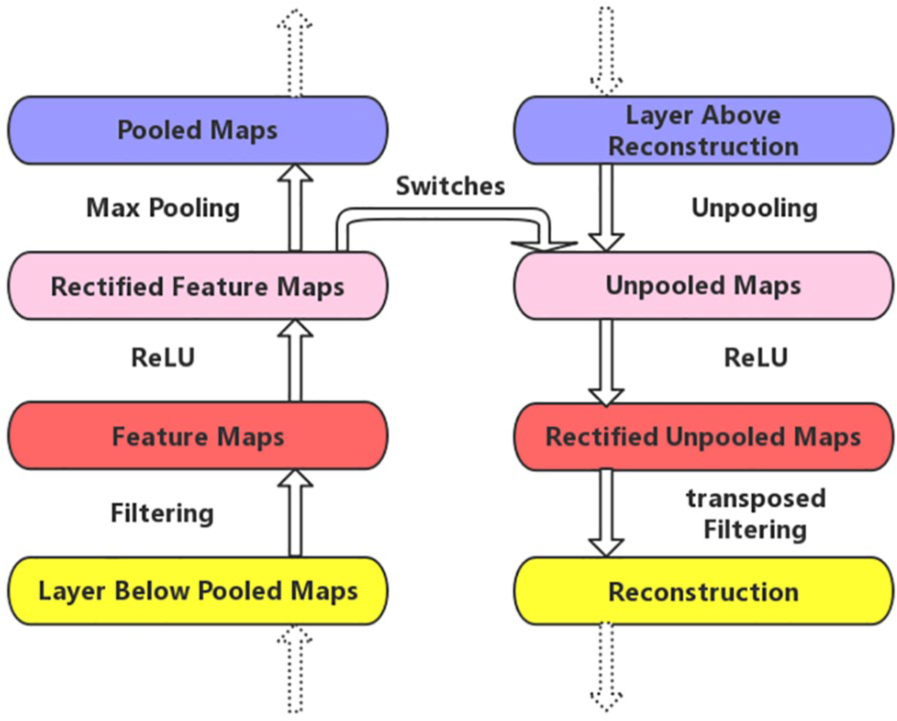
In the convolutional networks, the max-pooling operation allows the feature maps of the layer above to capture a larger receptive field than the current layer. ⁸ It is regrettable that the max-pooling operation is nonreversible. However, we can obtain an approximate version by recording the locations of the maximum value within each pooling region in a set of switches. ²⁶ Within each neighborhood of the feature maps, we can record both the value and location of the maximum value. Pooled maps store the max-values, while switches record the locations of max-values.

Unpooling

We can perform the unpooling operation when we obtain the pooled maps and switches. Projecting down from previous layers uses the pooled maps and switches generated by the max-pooling in the convolutional networks on the way up. ¹³ For the sake of holding the invariance of the activation, the unpooling operation uses these switches to array the reconstructions from the higher layers into appropriate locations in the deconvolutional networks. ²⁶ The corresponding unpooling operation is shown in Figure 2.

Figure 2.

An illustration of the switch and unpooling operation in a deconvolutional network. Using switches that record the locations of the local maximum for each pooling layer in a convolutional network. The same color represents the same position between the original feature map and the unpooled feature map.

Deconvolution

The convolutional network uses convolution kernels to convolve the feature maps from the layer above. To invert this, the deconvolutional network uses transposed versions of the same convolution kernels. To visualize a convolutional network, a deconvolutional network is attached to each of its hidden layers, as illustrated in Figure 3, providing a continuous path back to the input image pixels. To evaluate a given convolutional network activation, this article sets all other values in the same layer to zero and regards the feature maps as input to the attached deconvolutional network layers. ¹³ Then, we can successively reconstruct the activation in the layer beneath and repeat this operation until the input pixel space is reached.

Figure 3.

An illustration of a deconvolutional network layer (right) attached to a convolutional network layer (left). The same color represents the analogous space function between the convolutional network and the deconvolutional network. The deconvolutional network will reconstruct approximate features from the layer beneath.

Feature analysis

We have performed several experiments on the feature analysis of fabric images. However, there are 4224 feature maps in VGG16, and we can not show all the visualization experimental results due to the limited space. We take only one of the most representative defective images as an example to observe the feature extraction process in deep neural networks. We can analyze the deep feature from fabric defect images when the experimental environment meets the requirements (the development environment is exactly the same as that in the previous section). Figure 4 shows a visualization of fabric defect image features in a fully trained VGG16. The visualizations are reconstructed patterns from a given fabric defect feature map, rather than sampled from the model. Projecting each separately down to the input pixel space reveals the different structures that excite a given feature map, hence showing its invariance to input characteristics.

Figure 4.

Visualization of fabric defect image features in a fully trained VGG16. We did not show all the feature maps due to the limited space. Note that the experimental results were randomly sampled, and we did not deliberately select the results. A complete high-definition picture can be found at the following address: https://github.com/ZCmeteor.

The features in fabric defect images contain texture features and defect features. Our target is to distinguish the two features to detect whether the fabric is defective. The original image has a broken-end phenomenon caused by a faulty weaving process, which is one of the most common defects in fabric production. The projecting operations from each layer show the hierarchy of image features in the convolutional network.

The first layer shows the simplest edge and color features. The second layer responds to the outlines and other boundary conjunctions. In the third layer of VGG16, parts of the feature maps in the convolutional layers hold the original information from the fabric images to the maximum extent. Layer 4 shows a more pronounced change than the previous layer. Layer 5 has more complex feature information, capturing similar textures. Notably, in the picture of Row 1, Column 2 and Row 3, Column 2, there is a strong activation at the center of the feature map. This activation means that the defect features can be separated by convolutional filters, which is very helpful for defect identification in the back-end docking Softmax classifier. Layers 6 and 7 show clearer details than layer 5. There is no pooling operations between 8–10 convolutional layers. Most of the feature maps in the three layers have extracted defect features, some of which have been completely separated from the fabric features. Layers 11–13 show entire objects with significant texture variation, and the last three convolutional layers have hardly evolved. The black block is caused by the instability of gradient propagation. In other fabric feature visualization experiments, feature evolution stops at layers 8–10.

In general, a defective fabric image is covered by consecutive rectification and pooling in VGG16 to mask the texture features so that the defects can be separated. However, the visualization of convolutional layers shows that the defect features and texture features in most feature maps are not completely separated, and there is considerable redundant information in the last few layers of the convolutional network. In the next section, we will attempt to change the network structure so that it can clearly distinguish the different features from fabric defect images, and the efficiency of the defect identification system is improved by substantially reducing the number of redundant parameters.

Configuration optimization

Architecture

In this section, we attempt to change the architecture of VGG16 to speed up the operation of overall system while ensuring recognition accuracy. After a detailed visualization analysis, we found that complete features could be extracted before layer 10 in VGG16 network. Therefore, the VGG network does not require as many convolution operations as we initially configured for fabric defect detection. Ten convolutional layers containing 3 × 3 receptive field filters can meet the peak performance (as shown in Figure 5). Second, the model does not require many parameters in the fabric defect recognition task. The original VGG16 was used for the ImageNet Large-Scale Visual Recognition Challenge ²⁷ to divide the target images into 1000 classes. However, in the task of fabric defect recognition, we only need to classify the target fabric images into two categories: normal or abnormal. Therefore, the system can achieve very high recognition accuracy with only a few parameters in the fully connected layers.

Figure 5.

A network ablation experiment on VGG16 revealed that holding a compatible depth for specific recognition tasks, rather than “deeper is better,” is crucial for the system performance.

In the field of automated surface inspection, accuracy and efficiency in a discrimination system often cannot be obtained simultaneously. In some sense, these two attributes are mutually exclusive. If the number of network parameters is too small, then some fabric images with complicated texture will be difficult to recognize. If the number of parameters is too large, then the convolutional model will be very redundant, ²⁸ which is inconvenient to implement it in industrial fields. We have tried comprehensive ablation experiments and finally obtained the optimal network configuration that balances the trade-off between model volume and recognition accuracy. The ablation experiment results are showed in Figure 5, and the optimal convolutional network configurations are exhibited in Table 1.

Table 1.

The configuration of 10 convolutional layers in our model.

LZFNet configuration
Hidden layers	Layer 1	Layer 2	Layer 3	Layer 4	Layer 5	Layer 6	Layer 7	Layer 8	Layer 9	Layer 10
Padding	1	1	1	1	1	1	1	1	1	1
Filter	3 × 3	3 × 3	3 × 3	3 × 3	3 × 3	3 × 3	3 × 3	3 × 3	3 × 3	3 × 3
Stride	1	1	1	1	1	1	1	1	1	1
Channel	64	64	128	128	256	256	256	512	512	64
Rectification	ReLU	ReLU	ReLU	ReLU	ReLU	ReLU	ReLU	ReLU	ReLU	ReLU
Max-pooling	2 × 2	2 × 2	none	2 × 2	none	none	2 × 2	none	none	2 × 2

All our convolutional network layer configurations are designed using the same principles. Our model is denoted as “LZFNet”. There are 12 weight layers in it, which includes 10 convolutional layers and 2 fully connected layers. The filter kernels carry a 3 × 3 pixel window in the entire network. In the same way, the convolution stride is fixed to one, and the padding is 1 pixel for the 3 × 3 filters. All hidden layers are equipped with the ReLU ⁸ nonlinearity as before. Spatial pooling is carried out by five max-pooling layers, which are slightly different from the location of pooling layers in the original VGG model. Max-pooling is performed over a 2 × 2 receptive field with stride two.

In the fine-tuned VGG16, the convolutional layer parameters, which play a key role in feature extraction process for the target images, only account for 10.9% of the entire model parameters. However, more than 89% of the parameters are distributed in fully connected layers at the top of the model, especially the first fully connected layer. There are more than 102.7-million parameters in the first fully connected layer, and the second fully connected layer still has more than 16.7-million parameters. Therefore, many network parameters ensure the high recognition accuracy in the VGG model. However, for fabric defect detection in industrial fields, too many weights not only make the model redundant, which is laborious to implement it in a small system (e.g. field-programmable gate array and embedded system), but also increase the computational load of the defect recognition system and reduce the production efficiency in a textile enterprise. It is worth noting that after many experiments,^16,23,29,30 we found that too many redundant parameters may reduce the recognition accuracy for some fabrics with relatively simple texture. Thus, there are only two fully connected layers at the top of our model. Our configuration of the fully connected layers is similar in conventional convolutional networks; only the number of channels was reduced to 2048 and 2, respectively. The total number of fully connected layer parameters is 6.4 million in our model, which accounts for only 5.3% of the fully connected layer parameters in original VGG16 network.

Experimental comparison

In this section, we will provide a detailed performance comparison between the improved VGG16 and original model. To obtain a fairer comparison, here we use exactly the same experimental environment and database, as in the previous section. In the same way, we did not employ random initialization but used the pretrained weights as the initial value of the model and then trained it with this initialization strategy.

Training

Our model training procedure generally follows the “Fine-tuning VGG16” section. The training set we used is exactly the same as in the previous section, containing approximately 3000 normal fabric images and approximately 3000 defective fabric images. To avoid ambiguity, we choose the parameters pretrained by ImageNet as the initial values of the model in the same way, then freeze the parameters of the first seven convolutional layers and only train the last five layers. The input to our convolutional network is a fixed-size 224 × 224 RGB fabric image, and only preprocessing we do is subtracting the mean RGB value from each pixel during training. The mini-batch size was set to 64, and the momentum term was set to 0.9. The training was regularized by dropout regularization for the first fully connected layers with a rate of 0.5. We did not anneal the learning rate for the preinitialized layers, holding it to 10⁻⁴ during learning. Each input image takes 5.8 milliseconds to train, and the training was stopped after 2000 iterations. The entire training process takes 39 min. Our model training takes less time than the original model, because of a small number of parameters.

Testing

The database consists of defective images and defect-free images, which are packaged into two separate files with the folder name as the labels. This packaging is equivalent to the labels that have been attached to each image without the need to manually make the label files. To avoid the partiality in our model, we input defect images and normal images into the fully trained LZFNet to generate their own accuracy. A total of 976 defect images and 24 normal images were identified in the dataset containing 1000 defective fabric images, and the TNR was 97.6%. A total of 986 normal images and 14 defect images were identified in the dataset containing 1000 normal fabric images, and the TPR was 98.6%. Overall, the total correct recognition rate of the whole system is 98.1%, and it takes 13.8 milliseconds on average for each input image to be recognized. The performance comparison with the original VGG16 is exhibited in Table 2. The “model size” means the disk space occupied by “.data” files. The “MAdds” represent the number of multiply-add combined operation.

Table 2.

The performance indexes for our model against VGG16.

Performance comparison
Model	TNR	TPR	Accuracy	Parameters number	Model size	MAdds
VGG16	97.3	98.1	97.7	134 M	537 MB	15470M
LZFNet	97.6	98.6	98.1	12M	51MB	351M

TNR: True Negative Rate; TPR: True Positive Rate; VGG: Visual Geometry Group.

The fabric image database that we used contains a limited number of fabric images, and better experimental results will be obtained if more fabric images can be provided for model training. At present, our team is actively cooperating with several textile enterprises to build a dataset consisted of over hundred thousand labeled high-resolution fabric images, to further improve performance of the recognition system in terms of the data.

Conclusion

First, this article analyzed the shortcomings of the traditional convolutional networks for fabric defect detection, and proposed a special VGG16 that can be applied to detect defects in fabrics that have complicated textures, to solve the problem that complicated texture fabrics cannot be effectively detected at present. To optimize the VGG convolutional network, a deconvolutional network was attached to each of its layers and provided a continuous path back to the image pixel space. Using this visualization technique, we then visualized the whole feature extraction process in the VGG16 network and attempted to change the architecture of VGG16 to speed up the overall system operation while maintaining the recognition accuracy and to be more efficient to implement it in a small system. Finally, after a series of improvements, a new convolutional neural network was acquired that exhibited better recognition performance for the fabric images. The total number of parameters is only 12 million in our model, which is specifically tailored for fabric defect recognition in textile factories.