Sage Journals: Discover world-class research

Abstract

In this article, a method based on gray projection is proposed for automatic measurement of surface braiding angle and pitch length of braided composite preforms. The surface braiding angles are measured by rotated gray projection. First, the original image is preprocessed using Lab transform and block-matching and three-dimensional filter. Then, edge map of gray scale is acquired based on phase congruency and non-maximum suppression. Third, edge direction angles are computed by image rotation and gray projection. Finally, the average surface braiding angles are measured from the edge direction angles. The pitch lengths are measured by cropped gray projection. First, the original image is filtered by an artistic edge and corner enhancing filter. Second, block images are cropped based on gray projection. Finally, pitch lengths are measured by block images gray projection. Experimental results show that the proposed method can achieve the automatic measurement of average surface braiding angle and average pitch length of two-dimensional braided composite preform with high accuracy.

Keywords

Braided composite preform surface braiding angle pitch length gray projection

Introduction

As representatives of lightweight materials with high stiffness and strength, fiber-braided composite materials have been widely used in fields of aerospace, automotive, military, energy, sports, and so on.^1,2 The braid pattern evolves from an interaction of the yarn movement, which is interlacing three or more threads diagonally to the product axis in order to obtain a thicker, wider, or stronger product or to cover some profile,^3,4 forming braided preforms, then the preforms are consolidated by resin transfer molding (RTM)⁵ or vacuum assisted resin transfer molding (VARTM),^6,7 as composites.

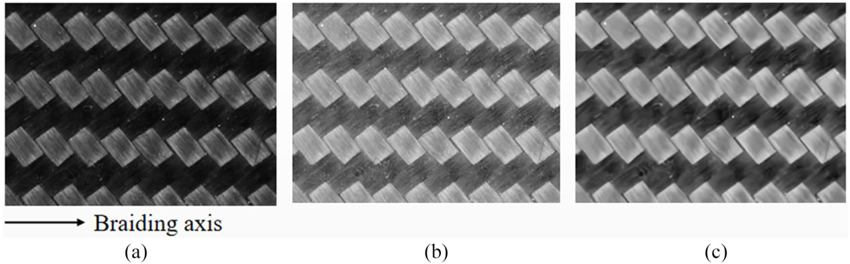
Generally, the braided structures include three-dimensional (3D) braid (see Figure 1(a)) and two-dimensional (2D) braid (see Figure 1(b) to (c)) according to how the yarns interlace into 3D space or 2D plane.⁸ The 2D braided structures can be classified as biaxial braid (see Figure 1(b)) and triaxial braid (see Figure 1(c)) according to whether there are axial yarns or not.⁹ Biaxial braids is very basic and most common form of 2D braids, which are composed of interlacing yarns arranged in two directions.¹⁰ According to the braiding patterns, biaxial braids are classified as diamond, regular, and Hercules¹¹ (see Figure 2).

Figure 1.

Structures of 3D and 2D braids: (a) 3D, five directional braid; (b) 2D biaxial regular braid; and (c) 2D triaxial braid.

Figure 2.

Structures of 2D braids: (a) diamond braid, (b) regular braid, and (c) Hercules braid.

The surface braiding angle θ is defined as the angle between the longitudinal direction of the braided preform and the deposited fibers,¹² and pitch length h is the preform take-up length for one machine cycle,^13,14 as shown in Figure 3. Surface braiding angle and pitch length are two important parameters to affect the kinematic analysis of the process, geometry of braided composite.^9,14 For example, the surface braiding angle θ can be calculated by Heieck et al.,⁹ Potluri et al.¹⁵

θ = \tan^{- 1} (\frac{ω R}{v})

(1)

where R is the radius of cylindrical mandrel (cm), v is take-up speed (cm/s), and ω is the average angular velocity of bobbins around the machine center (rad/s). Sun and Sun¹⁶ indicated that braiding angle went down with increased pitch length. The surface braiding angle and pitch length are also important parameter of influencing the mechanical behavior of braided composite,^15,17–20 for instance, as the surface braiding angle increase, the mismatch between longitudinal and transverse stiffness become less pronounced, with a tendency toward balanced Poisson’s ratios for the [0°/± 60°] material.²¹ Zou et al.²² indicated that the radial force is higher with shorter pitch length when surface braiding angle is fixed.

Figure 3.

Surface braiding angle and pitch length: (a) in an ideal scenario and (b) in a practical scenario.

In industrial, manual measurement of average surface braiding angle is still the main method, which is time- and manpower-consuming.

At present, several automatic measurement methods^23,24 have been proposed for 3D braided composites preforms. For the parameter measurement of 2D braided preforms, Hunt and Carey²⁵ applied a frequency domain method to achieve automatic real-time of 2D braided preform. This method is more suitable for the fabric images with high contrast between fiber bundle and background and is easy to be affected by the contrast of braided axis. Few methods are proposed for pitch length measurement of 2D braided composite preform. Thus, it is significant to achieve the automatic measurement of the two parameters. In this article, we propose a new automatic method based on gray projection to measure surface braiding angle and pitch length of 2D biaxial regular braided composite preforms.

Materials and experimental methods

Materials

The tested 2D biaxial regular braided tubes were supplied by Shuomin Technology Co. Ltd, China. The braided fibers include carbon, glass, and aramid fiber, and the average diameters of the fiber filaments are, respectively, 5.70, 7.91, and 11.02 µm, tested by the School of Textiles of Tianjin Polytechnic University using the fiber fineness analyzer manufactured by Laizhou Electron Instrument Co., Ltd. (Taiyuan, China). Since the braided tubes are easy to stretch, they are pasted on horizontal plates using double-sided tapes. And the double-sided tapes pasted on the back of the fabrics cover all the areas of the fabrics to make sure that the fiber tows of the fabrics can be well fixed on the plane, as illustrated in Figure 4 (acquired by Redmi 4X mobile phone).

Figure 4.

Fabric sample: (a) glass-fiber fabric, (b) aramid-fiber fabric, and (c) carbon-fiber fabric.

Image acquisition

The original images are acquired using the image acquisition system shown in Figure 5. First, the CCD camera (Vieworks VA-8MC-M16AO; 3296 × 2472 pixels; Area CCD camera) with camera lens (Nikkor 28mm f/2.8D) and circular polarizing filter (CPF) (NiSiCPL52mm) attached is vertically installed above the fabric, and the micrometer is put on one side of the fabric for calibration, keeping the surfaces of the micrometer and the fabric on the same horizontal plane. Then the dome light source (DLS) (OPT-RID180-RGB) is put in front of the fabric, making the camera’s optical center go through the central axis of the DLS light hole and also the center of the fabric surface. Finally, the camera exposure value and focal length, and the rotated angle of CPF are adjusted, and a clear image is selected.

Figure 5.

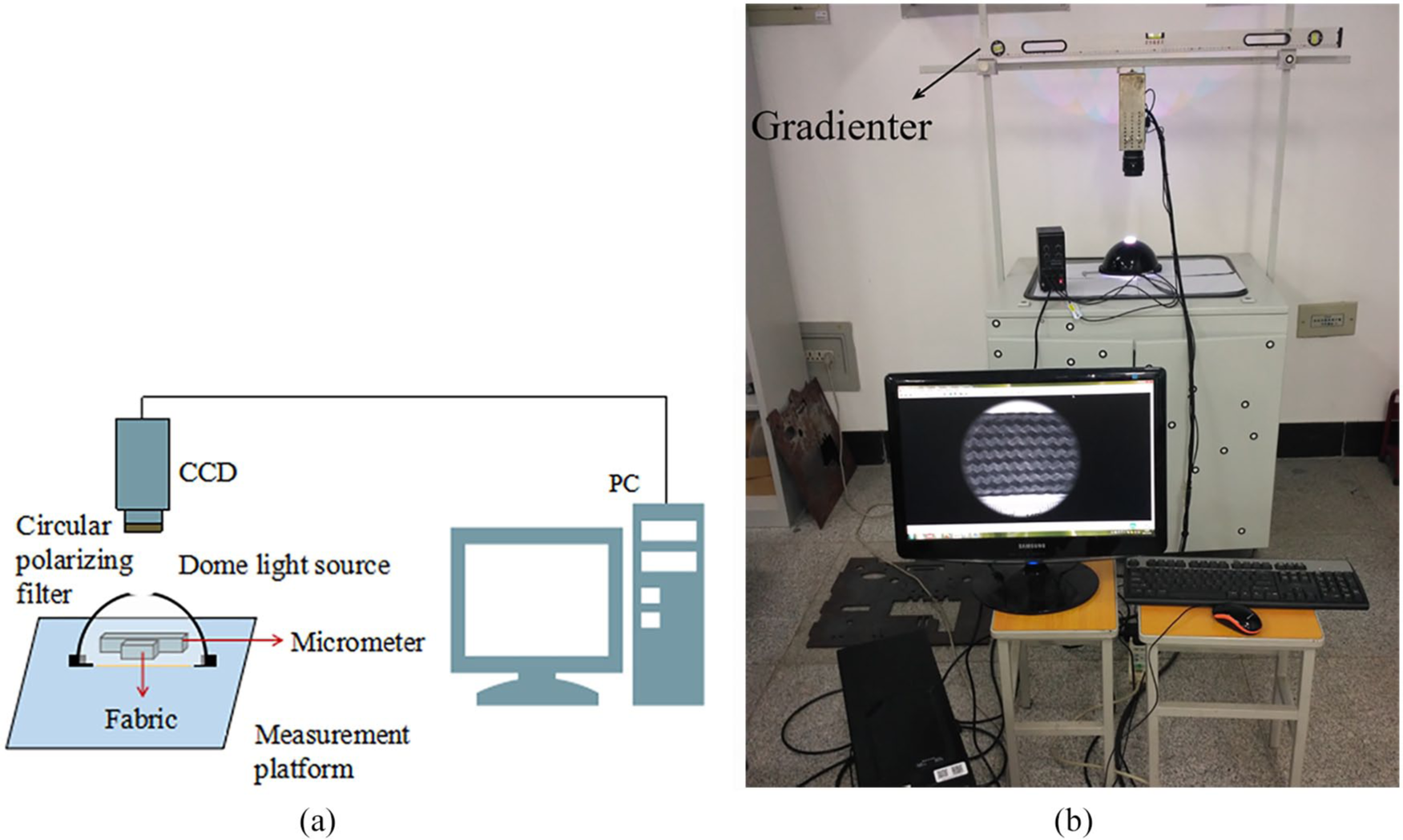
Image acquisition system: (a) system diagram and (b) physical system.

During the image acquisition, to make sure that the CCD camera is vertically installed above the fabric, the gradienter is stuck to the shelf by its own magnet (see Figure 5(b)), then it is adjusted to be horizontal according to the gradienter reading. To test the accuracy of the acquired images, we compare the image corrected by calibration board (GQ-H56–3.5; expansion coefficient: α = 8.6 × 10⁻⁶/°C) (see Figure 6) and HALCON software.²⁶ The process of distortion correction is described as follows: first, obtain the distortion parameters of the camera by finding the marked points centers of the calibration board images (see Figure 7); then correct the image based on the distortion parameters.

Figure 6.

The 7 × 7 HALCON calibration board.

Figure 7.

Calibration board images: (a) I₁, (b) I₂, (c) I₃, (d) I₄, (e) I₅, (f) I₆, (g) I₇, (h) I₈, (i) I₉, (j) I₁₀, (k) I₁₁, (l) I₁₂, (m) I₁₃, (n) I₁₄, (o) I₁₅, (p) I₁₆, (q) I₁₇, (r) I₁₈, (s) I₁₉, (t) I₂₀, (u) I₂₁, (v) I₂₂, (w) I₂₃, (x) I₂₄, (y) I₂₅, and (z) I_26.

Figure 8 is image before and after distortion correction. It can be seen that there is almost no difference between the image before and after distortion correction. So the images acquired by the system have high accuracy.

Figure 8.

Before and after correlation: (a) before correlation, (b) after correlation, (c) local amplification of (a), and (d) local amplification of (b).

Figure 9 is the images acquired based on “CCD camera + nature light source” and based on the proposed system. It can be seen that images acquired based on “CCD camera + nature light source” have reflections with varying degrees (see Figure 9(a), (c), and (e)), and the surface reflections on Figure 9(b), (d), and (f) have been weakened efficiently, and also the images (especially carbon-fiber fabrics) have higher contrast in texture structure. The reasons are described as follows: first, the DLS can make the light uniformly illuminate on the fabric surface; second, the CPF has the characteristic of filtering reflection in a certain direction.^27,28

Figure 9.

Images acquired by common acquisition system and by our system: (a) carbon-fiber fabric acquired by “CCD camera + nature light source,” (b) carbon-fiber fabric acquired by our acquisition system, (c) glass-fiber fabric acquired by “CCD camera + nature light source,” (d) glass-fiber fabric acquired by our acquisition system, (e) aramid-fiber fabric acquired by “CCD camera + nature light source,” and (f) aramid-fiber fabric acquired by our acquisition system.

Surface braiding angle measurement

Before surface braiding angle measurement, the original acquired image F_ori is first preprocessed by Lab transform²⁹ and block-matching and 3D filter (BM3D)³⁰ to enhance contrast and filter noise, respectively.

The CIE-Lab color space introduced by the Commission Internationale de L’Eclairage (CIE) in 1976 has three axes: L, a, and b. It first converts from R, G, and B space into X, Y, and Z space, then converts X, Y, and Z into L, a, and b space, using equations (2) to (4) as follows²⁹

(\begin{array}{l} X \\ Y \\ Z \end{array}) = [\begin{array}{l} 0.412453 0.357580 0.180423 \\ 0.212671 0.715160 0.072169 \\ 0.019334 0.119193 0.950227 \end{array}] (\begin{array}{l} R \\ G \\ B \end{array})

(2)

{\begin{cases} L = 116 f (Y) - 16 \\ a = 500 [f (\frac{X}{0.9504}) - f (Y)] \\ b = 200 [f (Y) - f (\frac{Z}{1.0887})] \end{cases}

(3)

f (x) = {\begin{cases} x^{\frac{1}{3}}, x > {(\frac{6}{29})}^{3} \\ \frac{1}{3} {(\frac{29}{6})}^{2} x + \frac{4}{29}, x \leq {(\frac{6}{29})}^{3} \end{cases}

(4)

We use L-channel image F_L to achieve image enhancement. Then the L-channel image F_L is filtered by BM3D.

BM3D achieves image filter in 3D transform domain by combining sliding-window transform processing with block-matching. First, divide the image into small blocks and choose one block as currently processed one, then search blocks which are similar to the currently processed one. Second, stack the matched blocks together, forming a 3D array, which have high level of correlation. Third, exploit this correlation by applying a 3D decorrelating unitary transform and attenuate the noise by shrinkage of the transform coefficients, and subsequent inverse 3D transform yields estimates of all matched blocks. Finally, repeat this procedure for all image blocks in sliding manner, and compute the final estimate as weighed average of all overlapping block-estimates.

Figure 10 is the process of image preprocessing, where Figure 10(a) is original image acquired by image acquisition system, and Figure 10(b) and (c) are the L-channel image and BM3D filtered image, respectively. It can be seen that original image preprocessed by Lab transform and BM3D filter has higher contrast and weaker fiber texture.

Figure 10.

Original image and the preprocessing image: (a) original image F_ori, (b) L-channel image F_L, and (c) BM3D filtered image F_BM3D.

After preprocessing, image F_BM3D is then processed for average surface braiding angle measurement based on rotated gray projection. The detailed steps are described as follows:

Step 1. Calculate phase congruency maps³¹ of images F_BM3D (see Figure 11(a)), getting images F_PC (see Figure 11(b)).

Step 2. Calculate non-maximum suppression maps³² of F_PC, getting images F_nom (see Figure 11(c)).

Figure 11.

Process of edge direction angles detection: (a) F_BM3D, (b) F_PC, (c) F_nom, (d) rotated F_nom at −36.1°, (e) gray projection curve of (d), (f) rotated F_nom at 48.8°, and (g) gray projection curve of (f).

From Figure 11(c), it can be seen that the image edges can be classified into two directions, labeled by blue ribbon arrow lines. So the average surface braiding angle θ_aBM3D can be calculated by the angles θ_r+ and θ_r– between the edges of two directions and the horizontal direction (braiding axis direction)

θ_{a B M 3 D} = \frac{(θ_{r +} + | θ_{r -} |)}{2}

(5)

And the angles θ_r+ and θ_r– can be calculated based on image rotation, described in the following steps.

Step 3. Calculate edge direction angles θ_r+ and θ_r– of image F_nom based on the principle that maximum peak value of gray projection is largest when the edge direction is perpendicular to the projection plane.

Step 3.1. Rotate image F_nom from −89° to 89° with step length 0.1 (the precision of angle can be accurate to 0.1°), getting rotated images F_roti (i = 1, 2, . . ., 1781). As shown in Figure 11(d), where the rx–ry are coordinate axes of image rotation, and o located in the center of the image is origin of coordinate zero.

Step 3.2. Calculate gray projection images of F_roti projected on the projection plane γ (see Figure 11(d)) that is perpendicular to the image plane, getting image F_gpi.

Step 3.3. Compute the maximum peak values P_i in each F_gpi. Then obtain the angle corresponding to the maximum value P_max+ of P_i when the rotated angles are positive, as θ_r+, and the angle corresponding to the maximum value P_max– of P_i when the rotated angles are negative, as θ_r–.

As shown in Figure 11(d) to (g), for example, in Figure 11(d) and (e), P_max– = 24.44, θ_r– = –36.1°, and the edge direction of direction 1 is perpendicular to the projection plane γ, and in Figure 11(f) and (g), P_max+ = 25.28, θ_r+ = 48.8°, and the edge direction of direction 2 is perpendicular to the projection plane γ.

Step 4. Compute average surface braiding angle.

The average surface braiding angle of image F_BM3D is calculated by equations (5).

As shown in Figure 11(d) to (g), the average surface braiding angle θ_aBM3D = (48.8 + 36.1)/2 = 42.45°.

Step 5. Crop block images F_Cek, F_Rdk, F_Ldk, F_Ruk, and F_Luk (k = 1, 2) from image F_BM3D, where the subscripts Ce, Rd, Ld, Ru, and Lu for F are used to indicate the block images cropped by starting from center, right down, left down, right up, and left up of F_BM3D. F_Cek, F_Rdk, F_Ldk, F_Ruk, and F_Luk can be calculated by equations (6) to (10)

F_{C e k} = F_{B M 3 D} (\begin{array}{l} \frac{m}{6} - (k - 1) \frac{m}{12} : \frac{5 m}{6} + (k - 1) \frac{m}{12}, \\ \frac{n}{6} - (k - 1) \frac{n}{12} : \frac{5 n}{6} + (k - 1) \frac{n}{12} \end{array})

(6)

F_{R d k} = F_{B M 3 D} (\frac{m}{3} - (k - 1) \frac{m}{6} : m, \frac{n}{3} - (k - 1) \frac{n}{6} : n)

(7)

F_{L d k} = F_{B M 3 D} (\frac{m}{3} - (k - 1) \frac{m}{6} : m, 1 : \frac{2 n}{3} + (k - 1) \frac{n}{6})

(8)

F_{R u k} = F_{B M 3 D} (1 : \frac{2 m}{3} + (k - 1) \frac{m}{6}, \frac{n}{3} - (k - 1) \frac{n}{6} : n)

(9)

F_{L u k} = F_{B M 3 D} (1 : \frac{2 m}{3} + (k - 1) \frac{m}{6}, 1 : \frac{2 n}{3} + (k - 1) \frac{n}{6})

(10)

where m and n are, respectively, the row number and column number of image F_BM3D. As shown in Figure 12, for intuitive show, the cropped images are superimposed on the original images, from small to large.

Figure 12.

Cropped block images: (a) F_Cek, (b) F_Rdk, (c) F_Ldk, (d) F_Ruk, and (e) F_Luk.

Step 6. Repeat step 1–4 to detect the average surface braiding angles θaCek, θ_aRdk, θ_aLdk, θ_aRuk, and θ_aLuk of block images F_Cek, F_Rdk, F_Ldk, F_Ruk, and F_Luk (k = 1, 2), respectively, and use the average value θ_a as the final average surface braiding angle, as computed by

θ_{a} = \frac{(\begin{array}{l} θ_{a B M 3 D} + \sum_{k}^{2} θ_{a C e k} + \sum_{k}^{2} θ_{a R d k} + \sum_{k}^{2} θ_{a L d k} \\ + \sum_{k}^{2} θ_{a R u k} + \sum_{k}^{2} θ_{a L u k} \end{array})}{11}

(11)

Pitch length measurement

Before pitch length measurement, the original acquired image F_ori is first preprocessed by an artistic edge and corner enhancing filter (AECE)³³ to filter the effects of fiber texture and noise.

AECE is a noniterative edge and corner preserving smoother. As shown in Figure 13, the original image F_ori (see Figure 13(a)) filtered by AECE has less noise and fiber texture (see Figure 13(b)), which is better for the flowing image processing.

Figure 13.

Original image and filtered image: (a) original image F_ori and (b) AECE filtered image F_ae.

Then the AECE filtered image F_ae is processed for average pitch length measurement based on cropped gray projection. The detailed steps are described as follows:

Step 1. Project image F_ae on plane γ, getting gray projection curve F_po. As shown in Figure 14(a), where the plane γ is perpendicular to image F_ae, then smooth F_po, getting F_p (see Figure 14(b)).

Step 2. Crop block images from F_ae based on projection image F_p. First, in F_p, calculate the locations d_pti (i = 1, 2, . . .) of peak and trough. Then cut image F_ae by using d_pti as the row border, getting block images F_bi (see Figure 14(c)).

Step 3. Project block images F_bi to the plane β, getting projection curves, and smooth these curves, getting F_bpk (k = 1, 2, . . .). The plane β is shown in Figure 14(a) and is perpendicular to block images F_bi. Then, calculate the peak-to-peak values and trough-to-trough values in F_bpk (k = 1, 2, . . .), getting d_plpj (j = 1, 2, . . .). Then obtain the average values ${\bar{d}}_{a p l p}$ of d_plpj, which is the pixel distance of average pitch length.

Figure 14.

Process of average pitch length measurement: (a) image F_ae and projection planes, (b) F_p, (c) block images F_bi, and (d) F_bp₁.

Figure 14(d) is projection image of one block image F_b₁, for example.

The principle of this step is described as follows: first, in Figure 14(c), the clock image F_b₁, for example, the distance between A_i and A_j (labeled by yellow points) or distance between B_i and B_j (j = i + 1) (labeled by blue points) (i = 1, 2, 3, . . .), is equal to the pitch length in pixels. Second, as shown in Figure 14(d), for example, the peak and trough values of F_bp₁ approximately reflect points A_i and B_i of F_b₁ (see Figure 14(c)), respectively. Thus, the single pitch length in pixels can be obtained by calculating the peak-to-peak values and trough-to-trough values of projection image F_bp₁. Similarly, single pitch lengths in pixels in other block images can be calculated, and the average pitch length in pixels can be obtained based on all the single pitch lengths.

Step 4. Calculate average pitch length by

d_{a p l} = {\bar{d}}_{a p l p} \times d_{c}

(12)

where d_c defined as calibration value represents the actual distance per pixel.

Results and discussion

In this section, five types of images are tested using the proposed method, and each type contains 35 images, as shown in Figure 15, where Figure 15(a) to (e) are, respectively, glass-fiber, aramid-fiber, carbon (6k), carbon-fiber (3k), and carbon-fiber (3k) 2D biaxial regular braided images.

Figure 15.

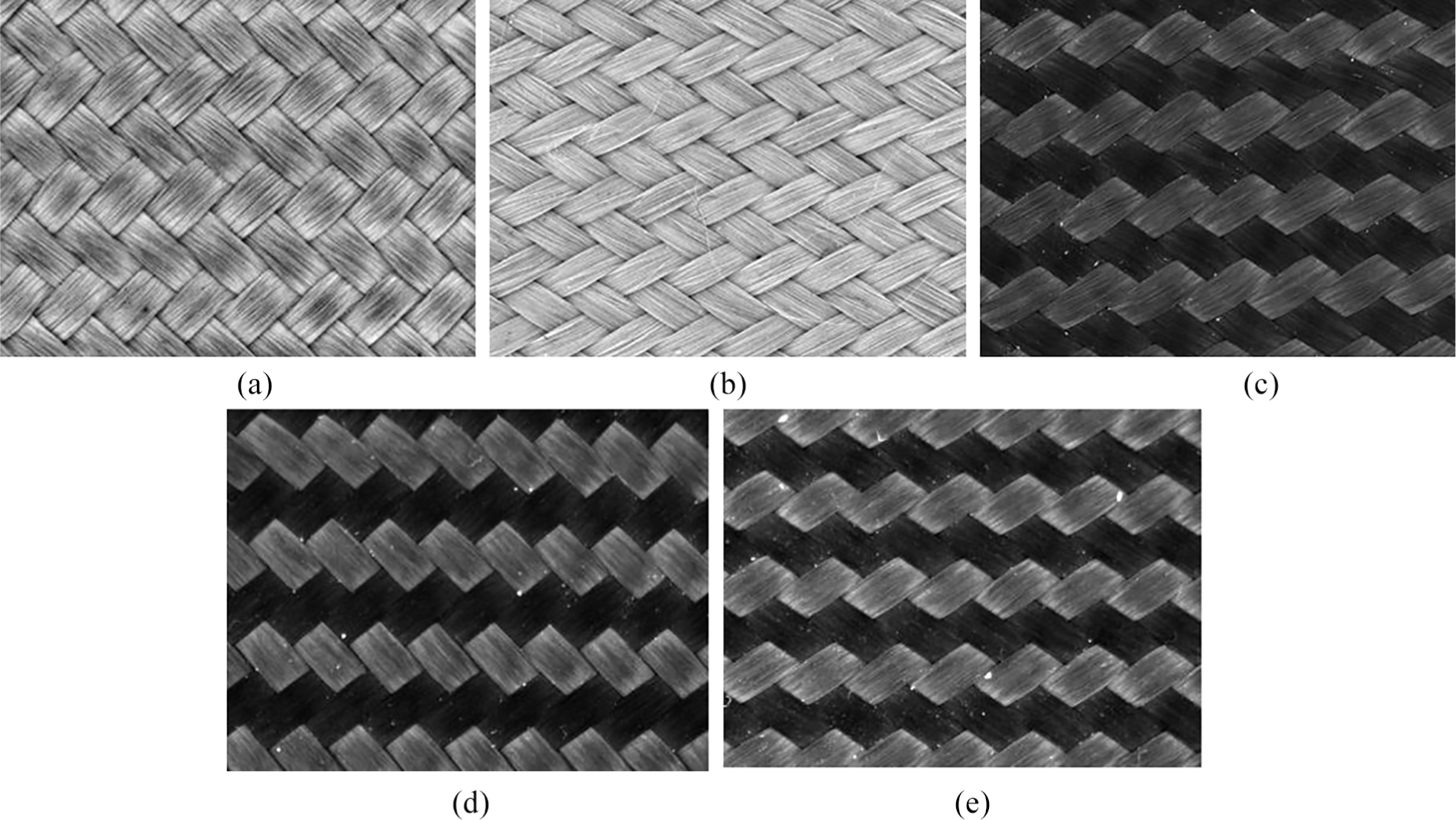
Sample images: (a) F₁ (glass-fiber), (b) F₂ (aramid-fiber), (c) F₃ (carber fiber (6k)), (d) F₄ (carber fiber (3k)), and (e) F₅ (carber fiber (3k)).

Manual measurements of average surface braiding angle and pitch length are used to benchmark our proposed method. Manual measurements of average surface braiding angle is based on electronic protractor, as demonstrated in Figure 16(a), for example, one angle θ is measured to be 62.85°, and thus the single surface braiding angle θ_M is set to θ_M = θ/2 = 62.85/2≈31.43°. The average surface braiding angle θ_aM is the average value of all single surface braiding angles, calculated by

θ_{a M} = \frac{(\sum_{i = 1}^{n} \frac{θ_{i}}{2})}{n}

(13)

where n is the number of single surface braiding angles measured. Figure 16(b) is the labeled single angles θ_i (i = 1, 2, 3, . . ., 35) to be measured, and here n = 35. The manual measurement of pitch length is based on clicking corner points of fabric image on computer screen, as displayed in Figure 16(c), for example, the coordinates of clicked points are A(97, 192) and B(99, 248), respectively. So one pitch length is calculated as d_plAB = d_c × d_AB, where d_c is calibration value, that is, the true distance per pixel, and $d_{A B} = \sqrt{{(99 - 97)}^{2} + {(248 - 192)}^{2}}$ is distance between points A and B. The average pitch length d_aM can be calculated by

d_{a M} = \frac{(\sum_{i = 1}^{k} d_{p l i})}{k}

(14)

where k is the number of single pitch lengths measured. Figure 16(d) is the labeled corner points to be measured, here we only labeled the first two lines’ corners, for example, pitch lengths d_plAiAj (i = 1, 2, 3, . . .; j = i + 1) can be calculated as d_plAiAj = d_c × d_AiAj, where d_AiAj is distance between corners A_i and A_j. Similarly, pitch lengths d_plBiBj and pitch lengths in other lines can be defined and calculated. So the average pitch length of Figure 16(d) can be computed by equation (14).

Figure 16.

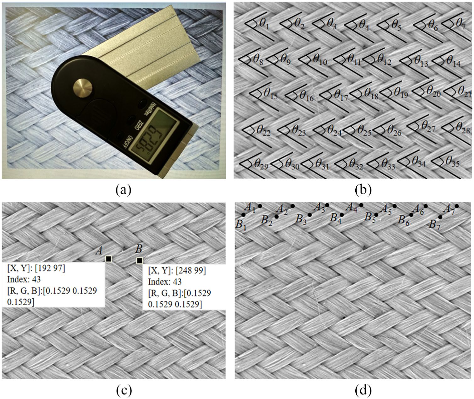
Manual measurement of surface parameters: (a) manual measurement of surface braiding angles, (b) labeled angles, (c) manual measurement of pitch lengths, and (d) labeled corners.

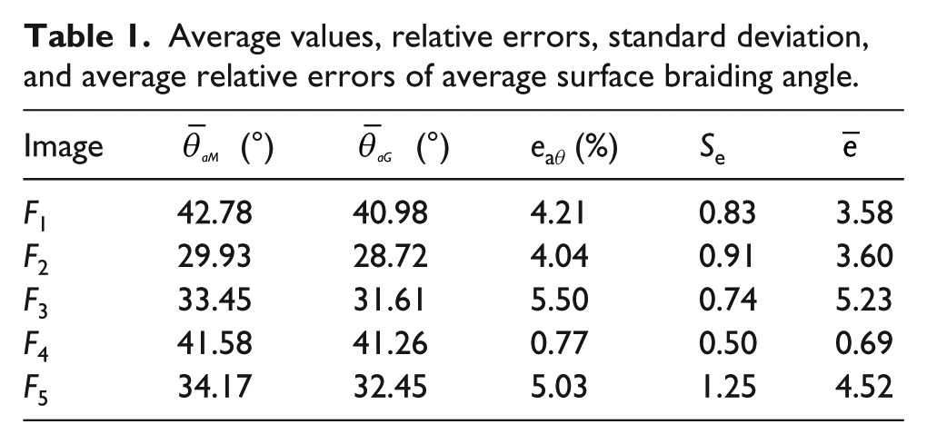
The errors of the average surface braiding angle and pitch length measured by our method relative to the manual measurements are illustrated in Figure 17, where the errors are sorted in ascending order. Tables 1 and 2 show the average values, relative errors, standard deviations, and average relative errors of average surface braiding angle and pitch length, respectively, where $\bar{θ}$ and $\bar{d}$ indicate the average values of surface braiding angle and pitch length, respectively. The subscripts aM and aG indicate the average values measured by manual and by our method, respectively. e_aθ is the errors of ${\bar{θ}}_{a G}$ relative to ${\bar{θ}}_{a M}$ , and e_ad is the errors of ${\bar{d}}_{a G}$ relative to ${\bar{d}}_{a M}$ . S_e is standard deviation of 80% relative errors, and $\bar{e}$ is average values of 80% relative errors. e_aθ, e_ad, and S_e can be calculated by

e_{a θ} = \frac{| {\bar{θ}}_{a G} - {\bar{θ}}_{a M} |}{{\bar{θ}}_{a M}} \times 100 %

(15)

e_{a d} = \frac{| {\bar{d}}_{a G} - {\bar{d}}_{a M} |}{{\bar{d}}_{a M}} \times 100 %

(16)

S_{e} = \sqrt{\frac{1}{N - 1} \sum_{i = 1}^{N} {(e_{i} - \bar{e})}^{2}}

(17)

where in equations (17), N = 35, e_i is each error of average surface braided angles (or average pitch lengths) measured by our method relative to manual measurement, and $\bar{e}$ is average value of relative errors.

Table 1.

Average values, relative errors, standard deviation, and average relative errors of average surface braiding angle.

Image	${\bar{θ}}_{a M}$ (°)	${\bar{θ}}_{a G}$ (°)	e_aθ (%)	S_e	$\bar{e}$
F ₁	42.78	40.98	4.21	0.83	3.58
F ₂	29.93	28.72	4.04	0.91	3.60
F ₃	33.45	31.61	5.50	0.74	5.23
F ₄	41.58	41.26	0.77	0.50	0.69
F ₅	34.17	32.45	5.03	1.25	4.52

Table 2.

Average values, relative errors, standard deviation, and average relative errors of average pitch length.

Image	${\bar{d}}_{a M}$ (°)	${\bar{d}}_{a G}$ (°)	e_ad (%)	S_e	$\bar{e}$
F ₁	2.54	2.54	0	0.52	0.93
F ₂	2.76	2.83	2.54	1.60	2.47
F ₃	4.21	4.19	0.48	0.18	0.35
F ₄	1.87	1.89	1.07	0.35	0.87
F ₅	1.98	1.98	0	0.093	0.17

Figure 17.

Relative error curves of average surface braiding angles and pitch lengths: (a) average surface braiding angle relative errors of image F₁; (b) average pitch length relative errors of image F₁; (c) average surface braiding angle relative errors of image F₂; (d) average pitch length relative errors of image F₂; (e) average surface braiding angle relative errors of image F₃; (f) average pitch length relative errors of image F₃; (g) average surface braiding angle relative errors of image F₄; (h) average pitch length relative errors of image F₄; (i) average surface braiding angle relative errors of image F₅; and (j) average pitch length relative errors of image F₅.

The following observations are made from Figure 17, Table 1, and Table 2:

Standard deviations of relative errors, and average values of relative errors of average surface braiding angle and pitch length are small, which shows that the stability and accuracy of the results measured by our method.

In the measurement of average surface braiding angle, sample image F₄ has smaller relative errors and standard deviation than other samples, for the edges in sample F₄ are more closed to straight line than other types of samples, which has smaller impact in gray projection.

The relative errors of average pitch length are smaller than the values of surface braiding angles, for the average pitch lengths are measured based on local features of fabric image while average surface braiding angles are measured based on the overall features of fabric image.

Conclusion

This article presented a new method for automatically measuring the average surface braiding angles and pitch lengths for biaxial regular braided glass-, aramid- and carbon-fiber preforms. Some conclusions are drawn as follows:

The proposed method can not only measure surface braiding angles but also measure pitch lengths.

The phase congruency used in initial edge detection improves the accuracy of edge detection, so as to improve the accuracy of average surface braiding angle measurement.

In the calculation of average surface braiding angle, the measurement results depend on the average surface braiding angles of multiple block images, which is helpful to reduce the errors of measuring only one image.

The cropping method based on overall image projection well crop image into block images according image structure texture, which is helpful to extract local pitch length of fabric.

The proposed automatic method can be used as a foundation of computer parameter measurement for 2D braided texture analysis.

Footnotes

Declaration of conflicting interests

The author(s) declared no potential conflicts of interest with respect to the research, authorship, and/or publication of this article.

Funding

The author(s) disclosed receipt of the following financial support for the research, authorship, and/or publication of this article: This work was supported by Applied Basic Research Programs of China National Textile and Apparel Council (No. J201509) and the Program for Innovative Research Team in University of Tianjin (No. TD13-5034).

ORCID iD

Zhitao Xiao

References

Sturm

Heieck

Energy absorption capacity of braided frames under bending loads. Composit Struct 2015; 134: 957–965.

Shan

, et al. A mixed-form solution to the macroscopic elastic properties of 2D triaxially braided composites based on a concentric cylinder model and the rule of mixture. Composit Pt B Eng 2019; 156: 355–367.

Kessels

Akkerman

Prediction of the yarn trajectories on complex braided preforms. Composit Pt A Appl Sci Manuf 2002; 33(8): 1073–1081.

Kyosev

Braiding technology for textiles: principles, design and processes. Amsterdam: Elsevier, 2014.

Gao

Song

Qiu

, et al. The preparation and properties of novel structural damping composites reinforced by nitrile rubber coated 3-D braided carbon fibers. Polym Composit 2019; 40(S1): E599–E608.

Yun

Carella

Simacek

, et al. Stochastic modeling of through the thickness permeability variation in a fabric and its effect on void formation during vacuum assisted resin transfer molding. Composit Sci Technol 2017; 149: 100–107.

Abusrea

Han

Arakawa

, et al. Bending strength of CFRP laminated adhesive joints fabricated by vacuum-assisted resin transfer molding. Composit Pt B Eng 2019; 156: 8–16.

Sun

Impact shear damage characterizations of 3D braided composite with X-ray micro-computed tomography and numerical methodologies. Composit Struct 2017; 176: 43–54.

Heieck

Hermann

Middendorf

, et al. Influence of the cover factor of 2D biaxial and triaxial braided carbon composites on their in-plane mechanical properties. Composit Struct 2017; 163: 114–122.

10.

Zhao

Huang

Chen

, et al. Progressive failure prediction of a landing gear structure of braided composites. Composit Struct 2017; 161: 407–418.

11.

Kim

Ong

, et al. Prediction of material properties of biaxial and triaxial braided textile composites. J Composit Mater 2012; 46(18): 2255–2270.

12.

Boris

Xavier

Damien

The tensile behaviour of biaxial and triaxial braided fabrics. J Indus Text 2018; 47(8): 2184–2204.

13.

Tang

Postle

Mechanics of three-dimensional braided structures for composite materials-part I: fabric structure and fibre volume fraction. Composit Struct 2000; 49(4): 451–459.

14.

Byun

JH.

The analytical characterization of 2-D braided textile composites. Composit Sci Technol 2000; 60(5): 705–716.

15.

Potluri

Rawal

Rivaldi

, et al. Geometrical modelling and control of a triaxial braiding machine for producing 3D preforms. Composit Pt A Appl Sci Manuf 2003; 34(6): 481–492.

16.

Sun

Mechanical properties of three-dimensional braided composites. Composit Struct 2004; 65(3–4): 485–492.

17.

Ayranci

Carey

2D braided composites: a review for stiffness critical applications. Composit Struct 2008; 85(1): 43–58.

18.

Ayranci

Carey

Predicting the longitudinal elastic modulus of braided tubular composites using a curved unit-cell geometry. Composit Pt B Eng 2010; 41(3): 229–235.

19.

Guan

Jia

, et al. Effective elastic properties and stress distribution of 2D biaxial nonorthogonally braided composites. J Composit Mater 2012; 46(8): 997–1008.

20.

Kier

Salvi

Theis

, et al. Estimating mechanical properties of 2D triaxially braided textile composites based on microstructure properties. Composit Pt B Eng 2015; 68: 288–299.

21.

Wehrkamp-Richter

Hinterhölzl

Pinho

ST.

Damage and failure of triaxial braided composites under multi-axial stress States. Composit Sci Technol 2017; 150: 32–44.

22.

Zou

Xue

Lin

, et al. Mechanical characteristics of novel polyester/NiTi wires braided composite stent for the medical application. Result Phys 2016; 6: 440–446.

23.

Wan

Shen

Wang

Measure and research on braided angle of composites preform. J Text Res 2004; 25(3): 42–44 (In Chinese).

24.

Wan

Braided angle measurement technique for three-dimensional braided composite material preform using mathematical morphology and image texture. AUTEX Res J 2006; 6(1): 30–56.

25.

Hunt

Carey

JP.

A machine vision system for the braid angle measurement of tubular braided structures. Text Res J 2019; 89(14): 2919–2937.

26.

Qian

Wang

Study of single camera calibration based on HALCON software. J Shijiazh Tied Univ 2018; 31(3): 79–84 (In Chinese).

27.

Umeyama

Godin

Separation of diffuse and specular components of surface reflection by use of polarization and statistical analysis of images. IEEE Trans Pattern Anal Mach Intell 2004; 26(5): 639–647.

28.

Wells

Jones

Danehy

. Polarization and color filtering applied to enhance photogrammetric measurements of reflective surfaces. In: Proceedings of the 46th AIAA/ASME/ASCE/AHS/ASC structures, structural dynamics and materials conference, Austin, TX, 18–21 April 2005, pp. 1887–1896. Reston, VA: AIAA.

29.

Hernández-López

Quintanilla-Olvera

López-Ramírez

, et al. Detecting objects using color and depth segmentation with Kinect sensor. Proc Technol 2012; 3(1): 196–204.

30.

Dabov

Foi

Katkovnik

, et al. Image denoising with block-matching and 3D filtering. In: Proceedings of the SPIE, image processing: algorithms and systems, neural networks, and machine learning, vol. 6064, San Jose, CA, 16–18 January 2006, pp. 1–12. Bellingham, WA: SPIE.

31.

Kovesi

Phase congruency detects corners and edges. In: Proceedings of the 7th international conference on digital image computing: techniques and applications, Sydney, NSW, Australia, 10–12 December 2003, pp. 309–318. New York: IEEE.

32.

Kovesi

MATLAB and Octave functions for computer vision and image processing. https://www.peterkovesi.com/matlabfns/Spatial/nonmaxsup.m (accessed 4 June 2019).

33.

Papari

Petkov

Campisi

Artistic edge and corner enhancing smoothing. IEEE Trans Imag Process 2007; 16(10): 2449–2462.

Surface parameters measurement for braided composite preform based on gray projection

Abstract

Keywords

Introduction

Materials and experimental methods

Materials

Image acquisition

Surface braiding angle measurement

Pitch length measurement

Results and discussion

Conclusion

Footnotes

Declaration of conflicting interests

Funding

ORCID iD

References