
Abstract
With the increasing adoption of Internet of Things technologies for controlling physical processes, their dependability becomes important. One of the fundamental functionalities on which such technologies rely for transferring information between devices is packet routing. However, while the performance of Internet of Things–oriented routing protocols has been widely studied experimentally, little work has been done on provable guarantees on their correctness in various scenarios. To stimulate this type of work, in this article, we give a tutorial on how such guarantees can be derived formally. Our focus is the dynamic behavior of distance-vector route maintenance in an evolving network. As a running example of a routing protocol, we employ routing protocol for low-power and lossy networks, and as the underlying formalism, a variant of linear temporal logic. By building a dedicated model of the protocol, we illustrate common problems, such as keeping complexity in control, modeling processing and communication, abstracting algorithms comprising the protocol, and dealing with open issues and external dependencies. Using the model to derive various safety and liveness guarantees for the protocol and conditions under which they hold, we demonstrate in turn a few proof techniques and the iterative nature of protocol verification, which facilitates obtaining results that are realistic and relevant in practice.
Keywords
Introduction
The goal of routing is finding paths in a network along which data packets can be sent to enable communication between nodes that are not connected directly. Routing protocols are thus fundamental in the Internet and will likely remain important in the emerging Internet of Things (IoT), 1 which aims to make physical objects part of the global network. One of the reasons is that networking such objects often requires technologies for low-power wireless communication, which has limited range and can be hindered by environmental obstacles. Consequently, forwarding packets through intermediate nodes, selected by a routing protocol, may be the only way to ensure that related physical objects are indeed capable of exchanging data.
However, designing and implementing a routing protocol is far from trivial. Apart from the various trade-offs in algorithms for selecting routing paths, a major challenge is that the topology of a network is typically highly dynamic, that is, the node population and link qualities constantly evolve. This is especially apparent in low-power wireless networks, when nodes are embedded in the surrounding environment. In effect, a crucial element of a routing protocol is algorithms that detect such changes and account for them by adapting, rebuilding, or even tearing down completely the routing paths between nodes. The operation of such route maintenance algorithms is inherently distributed among the nodes and can be influenced by external (environmental) factors. In addition, even standardized algorithms usually have a number of configuration parameters, rely on external components (e.g. for detecting failures), or even leave some issues open to implementers.
As a result, it may be difficult to predict for a routing protocol how its given implementation in a specific configuration and particular network will behave in a given scenario of network topology dynamics. Although such behavior can sometimes be tested empirically, some scenarios, even ones that are likely in the real world, may be difficult to reproduce during pre-deployment testing. What is more, even if tests in given conditions are possible, they provide only a limited understanding of how the conditions are allowed to change and what hazards such changes entail. This implies that deploying a routing protocol in a real-world system poses some risks. While often these risks are simply ignored, there are use cases for which they have to be given more consideration. A prominent example is many industrial IoT applications, especially involving actuation of valuable assets. Such applications frequently require a high degree of dependability, 2 including guarantees on the behavior of the employed routing protocol under various network dynamics.
In this article, we give a tutorial on how such guarantees can be derived formally. As the considered routing protocol we select the IPv6 Routing Protocol for Low-Power and Lossy Networks (RPL). 3 RPL is the current IETF standard for routing IPv6 packets in low-power wireless networks, developed to allow such networks to be part of IoT. It has a couple of implementations, among which two open-source ones, ContikiRPL 4 and TinyRPL, 5 are arguably the most widely recognized and deployed for both research and commercial purposes. It also exhibits virtually all properties characteristic of such standardized solutions: its specification is rather voluminous, it relies on other IETF standards and external components, and introduces over a dozen of configurable parameters. As such, it serves well as a running example of a relevant, practical routing protocol.
The tutorial is actually inspired by real-world problems that we have encountered when deploying RPL and is based on our previous work on those problems, involving mainly modeling and verification6,7 but also some empirical approaches.8,9 Its goal as a whole is allowing the readers to apply a similar reasoning to produce complete proofs or counterexamples for their own hypotheses about the dynamic operation of distance-vector routing protocols, such as RPL, potentially in custom parameter configurations and deployment scenarios, to improve the dependability of those protocols and their implementations. The presented techniques can in addition help the readers who are familiar with (semi-)automated verification tools to have their results, obtained for specific settings, generalized to a range of possible deployments. Overall, as we discuss in more detail in the next section, the covered material can be of value at all stages of a protocol lifetime: it provides unique insight into an operation of a routing protocol under network topology dynamics, which can help improve its design, develop correct implementations, and configure them for particular deployment scenarios.
The tutorial targets a wide audience from the communications community. As such, it does not assume any prior experience with formal verification methods. It requires only undergraduate-level knowledge of computer logic and some background in networking. For the same reason, while it does present examples of a formal notation, that is, linear temporal logic (LTL),10,11 it strives to explain as much as possible in a textual form, thereby following a successful approach of analyzing and proving classic distributed algorithms. 12 All in all, we hope that the tutorial is accessible not only to the scientific community but also to practitioners involved in building dependable systems.
The contributions of the tutorial are as follows:
We start by surveying a broad spectrum of approaches to ensuring correctness of protocol implementations. This aims to position our work and provide the readers with possible alternatives.
We then give the necessary background, that is, an overview of RPL and LTL. These sections are meant to be self-contained but they also offer relevant pointers in the case the readers needs more information.
What follows is the first part of the tutorial core, in which we explain how selected aspects of RPL can be modeled. The section emphasizes typical problems encountered in the process: keeping complexity in control, modeling processing and communication, abstracting algorithms comprising the protocol, and dealing with open issues and external dependencies.
In the second part of the tutorial core, we show in turn how various hypotheses regarding dynamic behaviors of the developed model can be verified. We consider hypotheses regarding both safety and liveness, demonstrate a few proof techniques, including custom ones, and illustrate the iterative nature of a protocol verification process, which are meant to help obtaining results that are relevant in practice.
Finally, we summarize and give possible further directions. In particular, we briefly recapitulate real-world applications of the results we have developed using the methodology presented in this tutorial.
The many facets of dependability
Dependability encompasses multiple aspects. 13 In this tutorial, we are concerned with ensuring that one can rely on implementations of a routing protocol to correctly handle network topology changes that are observable in practice. We will not try to specify here precise correctness requirements because they may vary depending not only on the protocol but also its target environment. However, the goal is to have guarantees on the behavior of a protocol implementation under as broad a spectrum of deployment settings and operational scenarios as possible, so that one is able to assess the risks and consequences of protocol malfunctions, and alleviate them, for instance, through additional dedicated software solutions or hardware overprovisioning.
This formulation of the goal has two facets. The first is ensuring that a protocol specification, that is, the algorithms constituting the protocol, including their assumptions, is correct. The second is ensuring that implementations of the algorithms conform to their specifications, that is, that they do not have bugs. The difference between these two is subtle and they are often treated together, especially since the development of a protocol is typically an iterative process alternating between specification, implementation, and testing. Therefore, we also treat them together, thereby surveying related work from a perspective of the entire protocol development cycle.
Methods for ensuring dependability
To start with, testing is crucial for assessing the performance of a routing protocol implementation in practice. It may also reveal bugs in the implementation or even in the design of the protocol itself. In low-power wireless networks, a particularly popular form of testing is integration testing, which involves entire protocol implementations or their major components. It is typically performed in simulators, such as TOSSIM 14 and OMNeT++, 15 emulators, like COOJA 16 and Avrora, 17 and on testbeds, for example, MoteLab, 18 Indriya, 19 FIT/IoT-LAB, 20 or 1KT. 21 Nevertheless, while integration testing is indispensable for general performance assessment, it is hardly ever capable of exercising all possible control flow paths, which is necessary for reliability. To this end, one may additionally employ finer-grained forms of testing, notably unit testing.22,23 However, those are aimed at individual software modules and hence may be incapable of identifying bugs resulting from module interactions. Moreover, they require precise specifications of the behavior of the modules, which need not be trivial to derive from a specification for an entire protocol, especially since ideally the specification should not enforce a particular modularization. Consequently, testing alone may be insufficient to ensure that an implementation of a routing protocol is reliable, in particular, that it correctly handles network topology changes that are observable in practice.
On the contrary, appropriate solutions have to be adopted also during protocol implementation because without a sufficient quality of its code, it is difficult, if not impossible, to make an implementation reliable. In fact, unit testing can already be one example, as it is typically done together with programming.23,24 Another popular solution is to employ modern programming languages 25 or domain-specific ones, 26 which aim to simplify software engineering and prevent certain types of bugs. Moreover, such languages are often accompanied by dedicated design pattern, 27 integrated development environments, 28 and debuggers,29–31 the goal of which is to further improve software quality. Finally, additional compile- and run-time solutions can also be deployed to improve memory safety, 32 cross-interface behavior, 33 assertion checking, 34 (distributed) checkpointing, 35 or software updates, 36 to name just a few examples. Nevertheless, development-oriented solutions are yet unable to protect against all classes of bugs. Furthermore, they rely on programmers to correctly interpret specifications not only to produce compliant code but also to devise appropriate tests, assertions, and the like. Above all, the specifications and designs must themselves be correct; otherwise, even their highest quality implementations are bound to behave in an undesired manner.
For this reason, a protocol design process should also promote quality. One successful approach is to have it led by an expert group, supported by a broad community. This allows for leveraging multiple skilled people to identify and eliminate potential design flaws and to propose various extensions or improvements. For instance, RPL was devised by IETF’s dedicated group, ROLL, 37 that engaged the low-power wireless networking community worldwide by publishing multiple working drafts and request for comments (RFCs). Likewise, its two popular implementations, ContikiRPL 4 and TinyRPL, 5 were developed in an open-source model. In this context, it is also crucial that the entire protocol development process is iterative, which enables fixing design flaws and implementation bugs identified during testing, thereby gradually reducing their numbers. However, as online bug reports and our examples from the previous section suggest, even such an advanced process may be insufficient to produce routing protocol implementations that are suitable for highly dependable systems.
Formal verification and model checking
This is where formal methods may be of use. Depending on their type, they can be applied at all development stages of a protocol and can yield provable guarantees that the protocol, as given by a specification, or its implementation, behaves in a certain manner under certain assumptions.
A particularly appealing approach is to employ automated verification tools, 38 which for a model or actual code of (a fragment of) a concurrent program—in our case, a routing protocol—enumerate and explore all or selected execution paths in order to find states violating user-defined conditions or conclude that such states do not exist. Examples of tools for generic concurrent programs include SPIN, 39 which defines a new program modeling language, Promela, and performs automated state space exploration of programs in this language to prove user-provided time-insensitive properties or find counterexamples, UPPAAL, 40 which features a graphical modeling interface and enables verifying real-time properties, PRISM, 41 which in addition allows for a faster, probabilistic state space exploration, or MaceMC, 42 which operates on actual implementation code rather than code written in a special modeling language. Examples of tools designed specifically for low-power wireless network protocols are in turn KleeNet, 43 which checks global assertions in protocol implementations by adopting symbolic execution to explore points at which control flow in their code changes or branches, T-Check, 44 which, drawing from MaceMC, 42 uses random walks over the state space of a protocol implementation to probabilistically verify user-supplied global properties, and Anquiro, 45 which instead of probabilistic exploration introduces three levels of abstractions suitable for assessing protocols at different networking layers.
Although automated software verification did help identify bugs in various systems and protocols, including ones for low-power wireless networks,43–45 this approach has inherent limitations. Since it requires enumerating all visited protocol states, it suffers from state space explosion. In principle, a state space grows exponentially with the number of nodes, links, local variables of the nodes and fields of messages in transit, and the different possible values they can attain. This means that despite various optimizations employed by the aforementioned tools, enumerating all relevant states is frequently infeasible. In contrast, analyzing only a subset of the states, as in probabilistic solutions, typically does not give guarantees that a property always holds if a verifier fails to find a counterexample. Therefore, by and large, automated verification is typically performed only for small systems, consisting of few nodes and links. What is more, any property verified in such a system is guaranteed only for this exact system. In other words, generalizing the property to other networks or different parameter settings necessitates other means.
Consequently, while automated verification is indispensable for identifying some classes of problems, many important properties are proved for protocols in a traditional way: by a human applying reasoning rules to analyze a property in a range of network topologies and configurations. Examples for low-power wireless networks include deriving conditions for node ranking that were later adopted by RPL, 46 devising algorithms for route repair with a guaranteed approximation factor, 47 finding bounds for various next-hop selection algorithms, 48 and the original research underlying this tutorial.6,7 An important benefit of this approach is that it usually also gives deep understanding of why and when (under what assumptions) a given property holds.
The traditional approach, however, requires techniques that make deriving proofs doable in reasonable time and facilitate checking them. This tutorial is partially due to the fact that we have lacked such techniques that would be aimed specifically at dynamic behaviors of routing protocols. Prior approaches to proving properties of such protocols, including the aforementioned examples, typically consider a snapshot of a system, often in some stable state, and involve showing the properties for this snapshot. Our focus is in contrast dynamic behavior due to continuous changes in a network, which precludes considering just a single snapshot. This bears some similarities to the problems that the distributed systems community faces when proving claims for eventual consistency: 49 many proofs assume quiescent systems but such systems are in practice never quiescent. 50 Like in our case, developing dedicated techniques turns out beneficial. 51
All in all, the tutorial fills a gap in the prior work on dependability of routing protocols. Compared to traditional formal approaches to proving properties of such protocols, it has a unique focus on dynamic behaviors. It also complements verification approaches based on automated tools, by offering techniques that enable generalizing their results. Finally, recognizing that there is no “silver bullet” in dependability, it aims to facilitate testing, implementation, and specification of a protocol by providing means for deriving precise formulations of properties that components of the protocol have to exhibit to guarantee particular behaviors in specific scenarios; these properties can be utilized to develop test cases, implementations of the protocol, and, above all, its specification.
Overview of RPL
As a running example of a routing protocol for the tutorial, we adopt RPL. As mentioned previously, RPL is a recognized, mature, practical solution, which in addition exemplifies many typical consequences of standardization. Therefore, let us first give a brief overview of the protocol, notably the terminology it employs. The details can in turn be found in its main 3 and companion RFCs.
Scope of interest
Given RPL’s complexity, in the tutorial we focus on the algorithms that constitute its foundation, enabling so-called upward routing. To explain, RPL supports any-to-any communication but emphasizes multipoint-to-point (convergecast) traffic, where many source nodes, normally low-power wireless devices, collaboratively forward their packets, using distance-vector routing, to a common destination node, typically a more powerful border router. This distance-vector routing in a so-called upward direction is utilized not only for convergecast but also for collecting topology information at the border router or the intermediate forwarding nodes themselves. The latter enables point-to-multipoint traffic in the opposite, so-called downward, direction: either by the border router initiating source routing (i.e. computing entire routes and embedding them into packets), or the intermediate nodes doing simple forwarding based on the data collected earlier, or a combination of the two approaches. Finally, point-to-point communication is obtained by first forwarding a packet upward to a border router (or a node with relevant topology information) and then redirecting it downward to the destination node.
Upward routing is thus fundamental to RPL: if it does not work correctly, downward routing also fails because of inconsistencies or a lack of topology information at the border router or the intermediate nodes. The algorithms enabling upward routing in RPL are also inherently decentralized and far more intricate than those enabling downward routing, which essentially boil down to periodically reporting topology information by all nodes and storing this information for use during forwarding packets downward. For these reasons, it is RPL’s algorithms enabling upward routing that are our focus here. Since they follow the classic distance-vector approach, the techniques we present here can by and large be applied to other routing protocols following this approach.
Basic terminology
To support upward routing, each node keeps track of the wireless links to the other nodes in its radio range, so-called neighbors. RPL requires that the links be symmetric; asymmetric links are disregarded. Some of these links are selected to form routing paths to possible destination nodes. To minimize the memory and control traffic overheads due to maintaining these paths, RPL normally designates one or just a few nodes, typically only border routers, to act as upward destinations; other nodes can in turn be reached by downward routing from these destinations.
Routing paths are thus maintained per destination. To this end, each node is given a rank that describes a cost of reaching the destination from this node: the destination itself has the lowest rank, and the further away a node is from the destination, the higher its rank. Among the node’s neighbors, those with their ranks lower than the node’s own one are the node’s so-called parents: forwarding a packet to a parent brings the packet closer to the destination. Normally, however, the node forwards all packets to a single parent, ideally the one with the lowest rank. Such a parent is called the node’s preferred parent. From a global perspective, the nodes’ links to parents should thus form a directed acyclic graph (DAG) with edges oriented toward the destination. Such a graph is referred to as a destination-oriented DAG, abbreviated as DODAG, whereas the destination node is called the DODAG root. The links to preferred parents, in turn, should form a directed tree that is a subgraph of the DODAG and has the DODAG root as its only sink. The paths in the tree are simply the upward routing paths that packets follow. Figure 1 illustrates these concepts.

An example of a DODAG.
Occasionally, a DODAG may need to be rebuilt. This entails all nodes forgetting their parents and ranks, and selecting new ones from scratch. Since such global rebuilding is not instantaneous, a node must be able to distinguish whether it has already performed the rebuilding locally or not. This is done with DODAG versions: each node remembers the DODAG’s version and, when it observes a new version, it can transition to this version by reselecting its preferred parent and rank.
Finally, the costs of reaching the DODAG root, reflected in the nodes’ ranks, can be measured by a range of metrics, such as the number of forwarding hops to the root, the estimated number of transmissions, or the average packet delivery latency. 52 Since different packets may need to be routed to minimize different costs, RPL defines so-called instances. An instance is an independent set of DODAGs, all optimizing the same cost. A node can belong to multiple instances. In each of them, it joins the defined DODAGs, ideally, their newest versions, for each choosing its rank and preferred parent independently. Each packet is in turn assigned by the source node to an appropriate instance, 53 depending on the cost metric that should be minimized when routing the packet.
Control traffic
A DODAG is built and maintained with two types of link-local ICMPv6 messages: DODAG Information Objects (DIOs) and DODAG Information Solicitations (DISes). A DIO, transmitted by a node, advertises a path from this node to the root in a given DODAG version. Among others, it thus contains the DODAG’s version and the node’s rank. It can be sent either to a multicast IPv6 address denoting all neighbors of the sender or to a unicast address of a particular neighbor. In contrast, a DIS is used to solicit DODAG information by a node from its neighbors. It can optionally be restricted to a given RPL instance, a given DODAG, or even a particular version of the DODAG. Like a DIO, it can be multicast to all of the sender’s neighbors or unicast to a particular one.
For a given node, the transmission of DIOs for a DODAG is by and large governed by a so-called Trickle timer. 54 In essence, it is an aperiodic timer whose goal is minimizing control traffic when the DODAG is stable, yet allowing for quickly reacting to changes and gradually stabilizing again. When the timer fires, the node multicasts a DIO to its neighbors. It can also unicast a DIO to a particular neighbor in response to a DIS from this neighbor. DISes, in turn, are typically multicast periodically, only when a node does not belong to any DODAG or even does not know its neighbors. Otherwise, unicast DISes to a specific neighbor may also be utilized by node to probe whether the neighbor is still alive and reachable. Such probing is not mandatory, though.
Apart from DIOs and DISes, RPL’s core specification defines the following ICMPv6 messages: Destination Advertisement Objects (DAOs), Destination Advertisement Object Acknowledgements (DAO-ACKs), and Consistency Checks (CCs). DAOs and DAO-ACKs are utilized for reporting network topology upward to enable downward routing. CCs, in turn, are security-oriented messages, protecting against reply attacks and synchronizing cryptographic counters. This functionality assumes that upward routing works correctly, thereby being beyond our scope of interest.
Rank and parent selection
Based, in particular, on DIOs received for a DODAG, each node maintains a local neighbor set. An entry in the set corresponds to one of the node’s neighbors and contains the neighbor’s address and its last advertised DODAG version and rank. It may also contain the routing metric values for the neighbor and/or for the link with the neighbor, or other data that allows the node to compute these values. The neighbor set is thus the node’s local view of its neighborhood.
From among the entries in its neighbor set, a node selects its preferred parent and computes its rank, depending on the parent’s rank and metric values. This may happen either immediately whenever the neighbor set is updated or be deferred to allow for processing multiple updates in one batch. The details, however, are not part of RPL’s main standard because optimizing different routing costs may require different metrics 52 and different ways of selecting parents and computing ranks. Instead, RPL delegates parent and rank selection to so-called objective functions, providing only constraints on how these functions must operate and guidelines on how they can be designed. Importantly, for every objective function, a node’s rank must be greater than the node’s preferred parent’s at least by a constant, denoted as MinHopRankIncrease; the root’s rank must in turn be exactly MinHopRankIncrease. Furthermore, in any DODAG version, a node’s rank must not grow from its minimal value by more than another constant, MaxVersionRankIncrease; if it were to grow more, the node must adopt an infinite rank and a null parent, effectively losing its routing path to the root. Apart from these constraints, however, there is a lot of flexibility in how an objective function can select parents and ranks, what costs it can optimize, and what metrics it can use.
The two commonly implemented objective functions are the Objective Function Zero (OF0) 55 and the Minimum Rank with Hysteresis Objective Function (MRHOF). 56 OF0 utilizes an adapted hop count as the underlying routing metric and selects as a node’s preferred parent a neighbor that offers the node the lowest rank. MRHOF, in turn, is typically implemented for a range of routing metrics, notably the estimated transmission count, and, when selecting a node’s preferred parent, avoids switching the current one if the gain in the node’s rank were to be lower than a threshold, denoted ParentSwitchThr. This mechanism of not switching the parent unless sufficiently beneficial is called hysteresis and aims to make the DODAG more stable.
Open issues
As a final remark, despite specifying the core functionality associated with DODAG maintenance, the suite of documents constituting RPL’s standards leaves a number of issues open to implementations. For instance, as we have already mentioned, when reselecting a node’s preferred parent and rank, an implementation may choose an immediate or deferred approach. Similarly, it may incorporate virtually any policies on introducing new DODAG versions and transitioning from one version to another. The same is true for managing RPL’s instances and many other protocol aspects.
Furthermore, some issues are delegated to external solutions, whose operation again need not be specified precisely. A prominent example is so-called routing adjacency maintenance, that is, the maintenance of the nodes’ neighbor sets, notably routing metric values and reachability information. Although to some extent this is or can be done through DIOs and DISes, RPL’s specification suggests other mechanisms, such as link-layer triggers 57 and IPv6 neighbor unreachability detection. 58 In either case, virtually no requirements are provided for such mechanisms.
In general, for a protocol like RPL, leaving issues underspecified is likely unavoidable. This, however, poses problems when implementing or modeling the protocol.
Linear temporal logic
Proving the behavior of a routing protocol such as RPL necessitates a formalism that, on one hand, guarantees that any derived properties indeed hold given the assumptions made in the proofs and, on the other hand, is powerful enough to enable deriving properties that are meaningful in practice. The formalism underlying this tutorial is LTL, 10 which we briefly introduce next, taking a perspective that in our view helps understanding the core parts of the tutorial and appreciating its soundness. Note that, by necessity, our discussion of LTL focuses only on the aspects relevant to the rest of the tutorial; fully mastering the formalism may in turn require some effort. To this end, we assume that the readers are familiar with propositional logic, on which LTL is based. Should the readers need more information on either of the formalisms, we recommend a classic book by Ben-Ari. 11
Syntax and semantics
LTL extends propositional logic with the ability to express and prove temporal properties. To this end, it enriches the set of propositional operators that can be used in formulas (i.e.
The semantics of LTL is in turn defined for computations. A computation,
More formally, let
For an atomic formula
For the
For a formula built with the propositional operator implies:
For a formula built with the temporal operator next:
For a formula built with the temporal operator until:
The semantics of the other propositional and temporal operators can be derived based on syntactic equivalences:
For a formula built with the temporal operator eventually/finally:
For a formula built with the temporal operator always/globally:
Figure 2 gives a graphical illustration summarizing the semantics of the temporal operators.

An illustration of the semantics of common temporal operators in LTL: (a) temporal operator next, (b) temporal operator eventually, (c) temporal operator always, and (d) temporal operator until.
To facilitate developing even more intuition, let us also consider two combinations of the operators that are commonly encountered in this tutorial. First, formula
Last but not least, let us exemplify formula patterns for two types of properties—safety and liveness—that are of particular importance in program verification. A safety property describes that some undesired effect (i.e. “something bad”) never happens. A formula for such a property thus often has the following form:
Modeling a program in LTL
To illustrate how LTL can be utilized for modeling and verification of concurrent programs, let us consider an example of such a program, presented in Listing 1. It consists of two processes:
An example of a concurrent program.
Assuming that communication provided by the
To this end, let us first explain how the program from Listing 1 can be modeled in LTL. It consists of the two processes that execute independently, that is, each process has its own address space and program counter. In the case of address spaces, what matters in the code displayed in the listing is the values of variables
For advancing the program counters, we assume a so-called asynchronous process execution model from distributed systems. This model is highly general because it does not restrict the relative running speeds of processes: in a period when one process executes one instruction, another process can execute an arbitrary, albeit finite number of instructions; what is more, these speeds can change arbitrarily in time. Such extremely weak assumptions thus allow for applying the model to virtually any distributed system. From our perspective, its main implication is that any instruction pointed by
Likewise, we adopt an asynchronous communication model: when invoking the
This brings us to the random number generator. We simply assume that the invocation of the
Given this information, we are ready to formalize a single LTL state of the considered system and possible transitions between such states that may happen during computations. More specifically, a state consists of: the values of
〈P1〉 The effect of executing the instruction in line 1 (i.e. when
〈P2〉 The instruction in line 2 assigns some value,
〈P3〉 Line 3 corresponds to sending a message, which results in adding the value of
〈P4〉 Assuming that the value of
〈P5〉 The instruction in line 5 increments the value of
〈P6〉 The only effect on the state of executing the instruction in line 6 is that
〈P7〉 Executing the instruction in line 7 just advances
〈P8〉 Finally, the instruction in line 8 sets

A control flow diagram for process
For process
〈Q1〉 The only effect of executing the no-op instruction in line 2 is advancing
〈Q2〉 The instruction in line 3 is receiving a message. Therefore, it can be executed only if there is some message in transit, that is,
In summary, the model is rather intuitive. Nevertheless, it describes precisely what comprises our system from the verification perspective and how the system can evolve.
Verifying the program in LTL
The model is in principle what many automated model checkers (e.g. the aforementioned SPIN 39 ) would use internally, likely in an optimized form, for the program from Listing 1. We could also feed such a tool directly with our target formula. In essence, the model checker would start from the initial state, and then by performing one of the allowed transitions, it would modify elements of this state, thereby obtaining a new state. By conducting such a state space exploration, it could check whether the formula holds, that is, it would produce and check all relevant states reachable from the initial one so as to ensure that the formula indeed holds in all possible executions of the program. All in all, using automated model checking for the program from Listing 1, we could attempt to automatically verify whether the property expressed as the aforementioned formula holds for the model describing the system running the program.
However, such a verification attempt would yield limited results because, as mentioned previously, to test if the formula is true, a model checker would enumerate all relevant states, which, depending on constants
What is more, its results would be valid only for the selected values of the constants. In contrast, formally proving that the results also hold for all
One approach to deriving such proofs is to directly employ the semantics of LTL. In this approach, one analyzes a model of the considered system to show that the target formula is true or to find a counterexample. Depending on the formula, this may require demonstrating the existence of a particular computation in which the formula is true or proving that the formula holds in all computations satisfying some constraints. The process typically boils down to analyzing the initial state and possible state transitions. As such, it resembles automated model checking but does not require enumerating all states. Instead, it allows for using regular reasoning techniques, notably mathematical induction, to prove formulas generally, not just for specific configurations. For example, in the case of a routing protocol, one can prove in this way that some property holds in any network and not just the particular one that is fed to a model checker.
Another approach that in principle can give the same effects is to derive proofs in a deductive system for LTL. One such system is dubbed
In practice, to prove a given formula, usually the most fitting approach is selected. Consequently, to prove our formula,

However, since this formula is straightforward, we omit its proof, thereby treating it as an axiom. Instead, we focus on two more elaborate invariants. Their goal is to bind the messages in transit from
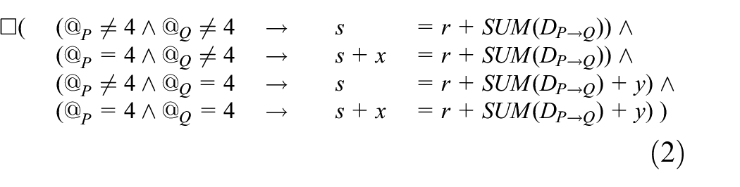
The formula for

Proof of Formula (2). We utilize standard induction on state number.
As the inductive base, we consider the initial state 0, in which
For the inductive step, we take an arbitrary state
Let us start with transition 〈P1〉. Before the transition, we have the formula true and
Precisely the same reasoning can be applied to transitions 〈P2〉 and 〈P5〉 … 〈P8〉.
Let us thus consider transition 〈P3〉. Before the transition, we have
The reasoning for transition 〈P4〉 is symmetric, so we leave it to the interested readers.
Furthermore, transitions 〈P1〉 and 〈P4〉 … 〈P8〉 are the same as the corresponding transitions for process
Before transition 〈Q3〉, we have
Having shown that no transition makes the formula false, we proved the inductive step, that is, that for any state
An analogous semantic proof can be conducted for Formula (3), so we leave it as an exercise for the interested readers. Instead, we exemplify how the deductive system,
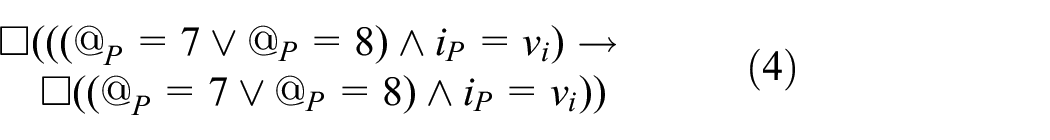
The same formula for process

The next formula, in turn, describes the termination of the main loop of process

An analogous formula is true for process

We are now ready to prove our main hypothesis: for any computation,
Proof
Combining Formulas (4)–(7), we get
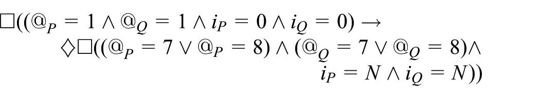
In other words, if the two processes start from their first instructions

Likewise, applying also the invariant for

Therefore, combining this with the invariant describing the dependency between

Finally, since any computation,
All in all, we hope to have illustrated that LTL is a sound and powerful formalism. It allows for capturing many intricacies of the dynamic behavior of concurrent programs. We will demonstrate its potential for deriving practically relevant formal guarantees for a routing protocol, like RPL.
Modeling RPL’s dynamic behavior
As we showed in the previous section, proving dynamic properties formulated in LTL for a concurrent program requires a model of a system running the program. In the case of a routing protocol, in particular RPL, the model should cover not only the algorithms constituting the protocol but also the impact of the environment in which they operate, notably the possible dynamics of nodes and links. The parts of the model describing the algorithms can be constructed based directly on algorithm descriptions, for example, the relevant RFCs in the case of RPL. They can also be built from existing protocol implementations, such as the aforementioned TinyRPL and ContikiRPL. The behavior of the environment, in turn, is typically modeled based on community knowledge.
In any case, the model has to satisfy two seemingly conflicting requirements. On one hand, its assumptions should not be oversimplified to a point that meeting them would be infeasible in the real world. Otherwise, the properties derived for the model would have little, if any practical relevance. On the other hand, its level of detail (i.e. complexity) should be under control. Otherwise, verifying even a simple property would be tedious, an example of which is arguably the proofs from the previous section. One of the main challenges in modeling is thus discovering which aspects can be simplified, how to perform the simplification, and what its practical consequences are.
A common first step to addressing this challenge is building a targeted model, including only those aspects of the protocol that are relevant to the behaviors of interest. If properly constructed, such a dedicated model does not preclude verifying other behaviors. On the contrary, this can be done by extending the model with new components or removing or replacing some existing ones.
Consequently, we will develop such a dedicated model here. More specifically, our model will target RPL’s DODAG construction and maintenance, which is the enabler of upward routing. To further limit its complexity, we will focus on a single instance and DODAG, because considering more would bring little new insight from the perspective of the tutorial. In addition, having completed the tutorial, the interested readers will be in position to develop the model appropriately. As a side note, the model will be a union of the models from our previous papers,6,7 further extended to cover extra aspects. This in particular implies that its key parts have been double-checked against ContikiRPL and TinyRPL to ensure that they are consistent and implementable.
We start by defining a state of the considered system, as required by the notion of computation in LTL. We then proceed to identifying possible state transitions. Finally, we formalize axioms describing the interplay between the two, which determine the dynamic behavior of the system.
System state
In line with the common terminology and previous sections, a system running a routing protocol such as RPL is defined in terms of nodes and links. Nodes host processes that execute the program implementing the algorithms constituting the protocol. Links are directed logical connections between pairs of nodes, thereby being a medium through which the processes can exchange packets. Together, they form a fixed directed communication graph,
Both nodes and links can be subject to failures, which disrupt their regular operation. A basic failure class in distributed systems is so-called crash-stop failures. 12 When a node crashes, it forever stops executing its program. Likewise, when a link crashes, it forever stops delivering packets. In contrast, the broadest class represents so-called Byzantine failures, in which failing nodes and links may behave arbitrarily and may even collude. Yet, hardly any practical routing protocol—RPL not being an exception—can tolerate nodes failing that way: routing protocols normally assume collaborative rather than malicious nodes. Similarly, nonmalicious links are normally considered.
Consequently, although one can adopt any failure class in LTL-oriented models, here we settle on a class that arguably covers a sufficient range of failures encountered in practice: so-called crash-recovery failures. In this class, a crashed node or link can recover: after recovery, a node starts its program from the beginning and a link resumes delivering packets. A node or link may thus alternate between being live and dead, which more faithfully models a real network. In this context, since the delivery of a packet between two neighbors depends on the liveness of these nodes and the links between them in some time span, to simplify formulations of our properties, we introduce a concept of “adjacency”: we say that two nodes are adjacent in a given LTL state iff in this state they are both live and the links between them in both directions are live as well.
Finally, it is important to note that having the communication graph,
Node state
Any global state has to contain for each node the data that the algorithms considered in the model require to run on this node. To this end, like in the example from the previous section, rather than modeling the node’s memory bytes, processor registers, and the like, we will model only values of relevant program variables. This approach reduces complexity and ensures the correct types of these variables. At the same time, it does not preclude modeling practical problems, like those related to storage limitations, if we chose to do so. For instance, if we wanted to verify the behavior of a protocol under a lack of packet buffers, we could introduce a variable representing a limited-size buffer pool. In our case, however, since the model targets RPL’s DODAG construction and maintenance, we limit our interest to the variables listed in Table 1 and corresponding to the concepts mentioned in the overview of the protocol.
Variables comprising the state of a node.
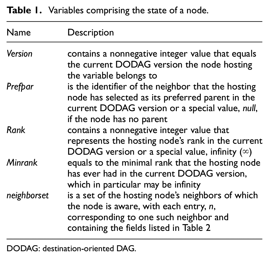
DODAG: destination-oriented DAG.
Variables
Fields of each entry,
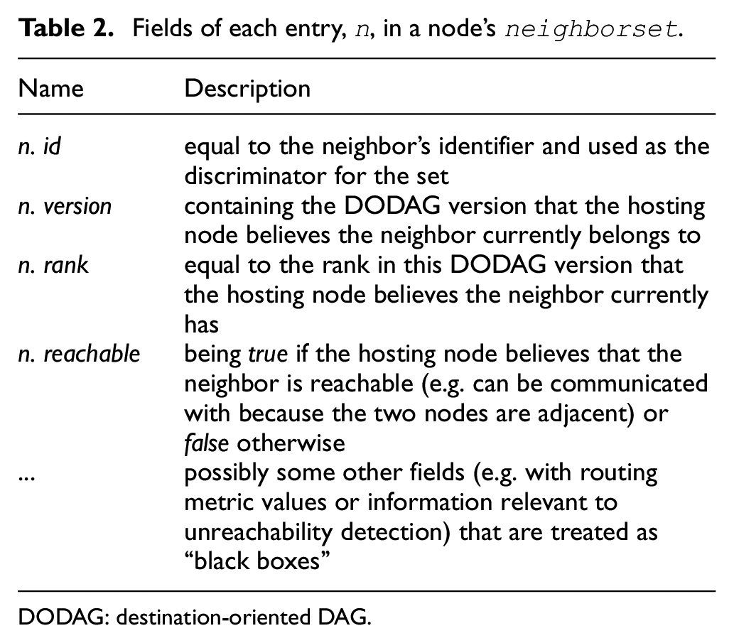
DODAG: destination-oriented DAG.
For any node
This brings us to another observation: any global state has to incorporate for each node information indicating whether the node is live or dead in this state. Accordingly, we will denote as
Finally, we assume for simplicity that the identifier of the DODAG root node is predefined and does not change in any computation. If necessary, this assumption can easily be dropped, though. For completeness, in Table 3, we also provide a summary of constants that a node in RPL utilizes.
RPL’s constants a node utilizes.
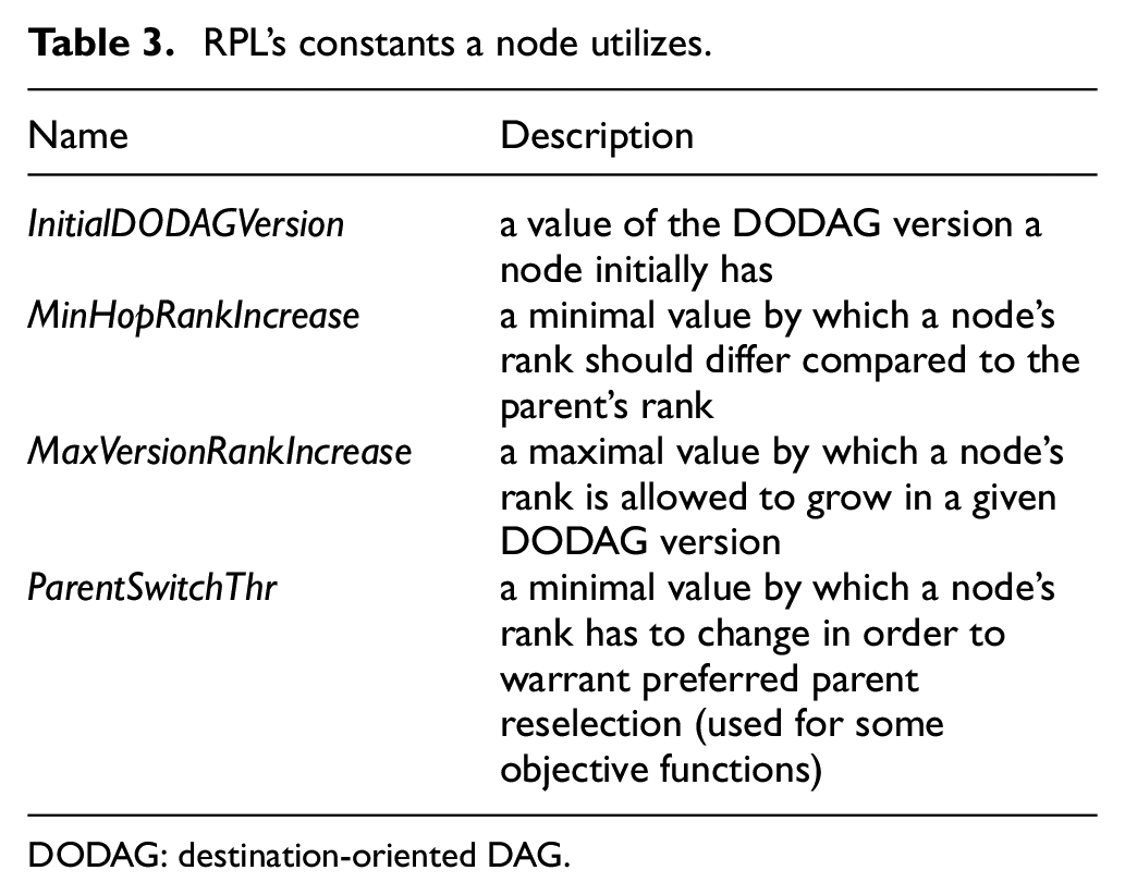
DODAG: destination-oriented DAG.
Link state
For each link, in turn, any global state has to contain packets that are in transit over the link in this state. Since link-layer communication between nodes is normally implemented by a stack of various low-lever protocols and operating system modules, being in transit may in practice describe several conditions. To give some examples, a packet in transit may be: in some buffer at some layer of the operating system of the transmitting node, in a buffer of the radio of this node, on air, in a buffer of the radio of the receiving node(s), or in one of the operating system buffers of these nodes. Consequently, to reduce the complexity of our model and at the same time cover all such situations, we represent all packets in transit over a given link like in the example from Listing 1: as a delivery multiset for this link, denoted
Furthermore, as highlighted previously, the core of DODAG maintenance is done mostly through ICMPv6 DIO messages, which carry the necessary information; DIS messages, in turn, are used mostly to solicit transmissions of DIO messages, whereas the purpose of RPL’s other messages is delivering functionality that already relies on upward routing, thereby being beyond the scope of our interest. Consequently, by properly abstracting the rules of DIO transmissions, neighbor reachability detection, and routing metric value maintenance—which we address shortly—we can limit our reasoning on DODAG construction to DIO messages. Accordingly, we assume that the delivery multiset,
What is more, we will be interested in DIO messages that can be received by a specific node. Therefore, for convenience, for each node
Variables comprising the state of a link.
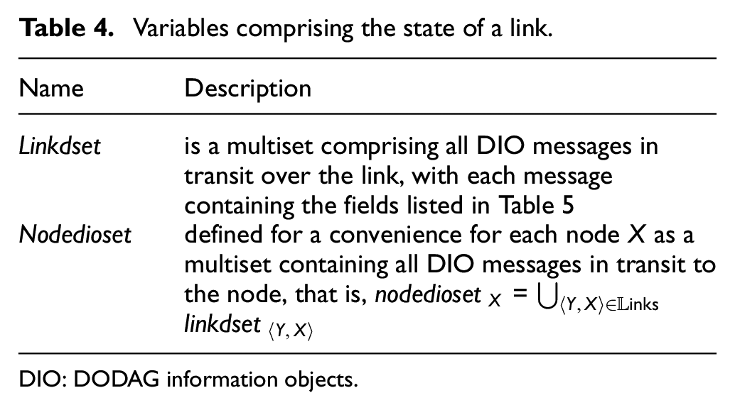
DIO: DODAG information objects.
Each DIO message,
Fields of a DIO message,

DODAG: destination-oriented DAG.
Finally, like a node, a link may be live or dead in any state. Therefore, we denote as
State transitions
To recap, in our model, a global state of the system incorporates information on which nodes and links are live, what packets are in transit over which links, and what values the local variables of the live nodes have. To be able to model an LTL computation, we need to define the possible transitions of the system between such states.
As a starting point, consider again the example from Listing 1 (with the control flow also visualized in Figure 3), in which a state transition was always due to one of the processes executing the instruction pointed by its program counter. Adopting that approach here would be problematic, though. Even if we provided code of a program implementing RPL, it would be rather voluminous, considering RPL’s specification and its implementations. This would remain true even if we limited the program to the aspects relevant only to the modeled variables, which we have confirmed empirically. In effect, any computation for the model would involve an excessive number of states, a large fraction of which would be completely immaterial to our reasoning and, yet, would have to be taken into account in our analyses. As an illustration, consider for instance Formula (2) from the aforementioned example. Even though it describes a simple invariant between two variables, it is composed out of four implications, whose sole purpose is addressing states with arguably irrelevant, temporal inconsistencies between the variables.
This observation hints at a potential solution to modeling state transitions: rather than to an execution of an individual instruction, a state transition can correspond to an execution of a logically related group of program instructions. For instance, in the example from Listing 1, instead of modeling the control flow of processes
This approach has to be further adapted to capture not only the studied algorithms but also the impact the environment has on them. In particular, in the example from Listing 1, we disregarded process and communication channel failures. To address this issue, we can model a state transition as a more general event. An event can correspond to an execution of a logically related group of program instructions, at a granularity even coarser than in the previous example, or some external phenomenon of the environment, including a crash or recovery of a processes or communication channel.
In general, apart from reducing model complexity, the event-based approach to describing state transitions has several advantages. It reflects the way protocol specifications are written, as they typically describe how protocols react to various events. It also matches many software architectures for low-power wireless systems, which are often event-driven. At the same time, without any special provisions, it can model asynchronous process execution and communication, which, as mentioned previously, are usually assumed for distributed algorithms. Likewise, with well-defined effects on the global state, it is by no means “less formal” than the program-counter-based approach from that section: events are simply higher level instructions that operate on the global state defined in the model.
Consequently, we employ the event-based approach here: a transition between two global system states is due to a particular event occurring. In the rest of this section, we thus list events triggered by the program running on the nodes and events caused by the environment. We give some intuition behind each event and discuss what components of the global system state it affects. The precise temporal properties for the events are in turn formalized in the next section.
Program-driven events
The events triggered by the program can occur only if the node they concern (i.e. the node executing RPL’s software) is live. They are simply responsible for modifying the node’s local variables and the delivery multisets of the links to and from the node, and are as follows:
DODAG version generation—occurs when RPL decides to build a new DODAG version; causes the executing node to set its variable
DODAG version adoption—takes place when RPL on the executing node decides to join a given DODAG version; again, causes the node to change its version to the given version number and to reset its variables
Parent and rank reselection—happens whenever RPL running on a node decides to change the node’s place in the present version of its DODAG; causes the node to set its
Neighbor entry addition—occurs independently of RPL, for instance, when an external protocol for routing adjacency maintenance discovers a node’s neighbor; causes a new entry,
Neighbor entry removal—also takes place independently of RPL, for example, when another protocol decides that a node’s neighbor is no longer worth monitoring; causes the entry,
Neighbor entry update of non-RPL fields—again, happens independently of RPL; for an existing entry,
DIO message reception—occurs when a packet containing a DIO message,
DIO message transmission—takes place if RPL running on a node decides to transmit a packet with a DIO message,
Each event thus indeed represents a logically related group of program instructions that forms a certain whole. Likewise, each of them can in principle be executed at any time, if the executing node is live. This explains why node program counters are not necessary in the global system state.
Environment-driven events
The events triggered by the environment are in turn as follows:
DIO message loss—occurs if a packet containing a DIO message,
Link start-up—takes place when a dead link goes up; causes the link to become live;
Link death—happens when a live link goes down; causes the link to become dead and may cause all or some of the messages in the link’s delivery multiset,
Node start-up—occurs when a dead node (re)starts; causes the node to become live and sets its local variables to their initial values (following the rules formalized in the next section);
Node death—takes place when a live node crashes; causes the node to become dead and makes the values of all its local variables undefined.
Whereas start-ups and crashes of particular nodes and links are typically defined per scenario, packet loss is an inherent feature of any low-power wireless network. For this reason, let us look more closely into modeling communication, especially since apart from packet loss, real-world communication may also exhibit packet corruption, duplication, and reordering, and, as emphasized previously, we strive to avoid any assumptions that would make our model unrealistic.
We start with packet corruption, which can manifest in a range of ways: from garbled bits to entire messages maliciously injected by an attacker. In all cases, the result is that a node receives a packet that has never been sent by any other node. As mentioned previously, routing protocols normally do not tolerate Byzantine failures and hence are not prepared to handle such spurious packets. Therefore, for protection, they—or, to be precise, entire network stacks they belong to—adopt a number of countermeasures at different layers: from checksums to various encryption schemes. In effect, core algorithms of the protocols typically assume that the problem of packet corruption is effectively dealt with elsewhere, which we formalize as the following property:
No creation: If node
As the subsequent phenomena, let us consider packet loss and duplication as they both affect packet delivery guarantees. For the communication channel between the two processes in the example from Listing 1, we assumed perfect delivery, under which any transmitted packet is delivered exactly once. In contrast, assuming perfect delivery in low-power wireless networks is simply unrealistic, especially for broadcast transmissions that are heavily utilized by RPL for packets with DIO messages. In other words, we must not ignore the two phenomena in our model.
A major issue when formalizing non-zero loss and duplication is again that we want to make as minimal and realistic assumptions as possible. For instance, accepting a certain percentage of packet loss is not sensible, especially since some low-power wireless links may have a truly low and variable quality. Therefore, we take an opposite approach, assuming that both loss and duplication are unknown for any link and may vary arbitrarily in time, which we formalize as follows:
Finite loss: If node
Finite duplication: If node
What the first property states is that if a node repeatedly forever transmits packets over a link, then the node on the other side of the link also repeatedly forever receives (some) packets over that link (recall the earlier explanation for the always eventually combination of temporal operators). There is no requirement as to which of the packets will actually be received or how many (consecutive) packets in such an infinite stream are allowed to be lost. In other words, there is no bound on packet loss and we cannot assume any specific chances of an individual packet being lost. However, thanks to being so extremely pessimistic, the property captures virtually all loss patterns encountered in the real world. Likewise, the second property expresses minimal assumptions on packet duplication. What it requires is only that the number of duplicates of a given packet be finite if the packet is transmitted a finite number of times, so that the reception of the packet’s duplicates ceases at some point (recall the explanation for the eventually always combination of temporal operators). In other words, no node forever keeps receiving the same packet (unless the packet is transmitted ad infinitum). The two properties are thus indeed extremely weak, which makes any conclusions derived based on them readily applicable in the real world. They were inspired by what is sometimes referred to as fair-loss delivery
12
but the original definition of that delivery model differs, though. Moreover, for the sake of simplicity, their present formulation implicitly assumes that nodes
As the final phenomenon, let us consider packet reordering. In principle, even packets transmitted over the same link may arrive in any order, depending on the policies at the link layer. Consequently, we do not assume any particular packet delivery order, again being pessimistic.
Axioms describing RPL’s operation
Given the definition of a global system state and the allowed transitions between such states, we are ready to formulate axioms describing when and how precisely specific transitions can take place. Considering the tutorial nature of this article, instead of the symbolic notation of LTL, we will continue using the natural language, like in the link properties from the previous section. In general, this is a common approach when analyzing distributed algorithms 12 as it greatly facilitates explaining the adopted reasoning and—when applied judiciously—need not make the reasoning “less formal.” To support this claim, we illustrate that in particular the previous properties for links can be expressed in the symbolic notation of LTL.
To this end, let us define the following predicates for DIO message transmissions and receptions:
With these predicates, the finite duplication property can be translated literally for any computation
Finite duplication:

The same is true for finite loss:
Finite loss:

Only the translation of the no creation property may arguably seem less straightforward:
No creation:

The reason for such a seemingly involved translation is that there is no standard operator in the symbolic notation that would allow in a given state of a computation for referring to past states. Consequently, to ensure that a reception of a packet over a link is preceded by a transmission of this packet over the link, the formulation utilizes the temporal operator until, which enforces the desired order of events. More specifically, it states that a given DIO message,
After this interlude, we can thus proceed to formulating the axioms describing RPL’s operation, as derived from its specification. They are divided into four groups that correspond to distinct pieces of functionality necessary given our focus on RPL’s DODAG formation and maintenance.
Control traffic axioms
The properties describing control traffic, that is, the way DIO messages are exchanged between neighboring nodes, can be formulated as follows.
They correspond directly to the previous link properties, albeit formulated in a manner that takes into account the way RPL utilizes DIO messages. More specifically, property CT1 corresponds to no creation, in addition defining how the values of fields
Routing adjacency maintenance axioms
As the next group, let us formulate properties describing routing adjacency maintenance, that is, the rules for maintaining nodes’ local
Accordingly, let us start with two properties that, while not formulated explicitly in RPL’s specification, can arguably be inferred from it.
Property RA1 states that any change to a node’s
Property RA2, in turn, formalizes consistency of those fields of
In contrast, when it comes to formalizing the actual tracking of neighbors and their adjacency, the specification contains no precise information, leaving this issue to external solutions. Yet, to be able to prove anything, we do have to make some assumptions on the behavior of such solutions. We formalize these assumptions as properties RA3 and RA4.
Property RA3 describes the rules of detecting unreachable neighbors. To be considered unreachable, a node’s neighbor, from some moment in time, has to permanently remain nonadjacent to the node (i.e. it has to be dead or its link with the node has to be down). This in particular means that neighbors that are temporarily nonadjacent need not be detected as unreachable—only ones that remain so for extended periods—in practice, depending on the timeouts of an actual failure detector. In other words, our assumptions on the failure detector are extremely weak, which makes any conclusions derived under them more broadly applicable in the real world. As a side note, our assumptions resemble those for what is known as eventually perfect failure detector in classic distributed algorithms.
12
Furthermore, regarding the marking of a neighbor entry as unreachable, the formulation of the property again does not impose any particular implementation: the marking can be done through the reachable flag or by removing the entry from the node’s
Property RA4 is symmetric to RA3 in that it considers reachable neighbors. Consequently, for brevity, we omit its discussion and proceed to formalizing another functionality.
DODAG versioning axioms
The next group of properties describes the management of DODAG versions. Unlike the previous one, this functionality does belong to RPL. Nevertheless, some of its aspects, notably those related to liveness, are still underspecified. Therefore, like previously, let us start with those properties that can arguably be inferred from RPL’s specification.
Property DV1 defines the initial value of a node’s
Property DV2 entails
Finally, property DV3 states that DODAG versions are monotonic. It is worth mentioning that while formalizing the intent of RPL’s designers, this property is only approximated but not guaranteed by the protocol. First, because of a limited width (8 bits) of
The next aspect concerns DODAG version generation. By and large, RPL’s specification leaves this issue open to implementers, notably when it comes to which node introduces a new version and when. In principle, we could assume that any node is allowed to start a new DODAG version. In practice, however, for management reasons, it is typically the root node that generates new versions, while the other nodes adopt them based on information from their
Related to DODAG version generation is adoption of generated versions, which is also the last aspect in the considered group of properties. Like previously, RPL’s specification contains virtually no requirements on when a node should adopt a new DODAG version. However, never demanding the node to do so precludes liveness: a DODAG version newly generated by the root node may never be adopted by any other node. On the other hand, aggressively forcing a node to adopt any new version it learns about may be an overkill. In search for a middleground, we thus oblige a node to change its
Objective function axioms
As the last group, we consider axioms describing the selection of a node’s preferred parent and rank in a DODAG version. As mentioned previously, this functionality is delegated to objective functions, such as OF0 55 and MRHOF. 56 In principle, they are treated by RPL as “black boxes.” Nevertheless, the protocol, sometimes implicitly, does define a few requirements on their results, which we gather into the following properties.
r≥n. r≤
Otherwise, the node adopts
Property OF1 defines the only events that affect a node’s
Property OF2 formalizes the dependency between a node’s
Property OF3 specifies that the root node’s
Finally, properties OF4 and OF5 are similar in that they describe rules for
Summary of lessons learned
All in all, the presented model does cover the aspects fundamental to studying the dynamic behavior of RPL’s DODAG construction and maintenance. Its system state includes all the elements that contribute to a DODAG at a particular moment: nodes, links, messages, versions, ranks, preferred parents, neighbor tables, adjacency, and routing metric values. At the same time, the state exhibits features characteristic to distributed systems, such as distribution of information among nodes and messages in transit, knowledge inconsistency between different nodes and even at a single node, communication with loss, duplication, and out of order delivery, and node and link failures and recoveries, to name a few prominent examples. The transitions between such states are also granular enough to model the evolution of these features in time. Finally, the rules for the transitions have been meticulously inferred from protocol descriptions, implementations, and community knowledge, so that the dynamic behavior they model comes close to what is observed in a real-world system, which we confirmed, among others, empirically.6–9
When presenting these issues, we aimed to illustrate typical problems that have to be faced when devising a formal model of a routing protocol. We highlighted the need for limiting complexity by focusing on features that are vital to the phenomena of interest. We showed how to model processing and communication, abstract algorithms comprising the protocol, and approach open issues and external solutions on which the protocol depends. Throughout our discussion, we emphasized the need for avoiding oversimplifying and overspecifying the model, which would otherwise make its behavior deviate from that observable in the real world, thereby limiting its potential for deriving practically relevant conclusions. Therefore, even though parts of the model can likely be reused out of the box for other routing protocols, we believe that it is the knowledge we aimed to share when presenting it that can guide the readers in their own modeling attempts.
What we have not discussed yet is in turn the iterative nature of a typical modeling process. In particular, the presented model is a result of over a dozen iterations that improved its various aspects. We illustrate how such adjustments can be performed at the end of the next section, as this requires some practice in verification.
Verifying hypotheses on RPL’s behavior
Given a model that describes the dynamic behavior of a routing protocol, we can formulate hypotheses regarding this behavior in various situations. We can then employ the LTL reasoning rules discussed previously to try to prove that a particular hypothesis holds for the model.
One possible outcome of such a verification attempt is a counterexample that identifies a specific scenario in which the hypothesis is violated. Analyzing such a counterexample we can conclude that the hypothesis is indeed false. In particular, many hypotheses that we formulated for RPL and that seemed intuitive at first turned out not to hold in the end. In effect, we were forced to reformulate them or abandon altogether, in both cases gaining new insights.
However, it may also be the case that we are missing some assumptions in our model or in the particular scenario the hypothesis considers. Armed with this knowledge, we may revise the model or make the considered scenario more specific. This reinforces our previous remark that a protocol verification process is typically iterative, alternating between modeling the protocol and (dis)proving hypotheses on its behavior, which is how our models of RPL emerged.
In any case, a product of the process that is at least equally important as a proof of a hypothesis is precise information on what properties of the model and the considered scenario are crucial for the hypothesis to hold. This knowledge can be utilized in practice at virtually all stages of protocol development. At the design stage, it can determine the architecture of the algorithms constituting the protocol and can drive their specification: one way or the other the information has to be put in the specification to facilitate building correct implementations. At the implementation and testing stages, it can help develop correct code: having the crucial properties explicitly formulated, it is much easier to maintain them in the code and to devise dedicated test scenarios. Finally, at the deployment stage, being aware of the assumptions on the scenarios in which the hypothesis holds gives more confidence in the reliability of the protocol in the target environment. In particular, in the case of RPL, even though the specification and implementations had already existed for several years, the aforementioned findings from our modeling and verification process still turned out relevant in practice,6,7 as we summarize further in the paper.
To this end, however, apart from an appropriate methodology and models, which were covered in the previous sections, one also requires suitable proof techniques. In particular, as mentioned previously, even if some hypotheses can be verified through (semi-)automated model checkers, manual proof techniques are typically necessary to generalize the results to other network configurations, protocol parameter settings, and the like. In this section, we thus give examples of the main techniques that we adopted and developed when proving various hypotheses for RPL. The techniques are discussed with selected hypotheses serving as running examples. Considering the tutorial nature of this article, the choice of the hypotheses aims to be illustrative rather than exhaustive. Nevertheless, we cover both safety and liveness properties.
Proving safety properties
Safety properties are often formulated as invariants that have to hold in all or in well-defined states of computations. A fundamental technique for proving an invariant in LTL is mathematical induction on time, that is, on the sequence of states representing a computation. This is precisely what we did when proving Formula (2) for the example from Listing 1. To conduct such a proof (cf. Figure 5), we take an arbitrary computation that is possible in the scenario that the property considers. Then, as the inductive base, we need to prove that the property holds in some state of the computation, typically but not necessarily the first state. Finally, as the inductive step, from the fact that the property holds in an arbitrary state (and all previous states) of the computation, we have to derive that it also holds in the next state. Depending on the property, rather than all states, we may consider only those that satisfy some specific criteria.
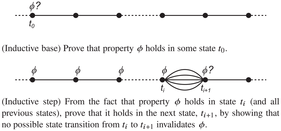
A typical approach of verifying an invariant by induction on time in an arbitrary computation.
Sample property
To illustrate the use of this technique, we will show the lower bound on ranks in RPL, that is, the fact that all ranks ever appearing in the system are at least
Lemma 1
Always, if a node is live, its variable rank and fields
Note that we named the property as “lemma” instead of “hypothesis.” This is to indicate that it is true. Irrespective of the naming convention, however, the property itself is not mentioned explicitly in RPL’s specification. Nevertheless, as we will demonstrate, it can be derived from our model of the protocol and hence from the specification itself. Having such an explicit formulation facilitates adding checks for the property in the code of RPL’s implementations. Considering that
Before delving into the proof, however, let us introduce some notation that will make our reasoning more succinct. More specifically, we define the following multisets:
We will denote the union of these multisets as
With this notation, Lemma 1 can be reformulated as follows:
For any state
Inductive proof
We are now ready of give a proof of the lemma.
Proof
Consider an arbitrary computation for our model.
The inductive base is the first state:
For the inductive step, we take an arbitrary state,
To this end, we analyze what effects each possible event has on
Node start-up. If the event corresponding to the transition of the system from state
Node death. If the event corresponding to the transition from state
Link start-up. A start-up of some link does not affect any of the multisets, and hence for all
Link death. Upon a death of some link
Neighbor entry addition. If the event corresponding to the transition from state
Neighbor entry update of non-RPL fields. This event does not affect any of the multisets, and thus for all
Neighbor entry removal. If the event during the transition from state
DIO message transmission. If the event causing the transition from state
DIO message reception. If the event is in turn a reception by node
DIO message loss. In the case of a DIO message loss, a DIO message is removed from linkdset of some link
Parent and rank reselection. If the event corresponding to the transition from state
DODAG version change (i.e. generation or adoption). The same dependency between the multisets occurs for a DODAG version change at some node
The proofs of the inductive base and the inductive step together confirm that in any state
Further examples of safety properties
To reinforce the claim that induction on the sequence of states constituting a computation is indispensable for proving safety properties, we give Lemmas 2 and 3, leaving their proofs with our model as an exercise for the interested readers.
Lemma 2
Always, if a node is live, its variable
Lemma 3
In any state, let
Lemma 2 is complementary to Lemma 1 in that it gives an upper bound on a node’s rank at any time. Its proof is simpler than the proof of Lemma 1 because fewer events directly affect a node’s variable
Lemma 3, in turn, bounds the DODAG version a node may have. Its proof is very similar to the presented one but for each event involving a DODAG version, we have to consider two cases: one in which the event affects the root node and the other in which a non-root node is affected. We will utilize the lemma in another proof in the next section.
Further examples of safety properties can also be found in our previous papers.6,7
Proving liveness properties
While proving safety often boils down to what we presented hitherto, proving liveness may be more intricate, as a particular technique may be strongly dependent on what precisely is being proved. The techniques that we will present in this and subsequent sections illustrate this claim, as they have been developed for proving liveness with regard to particular aspects of RPL. Since distance-vector routing protocols in general employ similar solutions, (some of) the techniques, possibly after some adaptation, may likely be reused also for other protocols. Nevertheless, by no means do we consider the techniques a complete repertoire for proving liveness. On the contrary, we envision that their prospective users will encounter problems that will require novel approaches. Therefore, our main goal is to discuss carefully selected examples so as to provide the readers with some directions and inspiration for attacking such problems.
We start with local liveness properties, normally involving a single node or a couple of nodes. We then exemplify proving global properties, referring to the entire node population.
Example of a local liveness property
Liveness properties that involve a small number of nodes can often be derived from the properties comprising the model without any sophisticated techniques. Occasionally, even (semi-)automated model checkers can help to this end. More advanced examples, in turn, include proofs by contradiction or some form of induction. Since we will illustrate the use of contradiction in a proof of a global liveness property in the next section, in this section we discuss an example of custom induction for proving a local liveness property, formulated as Lemma 4. As a side note, we will use this lemma to prove the aforementioned global liveness property.
Lemma 4
Always, if a node’s
In short, the lemma combines the properties describing the adoption of new DODAG versions, notably properties DV5 and DV3, into something useful: the premises of the lemma are the same as of property DV5 but the conclusions are stronger. It states that if a node is aware of a DODAG version that is newer than its own one and that has already been adopted by a stable neighbor (i.e. one with which the node has a reliable link for a sufficiently long time), then eventually the node will abandon its current DODAG version and join a new one: either the one adopted by the neighbor or some yet newer. The difficulty in proving the lemma is that nothing in the model (and in RPL’s specification) forces a node to adopt a specific DODAG version and hence it can potentially change its version multiple times. Worse yet, so can its neighbors in the meantime. We will use induction to show that irrespective of the number of such changes that may be necessary, the node’s DODAG version will forever reach or exceed the given neighbor’s version.
Proof
Consider an arbitrary computation for our model, an arbitrary node
To conduct this proof, we will use induction on the difference between
As the inductive base, let us take
For the inductive step, in turn, we assume that the lemma holds for all
More specifically, from the premises of the lemma, we know that in state
If
If, in turn,
These two cases thus conclude the inductive step. The proofs of the inductive base and the inductive step, combined with the fact that the initial state,
Example of a global liveness property
Let us return to Lemma 4, namely to its formulation, which exemplifies that a liveness property is typically conditional: given some assumptions, a desired effect (“something good”) will occur. As the lemma describes a local property, its assumptions are simply copied from a property defined in our model (DV5). However, this need not always be the case. In particular, for a global property, one normally needs some additional assumptions on the entire system. Let us thus first demonstrate how such assumptions can be formalized. As a running example, we aim to prove a global property in which the desired effect is—informally—the following: “all nodes eventually join (adopt) a DODAG version generated by the root node.”
To start with, we need the aforementioned universal assumptions stating that the communication graph,
Pursuing this line of reasoning further, we may observe that learning about a DODAG version depends not only on the existence of links between nodes but also on whether the nodes and links are live, and hence we introduce assumptions A1 and A2. Finally, the root node may generate multiple DODAG versions, some of which will not (and need not) be adopted by all nodes, but we do want to have some guarantees nevertheless. We deal with this problem by formalizing DODAG version generation by the root node as assumption A3.
The formulation of assumptions A1–A3 borrows from a standard approach to analyzing eventually consistent distributed algorithms:49,51 assume that the system becomes and remains quiescent (the “eventually always” in A1–A3) and show it will eventually become consistent as well. Demanding system quiescence, assumptions A1–A3 may seem strong at first, but this impression is wrong if they are interpreted correctly. The “eventually always” should be interpreted as “from some moment in time for a sufficiently long period,” where “sufficiently long” depends on the actual timings, which are not modeled in LTL. In particular, propagating a DODAG version in RPL can in practice take as little as a few hundred milliseconds, even in large networks. Furthermore, “all nodes/links” in A1 and A2 could be relaxed to a spanning tree, which in addition need not have all its parts simultaneously live. This, however, would require an extended discussion, which we would like to avoid as being immaterial. Consequently, we adopt this standard, quiescence-based formulation of the assumptions and formalize our target global liveness property as Lemma 5. Since assumptions A1–A3 are not universal but rather specific to the particular operational scenario considered in the lemma, we state them explicitly in the lemma body.
Lemma 5
If assumptions A1, A2, and A3 hold, then eventually always, each node has its
Even disregarding its assumptions, the fact that the lemma is a global liveness property should be apparent. It describes the expected behavior of all nodes. Its desired effect is in turn the adoption by the nodes of the last DODAG version generated by the root node.
One of the main challenges in proving such a property is that it is often impossible to conduct the proof on a snapshot of the system (i.e. a single state of a computation involving the system). On the contrary, since the configuration of the system is dynamic, such proofs usually analyze what happens in multiple specific consecutive states of the computation. Identifying a sequence of such important states need not be straightforward. In our experience, however, an effective approach is to match the analysis in the proof with the way the desired effect spreads in the system.
In particular, a good initial heuristic is trying to prove such a property by induction on hop count in the communication graph,

The node’s hop counts from the root node in the sample network from Figure 1.
To conduct such a proof, we start by taking an arbitrary computation that satisfies the assumptions of the property: in the case of Lemma 5, assumptions A1–A3. Then, as the inductive base, we need to prove that the property holds at the initiating nodes, for which the hop count is 0: for our lemma, the root node. Typically, this requires finding a state,

Verifying a liveness property by induction on hop count in the communication graph.
Proof
For our model, consider an arbitrary computation that satisfies assumptions A1, A2, and A3.
From assumption A1, there exists a state of the computation,
Let, thus,
We will use induction on the hop count from the root node to prove that, for any
To this end, as the inductive base, consider
Accordingly, assume that a transition of the system from some state
For the inductive step, assume that for all nodes that are up to
To this end, consider an arbitrary node,
To begin with, from the definition of
First, node
Second, from
Since, as mentioned previously, from
If
If, in turn,
To recap, in both cases, there exists a state,
Since node
Combining the inductive base and the inductive step with the fact that the communication graph formed by nodes and links is finite and connected, and hence the maximal distance in hops of any node from the root node is bounded, we can conclude that eventually always each node in the considered computation has its
Devising custom non-trivial inductive orders
While induction on hop count may be a good starting point when trying to prove a global liveness property, it need not work in all cases. As an illustration, let us consider Hypothesis 1, whose simplified version was originally subject of our previous work. 7
The desired effect in the hypothesis concerns RPL’s fundamental functionality: building a DODAG that allows all nodes to perform upward routing to the root node. To be precise, for a DODAG to be formed, every non-root node must have its
We leave to the interested readers’ discretion an attempt to prove Hypothesis 1 by induction on hop count in the communication graph. In summary, under an additional assumption, which we will return to shortly, it is relatively straightforward to prove the inductive base and show that if all nodes within
This observation hints at the main problem with hop count as the inductive order for a proof of Hypothesis 1: parent selection by the objective function depends on dynamic routing metric values and hence may not reflect the nodes’static hops from the root. In particular, if at some point a neighbor with a larger hop count offers a node a better potential rank (
There are two problems with this relation, though. First, the subgraph induced by the nodes’ links to preferred parents need not be acyclic, which is necessary for a graph describing an order. Second, the node’s preferred parents can change in subsequent states of a computation, whereas inductive reasoning requires an order to be fixed. As a result, we cannot utilize the preferred parent relation as an order for induction.
To propose an alternative order, let us introduce a concept of what we dubbed best ever parents (BEPs). A node’s BEP is defined for a given DODAG version and is the node’s current or former preferred parent, whose selection gave the node the smallest rank ever in this particular DODAG version for the first time. In our notation, this is the node’s
An illustration of the best ever parent (BEP) idea.
Given this concept, in any state,
Lemma 6
Always, the best-ever-parents (BEP) graph for any DODAG
Lemma 7
The best-ever-parents (BEP) graph for any DODAG version,
The proofs of these lemmas (merged into a single lemma) can be found in our earlier paper. 7 The interested readers should likely be able to recreate them. To give some hints, proving Lemma 6 requires showing two properties, which in both cases can be done by contradiction: first, that the BEP graph never contains any cycle and second, that any path in the graph ends at the DODAG root. Proving Lemma 7, in turn, boils down to observing that a node’s minrank is an integer with a lower-bound formalized in Lemma 1 and hence cannot decrease indefinitely.
From our perspective, what is more important than the details of the proofs themselves is the implications of the lemmas. Lemma 6 essentially states that, in any state of any computation, the BEP graph for any DODAG version is acyclic and hence can represent a partial order of nodes. Lemma 7 implies in turn that from some state of any computation this order is fixed. Combining the lemmas, we can thus conclude that the order induced by the BEP graph is suitable for proofs by mathematical induction. An example of a possible BEP graph, and the induced order, for the sample DODAG from Figure 1 is presented in Figure 9.
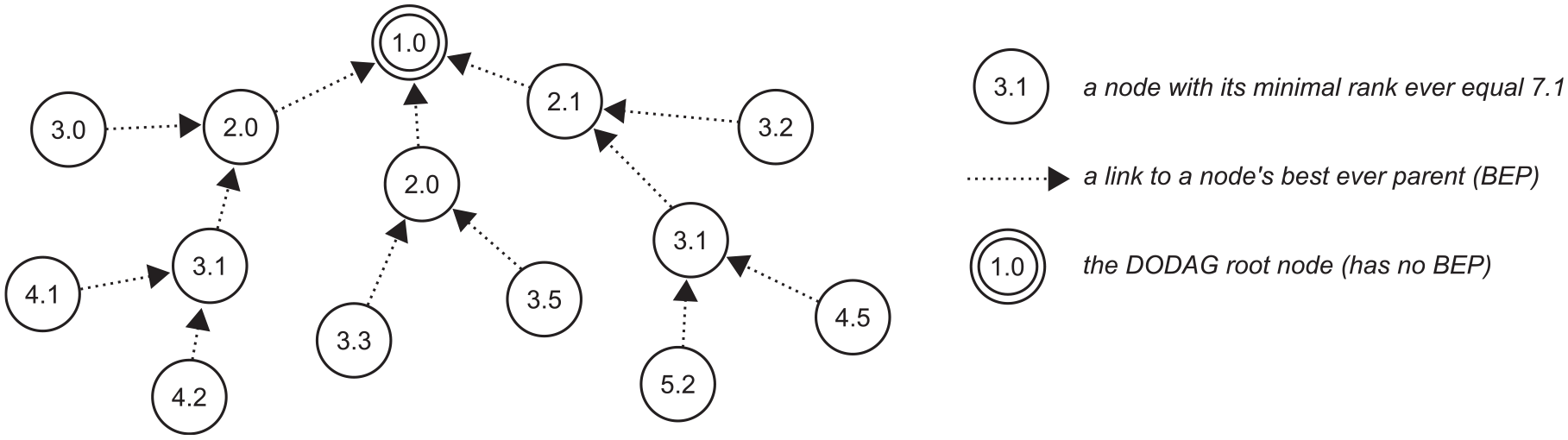
An illustration of the best ever parents in the sample DODAG from Figure 1.
Such a proof proceeds roughly in the same manner as in the previous techniques but involves some extra steps. Like usual, we start by taking an arbitrary computation that satisfies the assumptions of the property that is being proved. Then, we consider a specific DODAG version,
As we demonstrate next, following this approach allows for proving what we tried to express in Hypothesis 1: that RPL is able to build and maintain a DODAG. From a broader perspective, in turn, our discussion hitherto exemplifies how one can devise a dedicated inductive order to match the way the desired effect of a global liveness property spreads in the system. Finally, the presented theoretical concept of BEPs also has practical applications, such as monitoring DODAG health for generating DODAG versions, especially for custom routing metrics. 7
Working with hypotheses and assumptions
Given a technique advertised as suitable for proving that nodes in RPL are capable of choosing and keeping finite ranks, we will proceed slightly differently than previously. Rather than just giving the target lemma, we will present the entire process of formulating and proving it. We will propose an initial version of the lemma by adding two assumptions and adapting Hypothesis 1 to the devised proof technique. While proving the lemma, we will be reformulating it and introducing further assumptions. This will illustrate what we mentioned previously: that a formal verification process is normally iterative. All in all, this section is meant to complete the suite of skills that we believe are necessary to begin modeling and verifying routing protocols on one’s own.
Formulating an initial hypothesis
We start with the missing assumption mentioned in the previous section. More specifically, let us observe that the only way for a non-root node to get its
What A4 states is that for each neighbor set entry representing a node’s neighbor that belongs to the same DODAG version as the node, has itself advertised a finite rank recently, and is considered by the node as reachable, the node is guaranteed to obtain a finite rank, irrespective of the objective function and values of the routing metrics employed. Demanding in this case that a potential rank be finite, albeit possibly very high, is a sensible assumption, further backed by what RPL’s aforementioned implementations ensure. Although we could adopt a weaker one, this would require a deeper discussion, which is not strictly relevant and is thus avoided here for brevity.
The second issue is that the current formulations of the OF properties, and our model in general, completely abstract out routing metrics. However, changes to their values do affect calculated potential ranks and hence the nodes’ ranks. Therefore, to continue treating routing metrics as “black boxes” while being able to reason about their changes, we introduce assumption A5.
Assumption A5 stems from RPL’s recommendation regarding the function for computing potential ranks: the function should be additive. At the same time, through function
Given A4 and A5 we are ready to revise the false Hypothesis 1, reformulating it into Hypothesis 2. Apart from including the two assumptions, the new hypothesis explicitly foresees that more may yet be necessary. In addition, it considers only the members of the final BEP tree,
Refining the hypothesis
If we introduced yet another assumption, A6, proving Hypothesis 2 would be relatively easy, which we leave as an exercise to the interested readers.
Assumption A6 makes it possible for the routing metrics for a neighbor—or, given assumption A5, the corresponding values of
However, assumption A6 is too strong to be satisfiable in practice: routing metrics rarely remain fixed at their minimal values; on the contrary, usually they change dynamically. Consequently, for our work to have any real-world relevance, this assumption must be weakened, which implies allowing routing metrics to grow. However, considering the previous argument, if this growth were unbounded, then it would be possible for a node to always lack a neighbor entry satisfying OF5(f). We thus have to somehow limit the growth of the routing metric values.
To this end, for each neighbor entry,
We encourage the interested readers to come up with these dependencies of
Having addressed the liveness of prefpar and rank reselection as well as the dynamics of routing metric values, it seems we may be ready to formulate and attempt to prove a variant of our target hypothesis, Hypothesis 2, which has stronger conclusions than Hypothesis 2.
Proof
For our model, consider an arbitrary computation that satisfies assumptions A1–A5 and A6. From assumptions A1–A3 and Lemma 5, there exists a state,
As the inductive base consider the root node, whose depth,
To show the inductive step, in turn, consider an arbitrary non-root node,
We start by showing that eventually always, whenever
From
From
From
(iv) There exists a state,
(v) From the fact that node
Consider state
Since
As the next step, we will prove that node
To recap, we have proved that eventually whenever
A7 simply states that a node always selects as its preferred parent the neighbor that offers it the lowest potential rank. This can be the node’s BEP or another neighbor, if during a particular reselection that neighbor offers the node a smaller rank than the BEP. For node
However, instead of concluding the entire proof, let us observe that despite not forcing the objective function to select a node’s BEP as the preferred parent, A7 may still be too constraining. This is because it always requires the objective function to select a preferred parent that offers the node the lowest rank. Since always aiming at the best preferred parent may result in frequent parent changes, there exist objective functions, such as MRHOF, 56 that explicitly rely on more freedom in the choice of a node’s preferred parent. This freedom is realized by employing the aforementioned hysteresis, which prohibits the node from switching its preferred parent unless this is sufficiently beneficial, that is, unless the potential rank offered by the new parent is lower than the node’s current rank by more than a threshold, denoted ParentSwitchThr. Consequently, to capture such freedom in our model, we have to relax A7, replacing it with assumption A7.
While A7—and hysteresis in general—gives much more freedom when selecting preferred parents, it may lead to their suboptimal choices if ParentSwitchThr> 0. To explain, under the previous assumptions, if selecting a node’s BEP as
Apart from taking A7 instead of A6, our previous reasoning remains valid otherwise, verifying which we leave to the interested readers. In other words, the inductive step holds with
Combining the inductive base and the inductive step with the fact that the final BEP tree,
To emphasize this fact, we present the final hypothesis that we have just proved as Lemma 8.
Lemma 8
If assumptions A1, A2, A3, A4, A5, A6″, and A7 hold, then eventually always, each member of the final BEP tree,
Closing remarks
The previous reasoning showed how by iterating on hypotheses and their assumptions we can prove a key property for RPL. In particular, given Lemma 8, we can further show that the final BEP tree eventually always covers all nodes, that is, eventually always
Lemma 9
If assumptions A1–A5, A6″, and A7′ hold, then eventually always, the final BEP graph contains no isolated nodes, that is,
Finally, by combining Lemmas 6, 7, 8, and 9, we can also conclude what follows.
Lemma 10
If assumptions A1–A5, A6″, and A7′ hold, then eventually always, all nodes have their
Lemma 10 constitutes the essence of RPL’s DODAG maintenance from the perspective of the considered model and hence reinforces our claims about the potential of the presented techniques for verification of dynamic behaviors of routing protocols. What is equally important, however, is the insight we obtained while proving the lemma. In particular, we identified assumptions under which the lemma holds, found issues in RPL’s specification that may require extra treatment by implementers, and gave explicit dependencies between some key configuration parameters, which are not mentioned in the specifications. This knowledge can be employed to improve the reliability of RPL-based systems, both in general and in specific deployment scenarios.
Summary of lessons learned
Overall, in this section, using our model of RPL, we aimed to illustrate how one can verify properties describing dynamic behaviors of a routing protocol. We covered both canonical types of properties that are distinguished in program verification: safety and liveness. Safety properties typically correspond to invariants that have to hold in all or in well-defined states of computations in a system. We thus demonstrated a common approach to checking an invariant, which involves analyzing all possible transitions between global system states and proving that none of them violates the considered invariant. Liveness properties, in turn, often describe various forms of progress that a system is expected to make under specific assumptions. We argued that a good verification heuristic is trying to match a proof of such a property with the way the desired effect it describes spreads in the system, giving a few examples substantiating this argument. We also exemplified that particularly involved properties may require devising custom inductive orders. Finally, we illustrated the iterative nature of a normal verification process, which includes formulating a hypothesis, attempting to verify it, revising its assumptions or the model, and repeating everything, possibly more than once.
Furthermore, while it was not our main goal in this tutorial, we specifically selected the properties serving as our examples so that together they cover a key aspect of RPL’s functionality for upward routing: DODAG construction and maintenance. In particular, we formulated invariants bounding rank values and DODAG versions, progress properties for version adoption, and, finally, lemmas formalizing RPL’s ability to continuously reselect node ranks and parents in an evolving network, so that globally they correspond to a DODAG. Equally important as the properties themselves is the insight presented while proving them, like the identified assumptions under which they hold or undocumented dependencies between RPL’s configuration parameters they entail. In this light, we also tried to discuss practical relevance of individual properties, in particular, where they were not formulated in or even implied by RPL’s specification. We recapitulate them shortly. As a final remark, since RPL’s upward routing is an application of classic distance-vector routing technique, some of the properties we proved can be applied directly to other routing protocols based on this technique.
In contrast, we did not even aspire to show what one might expect as a “complete repertoire” of verification techniques for dynamic behaviors of routing protocols. We simply believe that no such concept exists. Instead, however, we strove to touch upon all verification aspects that we believe to be relevant, to give sufficiently illustrative examples, and to put everything into perspective so as to demonstrate the behaviors of a key piece of functionality incorporated into routing protocols. We hope that this knowledge will help the readers to start their own verification attempts.
Applying the results in practice
Throughout the tutorial, we gave several examples of how the particular results or insights can be applied in practice. In fact, the presented analyses were actually inspired by real-world problems that we encountered when deploying RPL. The covered techniques were in turn developed to address these problems, which ultimately resulted in fixing existing protocol implementations and adjusting their configurations based on our findings. We are unable to precisely discuss those results here. Nevertheless, we do provide highlights and pointers, so that the interested readers can explore these topics at their discretion.
One example was invalid responses of the two open-source RPL implementations to crashes of border routers (DODAG roots): 8 an entire network either completely collapsed or entered a state of increased resource consumption without actually detecting the failure. It was not clear whether this behavior was due to bugs in the implementations or emergent properties of the protocol itself. Using the techniques covered in this tutorial, we proved that, by design, RPL is able to handle crashes of border routers or, in general, network partitions, and derived formal conditions that have to be met to this end. 6 In particular, a variant of Lemma 1 was necessary in the proofs, and they involved further safety and global liveness properties. Since some of those conditions had never been explicitly formulated, the implementations simply did not satisfy them, and hence operated incorrectly.
Another example was nonstandard, albeit intuitive route construction criteria taking into account energy consumption, for which the two implementations completely collapsed. 7 Like previously, using the techniques presented here, we derived conditions for provably correct route formation and identified potentially imprecise statements in RPL’s specification, which may lead to invalid protocol configurations. In particular, variants of the assumptions used to prove Lemma 8 were one of the results of the process. The insight obtained when deriving these assumptions allowed us to formulate practical guidelines for RPL’s implementers, adopters, and designers of future objective functions and route optimization criteria. 7
What these two examples also illustrate is that the aforementioned risks involved in deploying a routing protocol—even one having mature and widely adopted, and hence seemingly reliable implementations—may indeed be considerable and have profound consequences. They also reinforce the previous claim that guarantees on the behavior of the protocol can help manage such risks, which is more and more relevant with the surging real-world deployments of IoT technologies for controlling physical processes.
Conclusion
To sum up, routing is fundamental technology underlying today’s Internet and will likely remain crucial in the emerging IoT. Routing protocols are examples of what is referred to as “complex systems.” In particular, they operate on many nodes in a distributed fashion, normally leave some issues open to implementers, rely on external solutions providing side functionalities, involve multiple configuration parameters, and interact with their environment. As a result, predicting their behavior is often nontrivial. At the same time, especially in the context of industrial IoT, where nodes collaboratively control physical processes, overall system dependability requires, among others, precise guarantees on the behavior of the routing protocols employed.
In this tutorial, we illustrated how such guarantees can be derived formally. As a running example of a routing protocol, we adopted RPL, the current de jure standard for low-power wireless networks, which are one of the key communication technologies in IoT. The underlying formalism was in turn based on LTL, which allowed us to focus on actual dynamic behavior (i.e. the evolution) of a system rather than just properties of static system snapshots. After a brief introduction to RPL and LTL, we showed how a routing protocol such as RPL can be modeled in the selected formalism and how such a model can be utilized for verifying the dynamic behavior of the protocol.
In the modeling part, we aimed to illustrate the common problems that one is likely to encounter when devising a formal model of a routing protocol. To avoid excessive complexity, we concentrated on the core, albeit sufficiently broad subset of RPL’s DODAG construction and maintenance functionality. We showed how to model processing and communication, abstract algorithms comprising the protocol, and deal with open issues and external dependencies. In our discussion, we emphasized the need for avoiding oversimplifying and overspecifying the model, which would otherwise limit the real-world applicability of the conclusions from verification attempts involving the model.
In the verification part, in turn, we strove to demonstrate how safety and liveness properties—the two types of properties crucial for distributed algorithms and hence routing protocols—can be proved with our model of RPL. To this end, we discussed a few techniques, including invariance checking, contradiction, and induction on various orders. We also exemplified how to approach devising a custom inductive order, which may be necessary for proving more involved properties. Finally, we demonstrated the iterative nature of a typical verification process, including hypothesis formulation, possibly failed proof attempts to identify missing or incorrect assumptions, and gradual hypothesis refinement to make it truly realistic and relevant in practice.
In terms of content, although this was not our main objective, we did cover several key areas of RPL’s DODAG construction and maintenance functionality. For example, we proved fundamental bounds on nodes’ ranks and DODAG versions in a correctly functioning system, liveness of DODAG version dissemination, and guarantees on the global rank and parent assignment and upkeep. What the tutorial also highlighted as being as important as these results was the insight obtained when producing them. This included assumptions necessary for the proved properties to hold, dependencies between seemingly unrelated configuration parameters, and other issues that are not mentioned explicitly or are simply missing in RPL’s specification.
All in all, we believe that this tutorial and its pointers can be of value for both theoretical and practical purposes. From the practical perspective, the presented results can themselves be utilized when extending RPL or designing new distance-vector routing protocols, writing specifications, implementing them, and configuring for particular deployment scenarios. The aforementioned real-world problems with RPL that inspired our work are a good example. From the theoretical perspective, in turn, the tutorial may guide building new models or retargeting the presented one and proving additional properties. For instance, further use of our methodology, not covered here for the sake of brevity, led to deriving guarantees on RPL’s fault tolerance, control traffic behavior, and the impact of asymmetric links; nevertheless, many issues, like the performance of routing adjacency maintenance solutions, downward routing, or multicast, are still open. As our deployment experiences and previous research underlying this tutorial indicate, such knowledge is valuable when aiming at highly dependable systems, as in industrial IoT.
Footnotes
Acknowledgements
The authors would like to thank Agata Janowska for providing early feedback on some parts of this paper. The authors are also grateful to the anonymous reviewers whose comments have helped to improve the quality of this paper.
Handling Editor: Peio Lopez Iturri
Declaration of conflicting interests
The author(s) declared no potential conflicts of interest with respect to the research, authorship, and/or publication of this article.
Funding
The author(s) disclosed receipt of the following financial support for the research, authorship, and/or publication of this article: This article was supported by the National Science Center (NCN) in Poland under grant no. 2019/33/B/ST6/00448. Its contents also partly draw from our earlier work, supported by the National Center for Research and Development (NCBR) in Poland under grant no. LIDER/434/L-6/14/NCBR/2015.