Research on error compensation in the process of geomagnetic sensor measurement

Abstract

The geomagnetic sensor is a kind of highly sensitive sensor, which is easy to be interfered with by the outside in the process of measurement. To solve this problem, the author uses the least square method to estimate the gain value and sensitivity product value of the amplification circuit of the geomagnetic sensor and explores the solution of the bias voltage of the geomagnetic sensor by using the ellipsoid fitting model. By analyzing the error sources of the geomagnetic sensors in the measurement process, the error compensation model covering various error factors is constructed. All parameters of the error compensation model are obtained by fitting the experimental data of the turntable. After several experiments with different attitude angles, the validity of the compensation model is verified, and the measurement accuracy of the roll angle is improved, which meets the requirements of roll angle measurement.

Introduction

The geomagnetic field is the inherent basic physical field of the earth. Geomagnetic intensity exists at any place in the near-earth space, and the intensity and direction will change with the longitude, latitude, and height, but in a relatively short time and a small space, the difference is not significant.^1,2 Based on the characteristics of the geomagnetic field, the three-axis geomagnetic sensor can measure the projection of geomagnetic vector on the carrier coordinate system, so as to obtain the attitude of the carrier and provide technical support for navigation control. Attitude measurement technology is the key part of positioning and navigation technology. In geomagnetic navigation, three-axis geomagnetic sensor is the core component of attitude measurement system. Three-axis geomagnetic sensor has the characteristics of small volume, low cost, high precision, strong shock resistance, and overload ability. It is widely used in many fields such as guidance and control, navigation, and magnetic measurement.^3–8

In practical application, geomagnetic sensor will be interfered by its own factors and external factors, resulting in errors in the measurement results. Due to the limitation of material and technology, the sensor will produce non-orthogonal error and DC bias in the manufacturing process, and the installation error will occur in the installation process. The soft magnetic error and hard magnetic error will be caused by the interference magnetic field in itself and environment. Therefore, the three-axis output of geomagnetic sensor cannot appear as a sphere, but an ellipsoid, so the optimal estimation of parameters in the relationship between input and output is needed for attitude measurement. At present, the method of parameter calibration and error compensation of geomagnetic sensor is usually divided into attitude angle based ⁹ and attitude independent calibration,^10,11 which will introduce external equipment, which will increase the investment of actual cost. Therefore, this article explores the calibration and error compensation algorithm based on attitude angle.

Many scholars have studied the error compensation in the process of geomagnetic sensor measurement, for example, Wang et al. ¹² established standard least square method, stable least square method, constrained least square method, and truncated least square method to analyze the sensor measurement data, which can effectively compensate the magnetic measurement. However, the least square method is too complex to solve the DC bias of geomagnetic sensor, so, it is not easy to establish the solution model; Crassidis et al. ¹³ uses the Extended Kalman filter and Unscented Kalman filter to calibrate the magnetic sensor error, but the filtering has limitations and cannot cover all error factors; Liu et al. ¹⁴ compensated the error of geomagnetic sensor by establishing differential magnetic field and compensated soft magnetic error and hard magnetic error by nonlinear least square method and changing the installation mode of three-axis geomagnetic sensor, but the compensation algorithm does not cover all error factors, and the operation process requires high requirements; Kok and Schön ¹⁵ used the inertial navigation system (accelerometer and gyroscope) to assist the geomagnetic sensor correction and used the jet plane flight experiment to verify the effectiveness of the algorithm. However, the calculation process is complex and not easy to solve; Vasconcelos et al. ¹⁶ proposed a fitting algorithm based on maximum likelihood estimation, which can directly obtain the error compensation matrix to compensate the magnetic measurement distortion. However, the iterative method is too complex to obtain the compensation matrix and the efficiency is not high; Wu and Shi ¹⁷ proposed an approximate quadratic maximum likelihood estimation based on four subjective functions to replace magnetic measurement calibration for magnetic measurement compensation. However, the calculation process is too complex and the efficiency is low. Liu et al. ¹⁸ calibrated the three-axis magnetic sensor by establishing particle swarm optimization algorithm, which effectively reduced the magnetic measurement accuracy, but the work efficiency was low, and the actual engineering application was low. Compared with the improved least square method, ¹⁹ maximum likelihood estimation fitting algorithm, ¹⁷ and Kalman filter algorithm, ²⁰ this method establishes a complete error model, and the calculation process is simpler; compared with the use of inertial navigation system, ¹⁵ external magnetic field, ¹⁴ and intelligent optimization algorithm,^21,22 this method can reduce the input of experimental steps and cost, and better meet the engineering application. Through the three-axis non-magnetic turntable test, this method can control the roll angle error within 2° and achieve the laboratory calibration accuracy under the same conditions and effectively improve the roll angle measurement accuracy. At the same time, it can improve the magnetic measurement accuracy by an order of magnitude.

The motivation of this article is that the product of the sensitivity of the sensor and the gain of the amplifier circuit is calibrated by using the least square method, and the bias voltage of the sensor is solved by using the ellipsoid fitting, and then, the error compensation matrix is solved by using the attitude angle experiment. The least square method can effectively solve the influence of installation error and non-orthogonal error on the sensor calibration process. The ellipsoid fitting method can effectively solve the influence of hard magnetic error and bias voltage on the sensor calibration process. Both of them can be used in the sensor calibration process at the same time, which can effectively improve the accuracy of sensor output parameter calculation. The method has low requirements for experimental environment and simple operation process, which is suitable for practical engineering application.

The rest of this article is as follows: the second section mainly introduces the calibration principle of the geomagnetic sensor; the third section analyzes the error source of the geomagnetic sensor and establishes the error compensation model based on the error analysis; the fourth section calculates the error compensation model through experiments and obtains the compensation effect of the compensation model through the measurement of roll angle. Finally, the fifth section summarizes the conclusion.

Calibration principle

In the process of geomagnetic navigation control, the x-axis of the geomagnetic sensor can measure the angle between the carrier axis and the geomagnetic vector, and the other two axes can measure the rolling attitude of the carrier and transmit the attitude of the carrier to the linkage rudder, which can control the flight direction and distance of the carrier. The direct output of the geomagnetic sensor is the voltage value, which cannot directly give the angle information needed in the geomagnetic navigation. It can be converted by the mathematical model shown in the following formula

$$V_x=S_x{K}_{x}B\cos {\theta }_{\mathrm{Bx}}+V_{x{90}^{°}}$$

(1a)

$$V_y=S_y{K}_{y}B\cos {\theta }_{\mathrm{By}}+V_{y{90}^{°}}$$

(1b)

$$V_z=S_z{K}_{z}B\cos {\theta }_{\mathrm{Bz}}+V_{z{90}^{°}}$$

(1c)

In the above formula, Vx, Vy, and Vz are the direct output voltage values of X-axis, Y-axis, and Z-axis of geomagnetic sensor; Vx90°, Vy90°, and Vz90° are output voltage values of three-axis sensor when local magnetic sensor is in non-magnetic environment; Sx, Sy, and Sz are sensitivity of three-axis geomagnetic sensor; Kx, Ky, and Kz are the gain values of amplification circuit corresponding to three-axis geomagnetic sensor; B is the geomagnetic field strength; and θBx, θBy, and θBz are the angles between the three axes of the geomagnetic sensor and the geomagnetic vector. Generally, in the circuit design of the geomagnetic sensor measurement system, the three axes of the geomagnetic sensor are connected in series with their respective amplification circuits, so the product of the sensitivity and the gain value of the amplification circuit can be regarded as a variable L, that is, the expression is L = S*K. The sensitivity and zero drift value of the geomagnetic sensor are the attributes of the sensor. The gain value of the amplifier circuit is related to the selection of the amplifier circuit. The geomagnetic field strength B is the inherent attribute of the geomagnetic field, which can be calculated by the World Magnetic Model (WMM).

The final goal of sensor calibration is to get more accurate variable L and zero drift value, which can reduce the influence of system error for subsequent attitude test. It can be seen from formula 1 that the direct output voltage value of the geomagnetic sensor is a cosine function of the angle between the sensor sensitive axis and the geomagnetic vector. From the image characteristics of cosine function, the following formula can be obtained, which can be expressed by mathematical model as follows

$$L_x=\frac{V_{\mathrm{bx}max}-V_{\mathrm{bx}min}}{2B},V_{x{90}^{°}}=\frac{V_{\mathrm{bx}max}+V_{\mathrm{bx}min}}{2}$$

(2a)

$$L_y=\frac{V_{\mathrm{by}max}-V_{\mathrm{by}min}}{2B},V_{y{90}^{°}}=\frac{V_{\mathrm{by}max}+V_{\mathrm{by}min}}{2}$$

(2b)

$$L_z=\frac{V_{\mathrm{bz}max}-V_{\mathrm{bz}min}}{2B},V_{z{90}^{°}}=\frac{V_{\mathrm{bz}max}+V_{\mathrm{bz}min}}{2}$$

(2c)

In the above formula, Vbxmax and Vbxmin are the maximum and minimum values of the sensor output when the x-axis of the geomagnetic sensor rotates one circle around the axis perpendicular to the geomagnetic vector; Vbymax and Vbymin are the maximum and minimum values of geomagnetic sensor output when y-axis rotates around the axis perpendicular to the geomagnetic vector; Vbzmax and Vbzmin are the maximum and minimum output values of the geomagnetic sensor when the z-axis rotates around the axis perpendicular to the geomagnetic vector.

In the actual calibration experiment, it is not easy to determine the direction of geomagnetic vector, so it is necessary to analyze θBx, θBy, and θBz. Taking the North-Sky-East coordinate system as the basic coordinate system, represented by O-NSE, and taking the geomagnetic sensor coordinate system as the carrier coordinate system and represented by O-XYZ, the angle between the three axes of the geomagnetic sensor and the geomagnetic vector is analyzed. During the calibration experiment of geomagnetic sensor, the longitude, latitude, and altitude of the experimental site can be measured by satellite. Using the latest International Geomagnetic Reference Field (IGRF13) given by the International Association of Geomagnetism and Aeronomy (IAGA), the tilt angle and deflection angle of geomagnetic vector of the experimental site in the North Tianshan coordinate system can be obtained, which are expressed by I and D (the magnetic inclination angle is positive in the horizontal plane. the magnetic declination is positive from north to west). The mathematical model is expressed as

$$B_g=\left[\begin{array}{ccc}B\cos I\cos D\hfill & B\sin I\hfill & -B\cos I\sin D\hfill \end{array}\right]$$

(3)

In the above formula, Bg represents the direction and size of the geomagnetic vector. Any attitude of the carrier in the North-Sky-East coordinate system can be transformed by the method shown in Figure 1:

Figure 1.

Coordinate system transformation process.

In Figure 1, the geomagnetic sensor coordinate system was completely coincident with the North-Sky-East coordinate system at first. β, α, and γ were the rotation angles around Y-axis, Z-axis, and X-axis, respectively. Then, the attitude of carrier coordinate system in the North-Sky-East coordinate system was expressed as follows

$$X=N\cos \alpha \cos \beta +S\sin \alpha -E\cos \alpha \sin \beta$$

(4a)

$$\begin{array}{c}Y=N(-\sin \alpha \cos \beta \cos \gamma +\sin \beta \sin \gamma )+\hfill \\ S\cos \alpha \cos \gamma +E(\sin \alpha \sin \beta \cos \gamma +\cos \beta \sin \gamma )\hfill \end{array}$$

(4b)

$$\begin{array}{c}Z=N(\sin \alpha \cos \beta \sin \gamma +\sin \beta \cos \gamma )-\hfill \\ S\cos \alpha \sin \gamma +E(-\sin \alpha \sin \beta \sin \gamma +\cos \beta \cos \gamma )\hfill \end{array}$$

(4c)

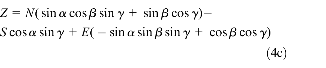
It can be seen from the three formulas that the projection of geomagnetic vector on the three axes of the North-Sky-East coordinate system is BN, BS, and BE, which can be expressed by mathematical expression as BN = BcosIcosD, BS = BsinI, and BE = –BcosIsinD. If they are brought into the above formula, the projection of geomagnetic vector on the three axes of the carrier coordinate system can be obtained. The mathematical model is expressed as follows

$$B_X=B\cos I\cos \alpha \cos (D-\beta )+B\sin I\sin \alpha$$

(5a)

$$\begin{array}{c}{B}_Y=-B\cos I\sin \alpha \cos \gamma \cos (D-\beta )-\hfill \\ B\cos I\sin \gamma \sin (D-\beta )+B\sin I\cos \alpha \cos \gamma \hfill \end{array}$$

(5b)

$$\begin{array}{c}{B}_Z=B\cos I\sin \alpha \sin \gamma \cos (D-\beta )-\hfill \\ B\cos I\cos \gamma \sin (D-\beta )-B\sin I\cos \alpha \sin \gamma \hfill \end{array}$$

(5c)

By transforming the Sum-to-product Identities of the above formula, the following formula can be obtained

$$B_X=B{A}_x\sin (\alpha +{\lambda }_x)$$

(6a)

$$B_Y=-B{A}_{\mathrm{yz}}\sin (\gamma +{\lambda }_{\mathrm{yz}})$$

(6b)

$$B_Z=-B{A}_{\mathrm{yz}}\cos (\gamma +{\lambda }_{\mathrm{yz}})$$

(6c)

In the above formula

$$A_x=\sqrt{{\cos }^{2}I{\cos }^2(D-\beta )+{\sin }^{2}I}$$

(7a)

$${\lambda }_x=\mathrm{arctg}\frac{\cos (D-\beta )}{\tan I}$$

(7b)

$${\lambda }_{\mathrm{yz}}=\mathrm{arctg}\frac{\sin \alpha \cos (D-\beta )-\tan I\cos \alpha }{\sin (D-\beta )}$$

(7c)

$$\begin{array}{c}{A}_{\mathrm{yz}}=\hfill \\ \sqrt{{(\cos I\sin \alpha \cos (D-\beta )-\sin I\cos \alpha )}^2+{\cos }^{2}I{\sin }^2(D-\beta )}\hfill \end{array}$$

(7d)

Another mathematical expression of variable L and zero-drift value can be obtained by taking equation (6) back to equation (2), as shown in the following formula

$$L_x=\frac{V_{xmax}-V_{xmin}}{2B{A}_x},V_{x{90}^{°}}=\frac{V_{xmax}+V_{xmin}}{2}$$

(8a)

$$L_y=\frac{V_{ymax}-V_{ymin}}{2B{A}_{\mathrm{yz}}},V_{y{90}^{°}}=\frac{V_{ymax}+V_{ymin}}{2}$$

(8b)

$$L_z=\frac{V_{zmax}-V_{zmin}}{2B{A}_{\mathrm{yz}}},V_{z{90}^{°}}=\frac{V_{zmax}+V_{zmin}}{2}$$

(8c)

In the above formula, Vxmax and Vxmin are the maximum and minimum output values of the geomagnetic sensor when the X-axis rotates around the Z-axis; Vymax and Vymin are the maximum and minimum values of the geomagnetic sensor’s Y-axis rotation around the X-axis; Vzmax and Vzmin are the maximum and minimum values of the geomagnetic sensor’s Z-axis rotation around the X-axis.

Error compensation and modeling of geomagnetic sensor

Because the geomagnetic sensor in the manufacturing process, there are manufacturing errors, and affected by the environment, installation accuracy and other factors, inevitably produce errors. The error can be divided into three categories according to the causes: ²³

1. The sensor itself. The sensor is affected by the manufacturing materials, manufacturing technology and manufacturing environment, which will cause the deviation between the sensitivity and zero drift value of the sensor and the standard value. The three sensitive axes cannot be completely orthogonal to each other in the manufacturing process; One is installation design error, including installation error and gain error of amplifier circuit;

2. Installation design error, including installation error and gain error of amplifier circuit;

3. Magnetic measurement error, including hard magnetic error and soft magnetic error.

Error analysis and modeling of geomagnetic sensor

Due to the limitation of installation technology, there is a certain deviation between the installation position of the three-axis geomagnetic sensor and the ideal position, which can be represented in Figure 2.

Figure 2.

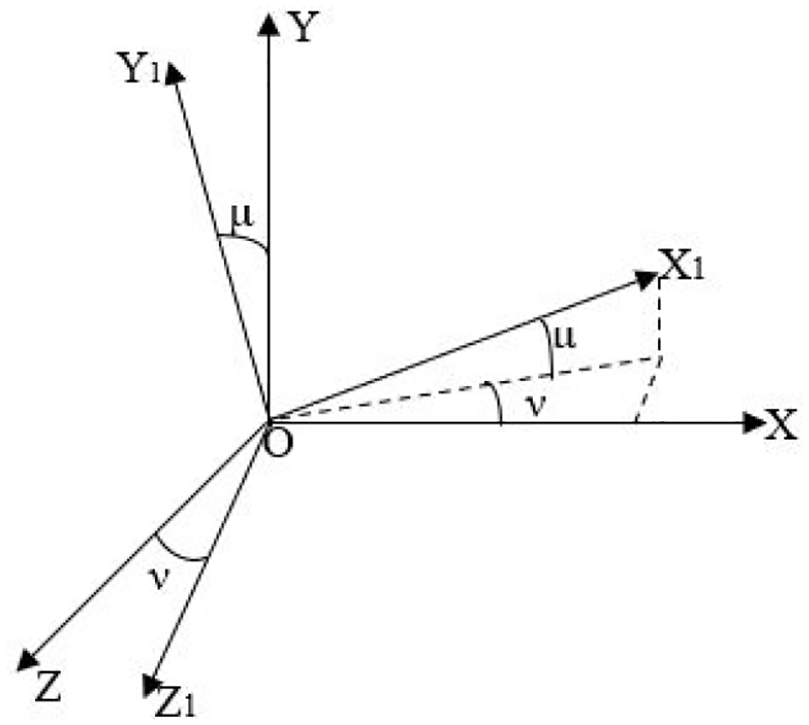
Installation error model.

In Figure 2, the coordinate system O-XYZ is the ideal installation position of the sensor three axes, the coordinate system O-X1Y1Z1 is the actual installation position of the sensor three-axis, and μ and ν are the installation error angles. The angle between the X1 axis and the OXZ plane is μ; the angle between the projection of the X1-axis in the OXZ0 plane and the X-axis is ν; the angle between the Z1 axis in the OXZ plane and the Z-axis is ν; the Y1-axis is perpendicular to the OX1Z1 plane and the included angle with the Y-axis is μ. The position of the coordinate system O-X1Y1Z1 in the coordinate system O-XYZ is expressed as follows

$$\left[\begin{array}{c}{X}_1\hfill \\ \multicolumn{1}{c}{Y_1}\\ \multicolumn{1}{c}{Z_1}\end{array}\right]=\left[\begin{array}{ccc}\cos \mu \cos \nu \hfill & \sin \mu \hfill & -\cos \mu \sin \nu \hfill \\ \multicolumn{1}{c}{-\sin \mu \cos \nu }& \cos \mu \hfill & \sin \mu \sin \nu \hfill \\ \multicolumn{1}{c}{\sin \nu }& 0\hfill & \cos \nu \hfill \end{array}\right]\left[\begin{array}{c}X\hfill \\ \multicolumn{1}{c}{Y}\\ \multicolumn{1}{c}{Z}\end{array}\right]$$

(9)

In equation (9), X, Y, and Z are the ideal geomagnetic intensity measured by the geomagnetic sensor triaxial, and X1, Y1, and Z1 are the geomagnetic intensity measured by the geomagnetic sensor with installation error.

The three axes of the geomagnetic sensor are orthogonal in design. However, in practical application, the three sensitive axes of the sensor cannot be strictly orthogonal, which leads to non-orthogonal error. The non-orthogonal model is shown in Figure 3.

Figure 3.

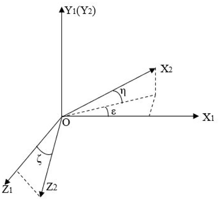
Non-orthogonal model of three-axis geomagnetic sensor.

In Figure 3, the coordinate system O-X1Y1Z1 is the ideal sensor triaxial distribution, the coordinate system O-X2Y2Z2 is the actual sensor triaxial distribution, and ζ, η and ε are the non-orthogonal error angles between the three axes of the geomagnetic sensor. The angle between X2 axis and OX1Z1 plane is η, the included angle between the projection of X2 axis in plane OX1Z1 plane and X1 axis is ε, and the included angle between Z2 axis and Z1 axis in OX1Z1 plane is ζ. The non-orthogonal error model shown in the above figure can be expressed as

$$\left[\begin{array}{c}{X}_2\hfill \\ \multicolumn{1}{c}{Y_2}\\ \multicolumn{1}{c}{Z_2}\end{array}\right]=\left[\begin{array}{ccc}\cos \epsilon \cos \eta \hfill & \sin \eta \hfill & -\sin \epsilon \cos \eta \hfill \\ \multicolumn{1}{c}{0}& 1\hfill & 0\hfill \\ \multicolumn{1}{c}{\sin \zeta }& 0\hfill & \cos \zeta \hfill \end{array}\right]\left[\begin{array}{c}{X}_1\hfill \\ \multicolumn{1}{c}{Y_1}\\ \multicolumn{1}{c}{Z_1}\end{array}\right]$$

(10)

In equation (10), X2, Y2, and Z2 are the geomagnetic intensity measured by the three axes of the geomagnetic sensor with installation error and non-orthogonal error.

The sensitivity of sensor sensitive axis is the inherent attribute of sensor, which is used to measure the relationship between output and input. No two sensors have the same sensitivity. Usually in the design of measurement circuit, the sensitive axis of the sensor is connected with an amplifier circuit in series. The purpose of the amplification circuit is to enlarge the output by several times, so as to observe the change of the output of the sensor. In mathematics, when analyzing the calculation error, it is impossible to distinguish the sensitivity error from the gain value error of the amplifier circuit. Therefore, the product of the sensitivity and the gain value of the amplifier circuit is analyzed as a variable, that is, the variable L in the previous section. The error model of the variable L is shown in the following formula

$$\left[\begin{array}{c}{X}_3\hfill \\ \multicolumn{1}{c}{Y_3}\\ \multicolumn{1}{c}{Z_3}\end{array}\right]=\left[\begin{array}{ccc}{l}_x\hfill & 0\hfill & 0\hfill \\ \multicolumn{1}{c}{0}& l_y\hfill & 0\hfill \\ \multicolumn{1}{c}{0}& 0\hfill & l_z\hfill \end{array}\right]\left[\begin{array}{c}{X}_2\hfill \\ \multicolumn{1}{c}{Y_2}\\ \multicolumn{1}{c}{Z_2}\end{array}\right]$$

(11)

In equation (11), X3, Y3, and Z3 are the geomagnetic intensity measured by the three axes of the geomagnetic sensor with installation error, non-orthogonal error, and sensitivity error, and Lx, Ly, and Lz are the variable L errors corresponding to the three axes of the geomagnetic sensor.

The soft magnetic error is caused by the external magnetic field induced by the geomagnetic sensor itself, which affects the output value of the geomagnetic sensor. In the calibration experiment of geomagnetic sensor, the static calibration of fixed location is adopted, the magnitude and direction of external magnetic field do not change, and the response of soft magnetic material can be regarded as linear change without lag. Assuming that the matrix of soft magnetic coefficient is expressed by Cr, the output value of the three axes of geomagnetic sensor is expressed as follows:

$$\left[\begin{array}{c}{X}_4\hfill \\ \multicolumn{1}{c}{Y_4}\\ \multicolumn{1}{c}{Z_4}\end{array}\right]=C_r\left[\begin{array}{c}{X}_3\hfill \\ \multicolumn{1}{c}{Y_3}\\ \multicolumn{1}{c}{Z_3}\end{array}\right]=\left[\begin{array}{ccc}{c}_{11}\hfill & c_{12}\hfill & c_{13}\hfill \\ \multicolumn{1}{c}{c_{21}}& c_{22}\hfill & c_{23}\hfill \\ \multicolumn{1}{c}{c_{31}}& c_{32}\hfill & c_{33}\hfill \end{array}\right]\left[\begin{array}{c}{X}_3\hfill \\ \multicolumn{1}{c}{Y_3}\\ \multicolumn{1}{c}{Z_3}\end{array}\right]$$

(12)

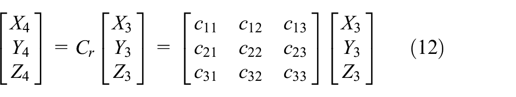
In equation (12), X4, Y4, and Z4 are the geomagnetic intensities with installation error, non-orthogonal error, variable L error and soft magnetic error.

Different from the soft magnetic error, the hard magnetism error is constant, which is the excess magnetic field removed from the geomagnetic field in the environment. The hard magnetism error model can be expressed as

$$\left[\begin{array}{c}{X}_5\hfill \\ \multicolumn{1}{c}{Y_5}\\ \multicolumn{1}{c}{Z_5}\end{array}\right]=\left[\begin{array}{c}{X}_4\hfill \\ \multicolumn{1}{c}{Y_4}\\ \multicolumn{1}{c}{Z_4}\end{array}\right]+\left[\begin{array}{c}{P}_1\hfill \\ \multicolumn{1}{c}{P_2}\\ \multicolumn{1}{c}{P_3}\end{array}\right]$$

(13)

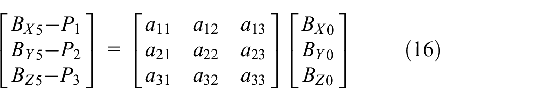
In equation (13), P1, P2, and P3 are the sum of the hard magnetism error and zero drift error of the three axes of the geomagnetic sensor, while X5, Y5, and Z5 are the geomagnetic intensity with installation error, non-orthogonal error, variable L error, soft magnetism error, and bias measured by the three axes of the geomagnetic sensor.

The error model of geomagnetic sensor can be obtained by introducing equations (10)–(13) into equation (9), as shown in the following formula

$$\left[\begin{array}{c}{X}_5\hfill \\ \multicolumn{1}{c}{Y_5}\\ \multicolumn{1}{c}{Z_5}\end{array}\right]=C_r{C}_l{C}_f{C}_a\left[\begin{array}{c}X\hfill \\ \multicolumn{1}{c}{Y}\\ \multicolumn{1}{c}{Z}\end{array}\right]+\left[\begin{array}{c}{P}_1\hfill \\ \multicolumn{1}{c}{P_2}\\ \multicolumn{1}{c}{P_3}\end{array}\right]$$

(14)

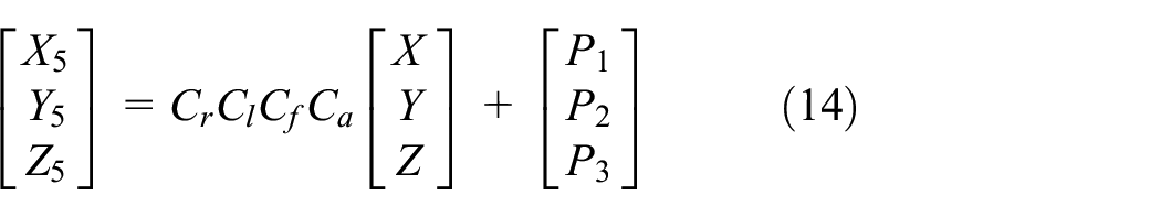
In equation (14), Cr, Cl, Cf, and Ca are soft magnetic error coefficient matrix, variable L error coefficient matrix, non-orthogonal error coefficient matrix, and installation error coefficient matrix, respectively. Since Cr, Cl, Cf, and Ca are 3 × 3 matrices, their product must also be 3 × 3 matrices, and equation (14) can be rewritten into the following formula

$$\left[\begin{array}{c}{X}_5\hfill \\ \multicolumn{1}{c}{Y_5}\\ \multicolumn{1}{c}{Z_5}\end{array}\right]=\left[\begin{array}{ccc}{a}_{11}\hfill & a_{12}\hfill & a_{13}\hfill \\ \multicolumn{1}{c}{a_{21}}& a_{22}\hfill & a_{23}\hfill \\ \multicolumn{1}{c}{a_{31}}& a_{32}\hfill & a_{33}\hfill \end{array}\right]\left[\begin{array}{c}X\hfill \\ \multicolumn{1}{c}{Y}\\ \multicolumn{1}{c}{Z}\end{array}\right]+\left[\begin{array}{c}{P}_1\hfill \\ \multicolumn{1}{c}{P_2}\\ \multicolumn{1}{c}{P_3}\end{array}\right]$$

(15)

Therefore, the error model of three-axis geomagnetic sensor can be expressed by 12 parameters in the above formula.

Error compensation and modeling of geomagnetic sensor

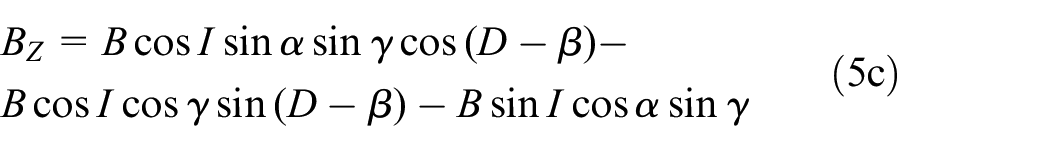
For the convenience of description, equation (15) can be rewritten as follows

$$\left[\begin{array}{c}{B_X}_5-P_1\hfill \\ \multicolumn{1}{c}{{B_Y}_5-P_2}\\ \multicolumn{1}{c}{{B_Z}_5-P_3}\end{array}\right]=\left[\begin{array}{ccc}{a}_{11}\hfill & a_{12}\hfill & a_{13}\hfill \\ \multicolumn{1}{c}{a_{21}}& a_{22}\hfill & a_{23}\hfill \\ \multicolumn{1}{c}{a_{31}}& a_{32}\hfill & a_{33}\hfill \end{array}\right]\left[\begin{array}{c}{B_X}_0\hfill \\ \multicolumn{1}{c}{{B_Y}_0}\\ \multicolumn{1}{c}{{B_Z}_0}\end{array}\right]$$

(16)

In equation (24), BY0 and BZ0 have nothing to do with roll angle γ, so make γ be zero. BY0 and BZ0 can be obtained from equation (5)

$$B_{Y0}=-B\cos I\sin \alpha \cos (D-\beta )+B\sin I\cos \alpha$$

(17a)

$$B_{Z0}=-B\cos I\sin (D-\beta )$$

(17b)

After rolling a projectile with a roll angle of 0, it will rotate the angle of φ around the X0 axis of the geomagnetic sensor. The following formula can be obtained from equation (16)

$$\begin{array}{c}\left[\begin{array}{c}{B}_{X6}-P_1\hfill \\ \multicolumn{1}{c}{B_{Y6}-P_2}\\ \multicolumn{1}{c}{B_{Z6}-P_3}\end{array}\right]\hfill \\ =\left[\begin{array}{ccc}{a}_{11}\hfill & a_{12}\hfill & a_{13}\hfill \\ \multicolumn{1}{c}{a_{21}}& \sin (\arccos a_{21})\cos (\phi +\mathrm{arctg}\frac{a_{23}}{a_{22}})\hfill & \sin (\arccos a_{21})\sin (\phi +\mathrm{arctg}\frac{a_{23}}{a_{22}})\hfill \\ \multicolumn{1}{c}{a_{31}}& -\sin (\arccos a_{31})\sin (\phi +\mathrm{arctg}\frac{a_{33}}{a_{32}})\hfill & \sin (\arccos a_{31})\cos (\phi +\mathrm{arctg}\frac{a_{33}}{a_{32}})\hfill \end{array}\right]\left[\begin{array}{c}{B}_{X0}\hfill \\ \multicolumn{1}{c}{B_{Y0}}\\ \multicolumn{1}{c}{B_{Z0}}\end{array}\right]\hfill \end{array}$$

(18)

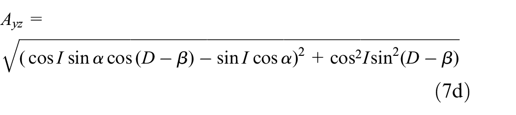
The mathematical expressions of BY6 and BZ6 can be obtained by substituting equation (17) into the above formula, as shown in the following formula

$$\begin{array}{c}\multicolumn{1}{c}{B_{Y6}-P_2=}\\ \multicolumn{1}{c}{a_{21}{B}_{X0}+\mathrm{BA}\sin (\arccos a_{21})\cos (\phi +\mathrm{arctg}\frac{a_{23}}{a_{22}}-\kappa )}\end{array}$$

(19a)

$$\begin{array}{c}\multicolumn{1}{c}{B_{Z6}-P_3=}\\ \multicolumn{1}{c}{a_{31}{B}_{X0}-\mathrm{BA}\sin (\arccos a_{31})\sin (\phi +\mathrm{arctg}\frac{a_{33}}{a_{32}}-\kappa )}\end{array}$$

(19b)

In the above formula

$$\begin{array}{c}A=\hfill \\ \sqrt{{\cos }^{2}I{\sin }^2(D-\beta )+{[-\cos I\sin \alpha \cos (D-\beta )+\sin I\cos \alpha ]}^2}\hfill \end{array}$$

(20)

$$\kappa =\mathrm{arctg}\frac{\sin (D-\beta )}{\sin \alpha \cos (D-\beta )-\tan I\cos \alpha }$$

(21)

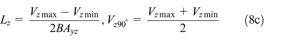
The relationship between the output and input of the geomagnetic sensor can be obtained by introducing equation (19) into equation (1). When the roll angle φ rotates from 0° to 360°, it can be seen from equation (19) that the Y-axis and Z-axis of the geomagnetic sensor will output a maximum value and a minimum value. The mathematical model is expressed as follows

$$V_{\mathrm{wy}max}=L_y(a_{21}{B}_{X0}+\mathrm{BA}\sin (\arccos a_{21})+P_2)+V_{y90}$$

(22a)

$$V_{\mathrm{wy}min}=L_y(a_{21}{B}_{X0}-\mathrm{BA}\sin (\arccos a_{21})+P_2)+V_{y90}$$

(22b)

$$V_{\mathrm{wz}max}=L_z(a_{31}{B}_{X0}+\mathrm{BA}\sin (\arccos a_{31})+P_3)+V_{z90}$$

(23a)

$$V_{\mathrm{wz}min}=L_z(a_{31}{B}_{X0}-\mathrm{BA}\sin (\arccos a_{31})+P_3)+V_{z90}$$

(23b)

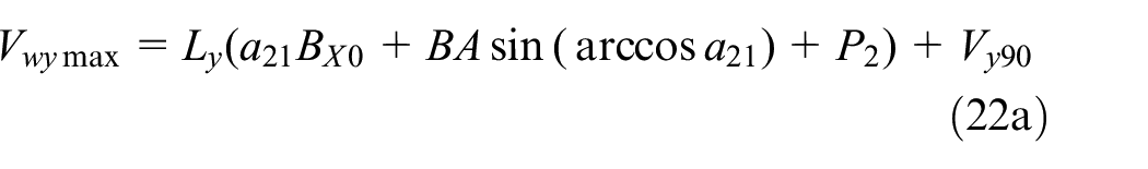
After simple mathematical transformation, the following formula can be obtained

$$V_{\mathrm{wy}max}+V_{\mathrm{wy}min}=2L_y{a}_{21}{B}_{X0}+2L_y{P}_2+2V_{y90}$$

(24)

$$V_{\mathrm{wy}max}-V_{\mathrm{wy}min}=2L_y\mathrm{BA}\sin (\arccos a_{21})$$

(25)

In equations (24) and (25), Ly, a21, P2, and Vy90 are constant values for the same sensor, and Vwymax and Vwymin are the maximum and minimum values of the output voltage of the geomagnetic sensor Y-axis. α and β in A and Bx0 can be regarded as independent variables, Vwymax + Vwymin and Vwymax —Vwymin can be seen as contributing variables. From equations (24) and (25), it can be seen that Vwymax + V_wymin and Vwymax −Vwymin are the first-order functions of Bx0 and B × A, respectively. By using the least square method to fit the equations (24) and (25), Ly × a21 and Ly × sin(arccos a21) can be obtained, which can solve the specific solution of Ly. It can be expressed as follows

$$L_y=\sqrt{{(L_y{a}_{21})}^2+{(L_y\sin (\arccos a_{21}))}^2}$$

(26)

After simple mathematical transformation, the following formula can be obtained

$$V_{\mathrm{wz}max}+V_{\mathrm{wz}min}=2L_z{a}_{31}{B}_{X0}+2L_z{P}_3+2V_{z90}$$

(27)

$$V_{\mathrm{wz}max}-V_{\mathrm{wz}min}=2L_z\mathrm{BA}\sin (\arccos a_{31})$$

(28)

In equations (27) and (28), L_z, a31, P3, and Vz90 are constant values for the same sensor, and V_wzmax and V_wzmin are the maximum and minimum values of output voltage of geomagnetic sensor Y-axis. α and β in A and Bx0 can be regarded as independent variables, and Vwzmax + Vwzmin and Vwzmax –Vwzmin can be seen as genetic variables. From equations (24) and (25), it can be seen that Vwzmax + Vwzmin and Vwzmax –Vwzmin are the first-order functions of BX0 and a respectively. Lz× a31 and Lz× sin (arccos a31) can be obtained by linear fitting equations (24) and (25) by least square method. It can be expressed as follows

$$L_z=\sqrt{{(L_z{a}_{31})}^2+{(L_z\sin (\arccos a_{31}))}^2}$$

(29)

In equation (16), the turntable is rotated around the ideal Y-axis of the geomagnetic sensor. Referring to the calculation method of equation (19), the following formula can be obtained

$$\begin{array}{c}{B}_{X6}-P_1=\hfill \\ a_{12}{B}_{Y0}-\sqrt{B_{X0}^2+B_{Z0}^2}\sin (\arccos a_{12})\sin \hfill \\ (\sigma +\mathrm{arctg}\frac{a_{11}}{a_{13}}-\mathrm{arctg}\frac{B_{Z0}}{B_{X0}})\hfill \end{array}$$

(30)

Bring the equation (30) into equation (1), σ changes from 0° to 360°, and the x-axis of geomagnetic sensor will output a maximum value and a minimum value, which can be expressed as follows

$$V_{\mathrm{wx}max}+V_{\mathrm{wx}min}=2L_x{a}_{12}{B}_{Z0}+2L_x{P}_1+2V_{x90}$$

(31)

$$V_{\mathrm{wx}max}-V_{\mathrm{wx}min}=2L_x\sqrt{B_{X0}^2+B_{Z0}^2}\sin (\arccos a_{12})$$

(32)

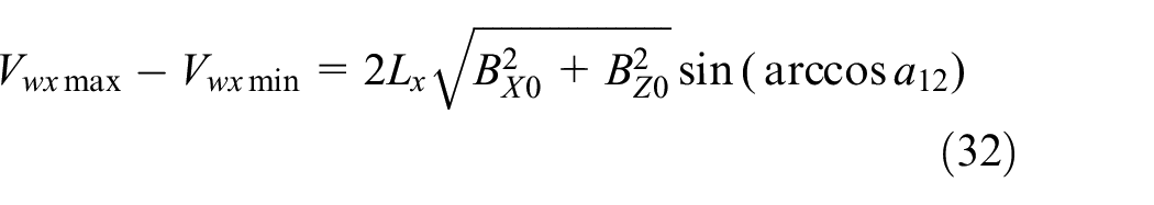
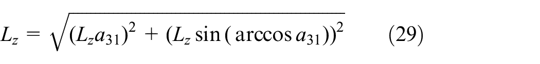
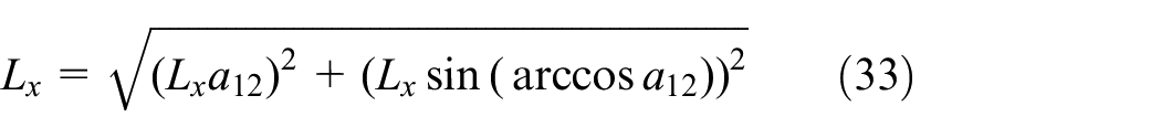
Lx can be obtained from the calculation method of equations (26) and (29), as shown in the following formula

$$L_x=\sqrt{{(L_x{a}_{12})}^2+{(L_x\sin (\arccos a_{12}))}^2}$$

(33)

Since the magnitude of geomagnetic intensity at a fixed location does not change with the direction, the equations (26), (29), and (31) are introduced into equation (1)

$${\left(\frac{V_x-V_{x90}}{L_x}\right)}^2+{\left(\frac{V_y-V_{y90}}{L_y}\right)}^2+{\left(\frac{V_z-V_{z90}}{L_z}\right)}^2=B^2$$

(34)

The zero-drift value of the three-axis of the geomagnetic sensor can be obtained by ellipsoid fitting method.

According to equation (16), the error compensation model of geomagnetic sensor can be obtained as follows

$$\left[\begin{array}{c}{B_X}_0\hfill \\ \multicolumn{1}{c}{{B_Y}_0}\\ \multicolumn{1}{c}{{B_Z}_0}\end{array}\right]={\left[\begin{array}{ccc}{a}_{11}\hfill & a_{12}\hfill & a_{13}\hfill \\ \multicolumn{1}{c}{a_{21}}& a_{22}\hfill & a_{23}\hfill \\ \multicolumn{1}{c}{a_{31}}& a_{32}\hfill & a_{33}\hfill \end{array}\right]}^{-1}\left[\begin{array}{c}{B_X}_5-P_1\hfill \\ \multicolumn{1}{c}{{B_Y}_5-P_2}\\ \multicolumn{1}{c}{{B_Z}_5-P_3}\end{array}\right]$$

(35)

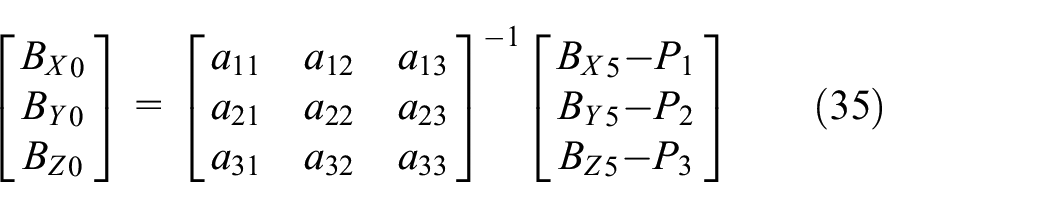
In equation (35), P1, P2, P3, a21, a31, and a12 can be solved from equations (24), (25), (27), (28), (31), and (32). Through the attitude angle experiment, the remaining six quantities can be solved, and the whole error compensation model can be solved.

Experimental verification

In order to verify the effectiveness of the compensation algorithm, we designed and manufactured a three-axis magnetic free experimental table and an aluminum table which can adjust the height. The turntable is placed on the table, and the height of the table leg is adjusted until the table level. The three-axis geomagnetic sensor is installed on the turntable, as shown in Figure 4. We selected a place in Chengdu; measured the local longitude, latitude, and altitude by theodolite; and obtained the geomagnetic parameters of the experimental site as shown in Table 1 by using the international geomagnetic reference field.

Figure 4.

Non-magnetic turntable with three-axis geomagnetic sensor.

Table 1.

Geomagnetic parameters.

Category	Size
magnetic inclination	−48.17°
magnetic declination	2.32°
magnetic field intensity	50,986.1 nT

After installation, determine the magnetic north direction and then follow the following steps for data acquisition.

1. The pitch angle is raised to 0° and 20° and the yaw angle is increased in 5° steps, so that the turntable roll axis rotates for 5 turns, and the average values of maximum and minimum output values of geomagnetic sensor Y-axis and Z-axis are recorded;

2. The pitching angle is kept at 0° and the roll angle is increased in steps of 5° to make the turntable rotate horizontally for five turns. The average values of the maximum and minimum output values of the X-axis and Z-axis of the geomagnetic sensor are recorded;

3. The output data of the sensor’s three axes are recorded when the pitch angle is 30°, the yaw angle is 45° and −45°, and the roll angle is increased in 5° steps;

4. When the pitch angle is 20° and the roll angle is 0° and the pitch angle is 30° and the roll angle is 130°, the yaw angle is increased in steps of 5° and the data of the sensor’s three axes are recorded;

The above four steps need to be carried out twice to exclude the possibility that one experiment will produce random errors.

The measurement data are summarized, and the variable L can be obtained by fitting the data from the first two steps through the least square method, and the ellipsoid as shown in Figure 5 can be obtained by using the data obtained in the last two steps into MATLAB for programming. It can be seen that the interference of the measurement environment is large. The three-axis output data distribution of the geomagnetic sensor cannot get a sphere with the center of the sphere at the origin of the coordinate. At this time, the spherical center coordinates of the ellipsoid are the zero drift values of the sensor’s three axes. The variable l obtained by fitting and the zero-drift value of the three axes of the sensor are brought into the data for calculation, and 12 parameters in the error compensation model can be obtained. After being brought into the MATLAB program for fitting, the compensated output model can be obtained, as shown in Figure 6. The output signal after compensation can be basically restored to a sphere

$$\begin{array}{c}\left[\begin{array}{c}{L}_x\hfill \\ \multicolumn{1}{c}{L_y}\\ \multicolumn{1}{c}{L_z}\end{array}\right]=\left[\begin{array}{c}0.0065\hfill \\ \multicolumn{1}{c}{0.0091}\\ \multicolumn{1}{c}{0.0089}\end{array}\right]\left[\begin{array}{c}{V}_{x90}\hfill \\ \multicolumn{1}{c}{V_{y90}}\\ \multicolumn{1}{c}{V_{z90}}\end{array}\right]=\left[\begin{array}{c}2008.7\hfill \\ \multicolumn{1}{c}{1884.4}\\ \multicolumn{1}{c}{2230.1}\end{array}\right]\hfill \\ \left[\begin{array}{ccc}{a}_{11}\hfill & a_{12}\hfill & a_{13}\hfill \\ \multicolumn{1}{c}{a_{21}}& a_{22}\hfill & a_{33}\hfill \\ \multicolumn{1}{c}{a_{31}}& a_{32}\hfill & a_{33}\hfill \end{array}\right]=\left[\begin{array}{ccc}1.7755\hfill & 0.0481\hfill & 0.0633\hfill \\ \multicolumn{1}{c}{0.0676}& -0.4627\hfill & -0.8459\hfill \\ \multicolumn{1}{c}{0.5904}& -0.7824\hfill & 0.5624\hfill \end{array}\right]\hfill \\ \left[\begin{array}{c}{P}_1\hfill \\ \multicolumn{1}{c}{P_2}\\ \multicolumn{1}{c}{P_3}\end{array}\right]=\left[\begin{array}{c}7975.7\hfill \\ \multicolumn{1}{c}{444.9103}\\ \multicolumn{1}{c}{-438.837}\end{array}\right]\hfill \end{array}$$

Figure 5.

Three-axis actual output model of geomagnetic sensor.

Figure 6.

Geomagnetic component model measured by three-axis geomagnetic sensor after correction.

After calculating and summarizing the measured data, the geomagnetic intensity error measured by the three axes of the geomagnetic sensor and the geomagnetic intensity error obtained after compensation are shown in Figure 7, in which the dotted line represents the change of geomagnetic intensity error before compensation, and the solid line represents the change of geomagnetic intensity error after compensation. It can be seen from the figure that the geomagnetic intensity error before compensation can reach 4000 nT, and the geomagnetic intensity error after compensation is reduced by 4 times compared with that before compensation.

Figure 7.

Variation of geomagnetic intensity error before and after error compensation.

Figure 8 shows the change of roll angle error before and after geomagnetic sensor output compensation, in which the dotted line represents the roll angle error before and after correction, and the solid line represents the change of roll angle error after correction. It can be seen from Figure 8 that after compensation, the roll angle error is reduced from ±6° to within ±2°.

Figure 8.

Variation of roll angle measurement error before and after compensation by geomagnetic sensor.

Conclusion

In this article, the least square method and ellipsoid fitting model are used to estimate the optimal parameters in the input–output relationship of geomagnetic sensor. The more accurate parameter values are obtained by the non-magnetic turntable experiment. Based on the analysis of the error sources in the process of geomagnetic sensor measurement, an error compensation model covering all error factors is established. All parameters in the error compensation model are removed by fitting the experimental data of attitude angle. The error compensation model is brought back to the attitude angle experiment. The experimental results show that the magnetic field strength error before compensation can reach 5000 nT, while the geomagnetic intensity error after compensation is reduced to 1000 nT, and the measurement accuracy of geomagnetic intensity is improved by 5 times; the measurement error of roll angle is reduced from ± 6° to ± 2° and the measurement accuracy is increased by 3 times, which basically meets the requirements of attitude angle measurement. Since the error compensation method discussed in this article has very low requirements for the calibration environment, it is not necessary to calibrate the three-axis geomagnetic sensor in the magnetic measurement laboratory when using this method, which effectively reduces the cost of the geomagnetic sensor in attitude measurement.