Sage Journals: Discover world-class research

Abstract

It is more practical and efficient to deploy sensors in critical areas rather than common areas to ensure indoor positioning accuracy and reduce deployment cost. This study focused on the sensor placement optimization for critical-grid coverage problem with two objectives: accuracy and cost. After reviewing some related works, this article proposed a multi-objective optimization model for critical-grid coverage problem of indoor positioning considering k-coverage problem as well as the topological rationality of sensor distribution. Then, NSGA-II algorithm was used to solve the optimizing model of sensor placement. At last, the simulation experiment and real environment validation were conducted for proposed method. The results showed that the optimized schemes obtain a lower error (1.13, 1.21 m) and a higher reduction of sensor deployment cost than the uniform deployment scheme (1.44 m). As a conclusion, the proposed method could reduce the cost of sensor deployment while ensuring the accuracy of indoor positioning for critical areas. It also provides a new direction for improving the accuracy of indoor positioning.

Keywords

Indoor positioning sensor placement optimization algorithm critical-grid coverage NSGA-II

Introduction

The applications of indoor positioning are becoming more and more important; typical examples are resource searching, tourism navigation, meeting guides, looking for the elderly and children,^1–3 and so on. These applications benefit from the technology of Wireless Sensor Networks (WSNs), mobile communication, location-aware computing,⁴ and location-based services.⁵ These services cannot be separated from the support of local position system (LPS). An LPS consists of a set of radio frequency base stations that are able to communicate with each other and locates users by measuring the received signal strength (RSS), the time difference of arrival, or the time of arrival (TOA).⁶ In LPS, each user communicates with a fixed set of base stations, and its location process is independent of that of other users, by using received signal strength indicator (RSSI) in wireless communication technologies, such as ZigBee, Wi-Fi, Bluetooth, and so on. LPS is gaining more and more popularity among the ubiquitous computing, intelligent robotics communities, and indoor positioning services in commerce.⁷

However, these different techniques of indoor positioning mentioned above have the advantages and disadvantages, and there is not yet a dominant technique to solve all problems.⁸ Thus, a number of researchers have already attempted to improve the indoor positioning algorithm to gain a higher positioning accuracy.^9–12 Those researches mostly focus on filtering sensor signals, fusing with other location signals, or improving location algorithm by compensating ranging errors to improve the accuracy of indoor positioning, while the researches on optimizing the placement of sensors are rare, especially for improving the accuracy of indoor positioning.

In addition to the accuracy of indoor positioning, there are other significant challenges, such as cost, coverage, indoor environment (obstacles), energy efficiency or lifetime, and so on. Thus, the issues of sensor distribution optimization for indoor positioning are multi-objective optimization problems. What’s more, the indoor area in which the sensors are deployed needs to be adequately distinguished as “critical areas” and “common areas” in many indoor applications. For example, in a railway station or airport, critical areas are the “hot spots,” such as elevator entrance, boarding gate, toilet and service center, and common areas are the waiting area, excluding the critical areas. Critical areas and common areas have different positioning needs and should be differentiated.¹³ It is more practical and efficient to deploy sensors in critical areas rather than common areas to ensure positioning accuracy and reduce deployment cost.

Therefore, this study focused on the sensor placement optimization for critical-grid coverage problem¹⁴ with two objectives of accuracy and cost. The contributions of this article include the following:

Review of the state-of-the art sensor placement optimization focusing on indoor positioning;

Proposal of the geometry model of sensor coverage for critical-grid coverage problem of indoor positioning;

Proposal of optimizing model of sensor placement for critical-grid coverage problem of indoor positioning and its computing method;

Numerous simulations, analysis, and real environment example for the validation of the proposed method.

The article is outlined as follows. The “Related works” section reviews some related works. The section “Computing model for critical-grid coverage” proposes the computing model of sensor coverage for critical-grid coverage problem of indoor positioning. The section “Optimizing model of sensor placement” introduces optimizing model of sensor placement for critical-grid coverage problem of indoor positioning and its computing method. The “Experiment and validation” section presents simulation results and analyses of experiments and real environment validation for proposed method. The “Conclusion” section concludes the article and presents future work.

Related works

The emerging WSNs technology provides an inexpensive and powerful means to monitor physical environments.^5–7 In a typical sensor network application, sensors are to be placed (or deployed) so as to monitor a region or a set of points. Sensor deployment has corresponding methods or algorithms, which can be summarized as follows: deterministic sensor deployment and nondeterministic sensor deployment.¹⁵ The difference of the two methods depends on whether the environment permits location selection for sensor deployment. Early researches were mainly focused on theoretical exploration and mathematical expression of models or algorithms for sensor deployment, and sensing coverage and connectivity of the WSNs were of great concern.^16,17

Considering the coverage of critical area, research can be summarized into two categories: area coverage and target or point coverage.¹⁴ On the problem of area coverage, the sensing range of the deployed sensors should cover a specific given area (critical area), whereas, in regard to the target or point coverage, as the name suggests, a set of specific given targets or points should be monitored by sensors. Since the space of sensor placement is usually divided into square grids,^13,14,18 the goal is to construct a full coverage of critical square grids with the minimum number of sensors on square grids, termed critical-square-grid coverage. Furthermore, most of these coverage problems are defined as NP-hard optimization problems.^13,19 To obtain optimal solutions of sensor placement, many researchers have to turn to the heuristic algorithms, such as genetic algorithm,^20,21 simulated annealing,²² monkey algorithm,²³ ant colony algorithm,²⁴ and particle swarm optimization.²⁵ However, these studies do not emphasize critical area coverage problems of sensor placement for indoor positioning.

The critical area coverage problems of sensor placement for indoor positioning are significant for decision making in some situations,²⁶ such as fire rescue, medical monitoring, indoor navigation, and so on. In previous studies, there are a few studies on optimization of sensor placement for indoor positioning in this field. Vlasenko et al.²⁷ proposed a methodology of optimizing sensor placement for indoor localization in the platform of the Smart-Condo, and the frequently visited areas of the living space covered by a number of sensors were the optimization objective. Berka et al.²⁸ proposed a method to optimize the number of sensor nodes near decision points for intermodal navigation of blind pedestrians. In Domingo-Perez’s²⁹ sutdy, the number of sensors, accuracy and coverage were taken into account for optimizing the sensor deployment in the region of interest. However, researches on sensor placement optimization of critical-grid coverage problem of indoor positioning have not been reported yet.

Concerning the multi-objective optimization algorithms, the NSGA-II was the most used algorithm in previous studies. Chen et al.³⁰ proposed a solution based on NSGA-II to make fuller use of the whole sensor nodes and further increase the network lifetime. Yang et al.³¹ presented the optimizations of a space-based reconfigurable sensor network under hard constraints by employing NSGA-II to find multi-criteria solutions in the sense of Pareto optimality. Syarif et al.³² conducted a study based on NSGA-II for achieving coverage and connectivity as two fundamental issues in WSNs, and introduced Network Simulator, NS-2, used for network simulation to verify the performance of optimized solution. Le Berre et al.³³ proposed a modified NSGA-II of bi-objective sensor placement with the minimization of the number of deployed sensors and the minimization of the tracking constraints violations, under the coverage constraints. In Hasson and Khudhair’s³⁴ study, NSGA-II is used recently as a tool to obtain the best trade-off between network coverage and connectivity as two competing objectives. Harizan and Kuila³⁵ proposed a novel NSGA-II with modified dominance to solve the multi-objective coverage and connectivity problem. In some others’ studies, NSGA-II algorithm was used for comparison with other algorithms for multi-objective optimization of sensor coverage problems.^36–38 However, the validation for proposed method in most previous studies is by numerical simulations. There are few real case studies for the method validation or evaluation.

Due to the unique computing characteristics of indoor positioning, the sensor coverage is different from that mentioned above. In indoor positioning application, the sensor coverage usually involves the problem of multiple sensors coverage, which means that each target in the sensing area needs to be covered by at least k (k ≥ 3) different working sensors,⁸ known as k-coverage problems.³⁹ This might increase the complexity of sensor placement optimization in geometrical representation, topology structure, and computation. The topological rationality of sensor distribution should be considered in the optimization.

To sum up, from early works of literature, most of published works in sensor placement optimization use the NSGA-II to achieve the multi-objective optimization (i.e. coverage, connectivity, energy efficiency, number of sensors, etc.). Very few works talk about the critical-grid coverage problem of indoor positioning in this field. Furthermore, from practical point of view, real case study in indoor positioning by using the optimized sensor deployment may also be needed, because the real environment is usually different from the ideal conditions in numerical simulations. However, this is very important for the practical application of the algorithm. In this article, some crucial topics of the sensor placement optimization are stated as follows:

The multi-objective optimization using NSGA-II for the critical-grid coverage problem;

The k-coverage problem as well as the topological rationality of sensor distribution;

The real environment case study by using the optimized sensor deployment in indoor position.

Computing model for critical-grid coverage

Geometry model of sensor coverage

The given space of sensor deployment is decomposed into small contiguous regular grids in previous studies.^{13,14,18,40,41} This concept is also adopted in this article. Since the three-dimensional (3-D) potential coverage space is complex and challenging, in order to facilitate the discussion of sensor deployment, two-dimensional (2-D) potential space is discussed in this study. The 2-D potential space is divided into small grids, and each grid is characterized by a length a and a width b (a and b are less than R, the effective sensing range of a sensor). The center point of each grid is the potential placement of a sensor. Only one sensor can be deployed in a grid. In this article, the grid is considered to be covered when the center point falls within the sensing range. The model is depicted in Figure 1. In this case, b < a < R, and nine grids are covered in the sensing range.

Figure 1.

Grid division and sensor coverage model.

Sensor coverage problems can be divided in the ONE-coverage problem or the k-coverage problem.¹⁴ The k-coverage of the targets indicates that each target node must be covered by at least k sensor nodes.³⁹ How many sensor nodes are needed depends on the specific issues and requirements of the applications. The higher k is, the more expensive the WSN costs, but the more stable the WSN is. Even after failure of k− 1 sensor nodes, the target will still remain covered. However, in some applications, k must be greater than 3. In that case, the two-coverage is a failure. The concept of the k-coverage model (i.e. k = 2, 3, 4) can be seen in Figure 2. In the indoor positioning application, how many sensors are needed depends on the method used for positioning calculation.⁸

Figure 2.

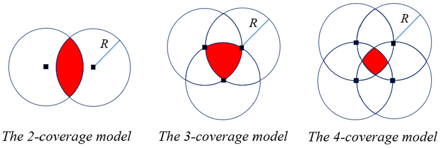
The k-coverage model (i.e. k = 2, 3, 4).

Method of indoor positioning calculation

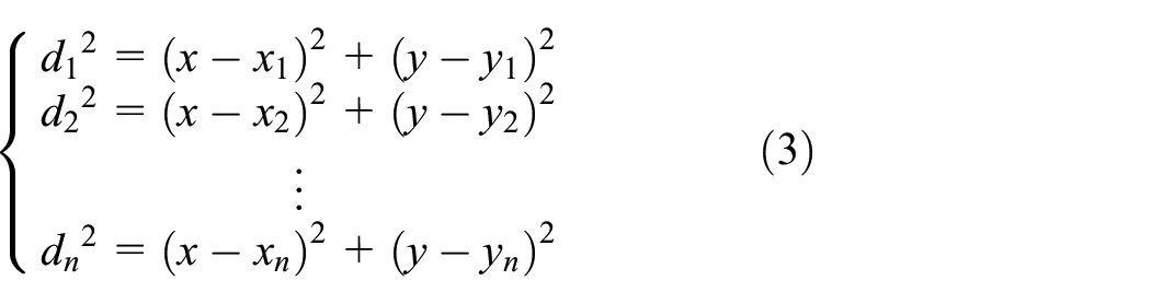
Recent approaches of indoor positioning are generally based on distance measurement.¹¹ The indoor positioning algorithm of distance measurement is to measure the distance between the target node and its anchor node (sensor), and then calculate the coordinates of the target node according to the geometric principles. The most commonly used indoor positioning algorithms of distance measurement are trilateration, time of flight, and maximum likelihood estimation methods,¹¹ and the calculation of the coordinates of the target node needs the help of at least 3 anchor nodes (three-coverage requirement), for example, by the trilateration algorithm. The principle of trilateration is shown in Figure 3(a). The coordinates of three points are known as (x₁, y₁), (x₂, y₂), (x₃, y₃) and their distances from target node are d₁, d₂, and d₃, respectively. Assuming that the coordinates of target node are (x, y), the following equation exists

{\begin{matrix} d_{1} = \sqrt{{(x - x_{1})}^{2} + {(y - y_{1})}^{2}} \\ d_{2} = \sqrt{{(x - x_{2})}^{2} + {(y - y_{2})}^{2}} \\ d_{3} = \sqrt{{(x - x_{3})}^{2} + {(y - y_{3})}^{2}} \end{matrix}

(1)

Figure 3.

(a) The principle of trilateration and (b) the principle of maximum likelihood estimation.

The coordinates of target node to be measured can be obtained from the above formula as follows

\begin{array}{l} [\begin{matrix} x \\ y \end{matrix}] = {[\begin{matrix} 2 (x_{1} - x_{3}) & 2 (y_{1} - y_{3}) \\ 2 (x_{2} - x_{3}) & 2 (y_{2} - y_{3}) \end{matrix}]}^{- 1} \\ [\begin{matrix} {x_{1}}^{2} - {x_{3}}^{2} + {y_{1}}^{2} - {y_{3}}^{2} + {d_{3}}^{2} - {d_{1}}^{2} \\ {x_{2}}^{2} - {x_{3}}^{2} + {y_{2}}^{2} - {y_{3}}^{2} + {d_{3}}^{2} - {d_{2}}^{2} \end{matrix}] \end{array}

(2)

Time of flight or TOA exploits the signal propagation time to calculate the distance between the anchor node and target node. The time of flight value multiplied by the speed of light c = 3×10⁸ m/s provides the physical distance between the anchor node and target node. Similar to principle of trilateration, by using three different anchor nodes to estimate the distances between the anchor node and target node, the coordinates of target node can be obtained.

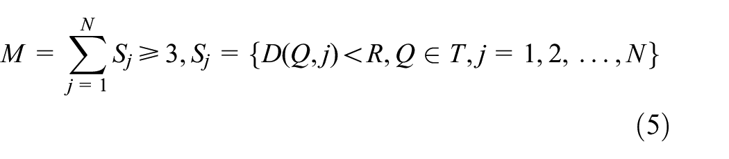
Maximum likelihood estimation requires k-coverage of target node, and k is more than three. With the coordinates of k sensors and the distances between each sensor and target, k equations can be established. The principle is shown in Figure 3(b): N anchor node coordinates are (x₁, y₁), (x₂, y₂), (x₃, y₃), …, (x_n, y_n) and their distances from point E (target node) to be measured are d₁, d₂, d₃, and (…), d_n. Assuming that the coordinates of E is (x, y), the following equations exist

{\begin{matrix} {d_{1}}^{2} = {(x - x_{1})}^{2} + {(y - y_{1})}^{2} \\ {d_{2}}^{2} = {(x - x_{2})}^{2} + {(y - y_{2})}^{2} \\ ⋮ \\ {d_{n}}^{2} = {(x - x_{n})}^{2} + {(y - y_{n})}^{2} \end{matrix}

(3)

The method of standard minimum mean square error estimation is used in the maximum likelihood estimation to obtain coordinates of the target node.

Through the analysis of the above algorithms, some conclusions can be drawn. First, the indoor positioning by using those algorithms is a typical k-coverage problem. Second, distance estimation is one of the important factors of positioning accuracy. Furthermore, in calculating the distance from the target node to the sensor node, the received signal must be stronger than the disturbance signal amplitude of the sensor itself, otherwise the distance estimation will be inaccurate.^9,10 Thus, the distance estimation between the sensor and target may be the direction to improve the indoor positioning accuracy.

According to the principle of indoor positioning algorithm based on distance measurement, the higher the accuracy of the distance between sensor and target is, the more accurate the coordinate calculation of the target node is. As a result, a higher positioning accuracy will be obtained. Therefore, theoretically, ensuring the target node within the sensor range can improve the accuracy of distance between the target node and the anchor node, which is important to ensure the accuracy of indoor positioning.

Geometry model of critical-grid coverage

In indoor positioning application, the difference of definitions for critical grids (hot spots or interest points) has been obviously recognized due to the different objectives, users, and other facts of the application.¹⁴ However, the decision points are the most critical grids in indoor positioning, since the navigation instruction is needed because of multiple routes such as entrances or exits to buildings, corridor crossing or road intersections, stairs or lifts, toilet, and other interest points.^13,27 Thus, this study assumes that the critical grids are those decision points, and n decision points (critical grids) are manually designated according to the rule that whether these decision points can help people make decisions. These points need to ensure their positioning accuracy, or the highest positioning accuracy in the whole indoor region.

Figure 4(a) is an example of the critical areas of a concept indoor environment, and Figure 4(b) shows the critical-grid coverage model derived from Figure 4(a). Exits, road intersections, lifts, and toilet are considered as the decision points. In this example, the map of indoor environment is converted to the sensor coverage model described above, and a critical grid is covered by three sensors.

Figure 4.

Concept of critical-grid coverage model for indoor positioning: (a) Critical areas of a concept indoor environment and (b) critical-grid coverage model.

Optimizing model of sensor placement

Description of problem

According to the geometry model of critical-grid coverage for indoor positioning, the optimization problem initially can be descripted as maximizing the critical-grid coverage, and minimizing the number of sensors. Assuming that the trilateration method is used in the indoor positioning, to ensure the positioning accuracy of critical grids, the target node should be k-covered, and k ≥ 3. In terms of topological rationality of sensor distribution, some restrictions will be considered in the optimization.

Thus, the optimization problem in this study can be descripted as follows: the 2-D plane space is divided into a number of grids, among which there are a number of critical grids. Assuming that only one sensor can be deployed in each grid, and no sensor can be deployed in the adjacent grids of the grid with a deployed sensor, this is the topological rationality of sensor distribution in this study. Figure 5 is an example for the topological restriction of sensor distribution. When a sensor is deployed in a grid, the eight adjacent grids of the grid prohibit the deployment of sensors as shown in Figure 5. This is to make the sensor deployment as decentralized as possible to adapt to the triangulation algorithm.

Figure 5.

The topological restriction of sensor distribution.

To represent the topological rationality of sensor distribution, the topological restriction need to be tested and verified. Thus, a case study in the real indoor environment is required by evaluating the positioning accuracy for the optimized scheme of sensor deployment, and then comparing the proposed method to traditional method. By this way, the advance of the proposed method can be clearly observed.

Due to that the different schemes of sensor deployment have different coverage for critical grids (i.e. distance between the sensor and target, topological structure of sensors and targets), which results in different positioning accuracy and deployment cost. How to deploy sensors to achieve the highest coverage (accuracy) and the lowest cost for critical grids is the focus of this article. The mathematical expression of the optimization model will be introduced in the next section.

Expression of optimization model

The critical-grid coverage problem is converted to the question, how many target nodes are located in the effective distance of a sensor? Meanwhile, the number of sensors for each target node must be not less than three within the effective sensing range. The first objective function of optimization model is as follows:

Suppose i is the i-th sensor, J is the total number of sensors, S is the set of target nodes, P is a subset of S, and R is the maximum effective distance from a sensor. Assuming that a target node is located in the sensing range of a sensor, the sensor is called the effective sensor of the target node. We denote with T₁ the number of target nodes within the effective distance of each sensor. Therefore, the objective function, maximum target nodes per effective sensor is expressed as follows

\begin{matrix} Maximize : T 1 = \frac{\sum_{i}^{J} N_{i}}{J} \\ N_{i} = {D (P, i) < R, P \in S, i = 1, 2, \dots, J} \end{matrix}

(4)

where N_i is the number of target node within the range of the i-th sensor, and D (P, i) represents the distance between the i-th sensor and target node in P set. Each sensor has a corresponding P set, in which each target node in P set must satisfy the condition that the distance between the sensor and target node should be less than R. For a given sensor placement scheme, the P set for each sensor can be generated by the following steps:

Distance calculation: Calculating the distance between each sensor and all target nodes.

Effective sensor checking: If the distance is less than R, the sensor is the effective sensor of the target node, and put this target node in the P set of the sensor.

Traversal circulation: Traversing all sensors in the given sensors set for distance calculation and effective sensor checking, all P sets have been generated for each sensor.

Due to the three-coverage requirement of indoor positioning, the constraint is considered as follows:

Assuming that the number of target nodes is N and j is the j-th target node, the number of sensors within the distance R for each target node (S_j) is greater than or equal to 3, and its mathematical expression is as follows

M = \sum_{j = 1}^{N} S_{j} \geq 3, S_{j} = {D (Q, j) < R, Q \in T, j = 1, 2, \dots, N}

(5)

where M is the number of sensors for each target node. D (Q, j) represents the distance between the i-th target and the sensor in Q set. Q is a subset in set of all target nodes (T), and the method for calculating Q set is similar to P set in equation (4).

For the second objective function, assuming that the cost of each sensor is Y and the number of sensor is J, the expression of minimum total cost of deployment scheme is T₂. The second objective function of optimization model can be demonstrated as

Minimize : T_{2} = Y \times J

(6)

Model solving method

As mentioned in the literature review, NSGA-II is used recently as a tool to solve many multi-objective optimization problems in WSNs. Deb et al.⁴² propose an improved version of NSGA-I, named NSGA-II. The NSGA-II procedure starts by building a population of individuals. Next, the candidate solutions are sorted and ranked in fronts according to a non-dominance rule. Then, it applies the evolutionary operators, namely, the crossover and the mutation to find a new population of off-springs. The crowding distance determines how far each solution is from others in the same front, and it aimed at keeping the diversity among the solutions. This guarantees the diversity of the population and improves the exploration of the fitness landscape.³⁵

In this study, NSGA-II is used to solve the multi-objective optimization problem. In the GA, the decision variables are coded into chromosomes, and the fitness value (objective function value) of chromosomes is calculated.³² Thus, the 2-D plane grids are transformed into gene chain of a chromosome through the grid ID, as shown in Figure 6. Suppose the 2-D plane is divided into K grids, and they are indexed by grid ID starting from 1. The binary coding is used to transform the decision variables into a chromosome. Since the sensor has K alternate locations, each scheme of sensor deployment can be represented by K binary digits in a chromosome. When the value of the gene is 0, there is no sensor in the position; when the value of the gene is 1, the sensor is present in that explicit position recognized by grid ID. For simplicity, the coordinates of a grid center stand for the grid. They can be figured out in the 2-D coordinates. The grid ID links the gene chain of a chromosome, as well as the coordinates of the grid center in the 2-D coordinates. By this way, the connection between chromosome and 2-D grid is established.

Figure 6.

A chromosome representation for WSNs.

The cost of sensor deployment scheme, as the second objective, can be easily obtained by summarizing the number of gene with value of 1, while the calculation of the first objective function may not be uncomplicated. First of all, the chromosome needs convert to the location (coordinates) in the 2-D plane by the grid ID. Second, the calculation of distance between each sensor and each target node should be done. Third, the value of the first objective function and its constraint can be obtained. What’s more, the topological restriction of sensor distribution should be considered beforehand in the generation of father chromosomes and off-springs.

The steps of NSGA-II algorithm for sensor placement optimization are as follows:

Step 1: Random generation of original population with size of P. Each of these individuals represents a set of sensor arrangements, and each position represents a gene. Set t = 1.

Step 2: Updating each individual to satisfy the constraints. First, no sensor is deployed in its adjacent grids in the 2-D plane. To do this, examine all grids, if the value of gene is 1, find the site of the grid in the 2-D plane by the ID of the gene chain, and then find its adjacent grids (eight grids) and their IDs of the gene chain. If the value among the eight genes is 1, change it to 0. Second, according to formula (5), the number of effective sensors for each target node must be not less than three. To satisfy this, each target node will be checked. If its effective sensors is less than three, additional sensors should be added. Accordingly, the value of the gene in right position of gene chain is modified from 0 to 1. Figure 7 is an example for updating each individual to satisfy the constraints.

Step 3: Evaluation of objective function T1 and T2 of each individual according to formulas (4) and (6). In this case, each scheme of sensor deployment corresponds to two objective function values.

Step 4: Non-dominant sorting for each individual. According to the value of objective functions, the population is divided into different non-inferior layers by non-dominant sorting. The non-dominant solutions (non-inferior layers) will be reserved to an elite set with size of P by the crowded comparison operator⁴² and updated for each iteration.

Step 5: Judgment of termination conditions. If the termination condition is reached (e.g. t > maximum generation), the iteration will stop; otherwise, go to Step 6. Maximum generation is one of the parameters commonly used in termination conditions of NSGA-II algorithms. As a known input parameter of the algorithm, it is specified by the user, for example, 100, 500, and so on.

Step 6: New population generation. First, establishing the optimization pool. Two individuals are selected randomly from parent population (elite set), and according to the non-inferior layers, the better one is chosen and put into the optimization pool; Second, generating child population through crossover and mutation operations. Crossover operations—two individuals are randomly selected from the optimization pool and a portion of the genes in the two individuals are randomly exchanged. Mutation operations—an individual is randomly selected from the pool of preferences, and a random exchange exchanges a portion of the genes in the individual. The method used in this study is similar to Li et al.²¹ Finally, combining the parent population and child population to generate a new population, t = t + 1, and go back to Step 2.

Figure 7.

An example for updating each individual to satisfy the constraints.

Experiment and validation

Introduction of optimization experiment

The sensors selected in this experiment were iBeacons, as the anchor nodes. iBeacon technology was launched by Apple in 2014.⁴³ Based on Bluetooth 4.0 technology, iBeacon stands out in the crowd of positioning sensors because of its low power consumption, fast response, good performance, and low price. Moreover, even the cheapest smart phones embeds Bluetooth module, which makes iBeacon be widely used and deployed.

With the change of the distance between the smart phone and the iBeacon node, the change of the received signal intensity value (RSSI) is observed, which provides a theoretical basis for the maximum effective distance R from the sensor. Eight groups of data were measured in the experiment, as shown in Figure 8. It can be found from the graph that when the distance in the range from 0 to 3 m, the value of RSSI decreases sharply. When the distance is more than 3 m, the value of RSSI tends to change smoothly with the increase of the distance. To guarantee the positioning accuracy, the maximum effective distance R from the iBeacon was 3 m, and this was consistent with Ng⁴⁴ study.

Figure 8.

Attenuation characteristic map of iBeacon signal.

In this experiment, the underground parking lot of a university was selected as the optimization placement of iBeacon, and the parking space was transformed into 2-D coordinate system, as shown in Figure 9. According to the parking environment, some important areas and interest points were designated as the target nodes, a total of 24 target nodes. These nodes were evenly uniform distributed over the main road of the indoor parking lot for the purpose of indoor navigation application. The potential deploy space of iBeacon was within the range of red polygon as shown in Figure 9. The space outside of the red polygon was supposed to be not critical in the indoor parking lot. In the red polygon, the potential deploy space was divided into 1-m-square grids, with a total of 495 grids.

Figure 9.

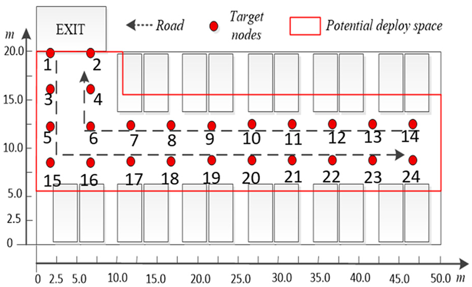
Distribution map of target nodes in an underground parking lot.

Validation method

In order to validate the proposed method of sensor placement optimization for critical-grid coverage problem, it was compared with the traditional deployment method. Traditional deployment methods include uniform deployment and staggered triangular grid deployment. In this article, uniform deployment method was selected as comparison purpose (hereinafter referred to as the control scheme). The uniform deployment scheme is that the distance between two deployed iBeacon nodes is controlled at a fixed distance. In this article, the distance is 3 m, which is consistent with the maximum effective distance R of iBeacon.

In terms of quantitative indicators for evaluating sensor deployment schemes, this article evaluated them from two perspectives:

The two indicators of deployment scheme were the number of target nodes within the effective distance (R) of each sensor (T₁) and the cost (T₂);

Real environment comparison: comparing the average positioning error of the same observation points of the two schemes—the optimized scheme and the control scheme.

Results and discussion

Simulation results

In the parameter setting of the NSGA-II algorithm, the population size is 100, the crossover rate is 0.5, and the mutation rate is 0.3. Different evolutionary generations are used as termination conditions. The termination conditions are 100, 200, 500, 1000, 5000, and 10,000 generations, respectively. The experiment ran on a general computing server, whose processor was Intel (R) Xeon (R) CPU E3-1535M, 2.9 GHz with 16 GB of memory.

The computation time and objective function values under different generations are shown in Table 1. As can be seen from the table, with the increase of generation, the target T₂ (cost) decreases gradually and the computation time multiplied increase within acceptable range, while the target T₁ is viewed an increase trend, which means maximizing utilization of each sensor for these 24 target nodes. In the worst case, with the increase of T₂, T₁ remains unchanged or decreases. This indicates that the increased number of sensors is not fully utilized. Therefore, this shows the effectiveness of the optimization method.

Table 1.

Operational time and objective function values of the algorithm under different generation compared with control scheme.

Generation	100	200	500	1000	5000	10,000	Control scheme
Computation time (s)	15.1	25.1	62.0	149.9	752.0	1412.7	–
Target T₁	1.69	1.74	1.77	1.81	1.76	1.79	1.86
Target T₂	2600	2480	2440	2320	2200	2120	3040

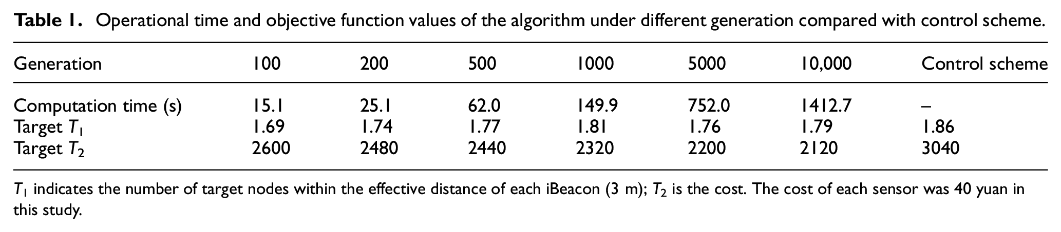
T ₁ indicates the number of target nodes within the effective distance of each iBeacon (3 m); T₂ is the cost. The cost of each sensor was 40 yuan in this study.

The T₁ of the control scheme in Table 1 is slightly higher than that of all the optimized deployment schemes, but its deployment cost (T₂) is relatively high. In general, the deployment scheme can be seen as a cost-effective scheme when T₂ is low and T₁ is high. The reason for the higher values of T₁ in control scheme might be that it spends more money to increase the sensors, and the number of target nodes is also 24. With the increase of sensors, average number of sensor might increase for each target node, and then increase the value of T₁. Nevertheless, the control scheme has certain advantages in general, but the optimized method may lead to cost-effective schemes in specific situations. It should be highlighted that, according to Table 1, after 10,000 iterations of the NSGA-II algorithm, the cost T₂ (i.e. the number of nodes) is reduced by about 30% with respect to the control scheme, while the coverage (T₁) is reduced by 3.8%. This seemingly suggests that strong saving may be achieved without a significant coverage reduction.

Contrast experiment under real environment

In order to do further verification and evaluation of the proposed method, a LPS was built. The LPS was composed of a server and iBeacons deployed according to an optimized scheme and a control scheme. The server is a Dell computer, with an Intel CORE i5 processor, and 8 GB memory. Each iBeacon was set to a 10 Hz sample rate with 0 dBm transmit power. The mobile platform is a smart phone of Huawei with an Android 6.0 operation system. The trilateration method is used in the experiment to calculate the position of an unknown node. Considering the cost of LPS in real environment, this article chooses the optimized schemes with generation number of 100 (Scheme A with 65 sensors), 500 (Scheme B with 61 sensors) from Table 1 and the control scheme, as shown in Figure 10. In control scheme, the number of sensors was 76.

Figure 10.

Spatial distribution map of target nodes, optimized scheme, and control scheme under different generations.

Then, each point of 24 target nodes was tested three times. The positioning errors of these points are observed and the average errors are calculated to evaluate different schemes of sensor deployment. The error formula adopted in this experiment is as follows

E = \sqrt{{(x_{p} - x_{p 0})}^{2} + {(y_{p} - y_{p 0})}^{2}}

(7)

where E represents error, (x_p, y_p) represents the location coordinates of the target node measured by LPS, and (x_p₀, y_p₀) represents the real coordinates of the target node.

To describe the Error distribution of each target node in Scheme A, Scheme B, and Scheme C, the Geometrical Dilution of Precision (GDOP) is given in Figure 11. It can be seen that none of the schemes achieves minimum error for all target nodes. This may be related to the spatial location of the target nodes and anchor nodes. Different schemes have different spatial distribution of sensors. Each scheme has its advantages.

Figure 11.

Geometrical Dilution of Precision of each target node in optimized schemes (100-generation, 500-generation) and control scheme.

From GDOP in Figure 11 and the spatial distribution of iBeacon nodes in Figure 10, some rules or characteristics of sensor placement can be found. First of all, the closer the distance between the anchor nodes and the target node is, the smaller the positioning error of the node is. For example, the target node ID of 8 in Scheme B, and target node ID of 19 in Scheme A. Second, for some target nodes with large positioning errors, the spatial placement of sensors is characterized by the fact that the target nodes are not completely surrounded by the anchor nodes, or that the target nodes are outside the triangle surrounded by three anchor nodes. The examples are Target Node 4 in Scheme B, Target Node 9 in Scheme C, and Target Node 12 in Scheme A. Third, for some of target nodes with similar positioning errors in the three schemes, the spatial layout of sensors is characterized by the fact that in the optimized scheme, the distance between the anchor nodes and the target node is closer than that in the control scheme, and the target nodes are not completely surrounded by the anchor nodes, such as the target node IDs of 7, 10, and 24. This indicates that the topological structure of sensors and targets can significantly affect the performance of particular positioning algorithm, which is also mentioned in Bishop et al.’s⁴⁵ research.

Table 2 shows the average errors of 24 target nodes under 100 generations (Scheme A), 500 generations (Scheme B), and control scheme (Scheme C). The average errors were more than 1 m for all of the three schemes, since iBeacon is not good at precise positioning and is suitable for proximity positioning.⁴⁶ The average error of Scheme B was 1.13 m, similar to Chen et al.’s⁴⁷ in which the average error was 1.11 m. The maximum errors of the two Scheme were 1.89 and 2.39 m, respectively, which was smaller than 2.77 m in Chen et al.’s study.⁴⁷ A smaller error of optimized scheme can be observed compared with control scheme. This indicates that the optimization of sensor placement for critical-grid coverage can reduce the error of indoor positioning. Furthermore, it provides a new direction for improving the accuracy of indoor positioning, besides the methods of signal filtering, multi-signal fusion, and localization algorithm improvement.

Table 2.

Average error and maximum error of optimized 100-generation, 500-generation, and control schemes.

Target Node ID	Error of Scheme A	Error of Scheme B	Error of control scheme
Average (m)	1.21	1.13	1.44
Maximum (m)	1.89	2.39	2.58
Standard deviation	0.28	0.29	0.32

In Table 2, it shows that with the increase of optimization generation, the average error of 24 target nodes may decrease, while the average error of the control scheme is the largest one. The standard deviation for optimized schemes is slightly smaller than the control scheme. This implies that the optimization method for critical areas is better than the traditional uniform sensor deployment in this study. The reason might be that the locations of iBeacon nodes were around the target nodes (at least three anchor nodes surround one target node) in the optimized schemes, while in the control scheme, sensors were evenly distributed and could not completely surround all target nodes, especially for such cases showed in Figure 12. The distance between target node to anchor node of C is larger than 3 m. This would increase the error of measured distance due to the attenuation characteristic of iBeacon, which was discussed in the “Introduction of optimization experiment” section. This might be the reason why average error of target node ID from 1 to 14 was a little higher than that of target node ID from 15 to 24 in Figure 8.

Figure 12.

An example of target node and anchor nodes in the control scheme.

By analyzing Figure 10 and Table 2, the NSGA-II optimization method led to a reduction of sensors for optimized schemes compared to the control scheme. For Scheme A, the reduction is about 15% (number of sensors from 76 to 65), and for Scheme B, the reduction is about 20% (number of sensors from 76 to 61). At meantime, about 21.5% accuracy improvement was also obtained due to average error from 1.44 to 1.13 m comparing Scheme B to the control scheme. Thus, it can be stated that the proposed optimization method may lead a 21.5% accuracy improvement, with a cost reduction of about 20%.

In this study, the positioning error of some nodes in the optimized scheme is higher than that in the uniform deployment, which indicates that the optimized scheme is not globally optimal, or the optimization objective functions need further improvement in the future study. The sensitivity studies for parameters and the effect of scalarization on the optimization problem, discussed by Soman et al.,⁴⁸ have not been conducted in this study, since the focus of this article is on sensor placement optimization for solving the critical-grid coverage problem. Sensor deployment in environments containing obstacles also attracted a lot of attention by WSN researchers.⁴⁹ Our future studies may focus on sensor placement optimization for critical-grid coverage problem considering obstacles, parameter sensitivity, and scalarization effects.

Conclusion

There is a great demand for indoor positioning. The indoor positioning accuracy of critical areas and interest points is becoming higher and higher. Starting from the related work of sensor optimization, the computing model for critical-grid coverage, and the optimizing model of sensor placement were introduced. NSGA-II algorithm is used to optimize the placement of iBeacon nodes. In order to verify the proposed method, a real example of the underground parking lot of a university was given, and the simulation and the comparative analysis were conducted. The results showed that the optimized schemes had a better accuracy than the control scheme in general within a relatively short period of computing time. This might be due to the fact that the optimized schemes have a more reasonable sensor-target geometry, which is more suitable for the indoor positioning algorithm of distance measurement, and thus the positioning error of optimized schemes was lower than the uniform deployment scheme. As a conclusion, the proposed method could reduce the sensor deployment cost while ensuring the positioning accuracy of indoor critical areas. In addition to the other common techniques, such as signal filtering, multi-signal fusion, localization algorithm improvement, and so on, this work provides a new direction for improving the accuracy of indoor positioning.

In future, further research will be needed, such as (1) the complex indoor environment, such as the obstacles which will block sensor signal; (2) the spatial resolution (scalarization) which may increase the computation cost; and (3) inherent adaptability of the different methods of indoor positioning calculation (algorithms), such as maximum likelihood estimation, centroid algorithm and fingerprint algorithm, and different topological structures of sensor deployment.

Footnotes

Handling Editor: Lyudmila Mihaylova

Declaration of conflicting interests

The author(s) declared no potential conflicts of interest with respect to the research, authorship, and/or publication of this article.

Funding

The author(s) disclosed receipt of the following financial support for the research, authorship, and/or publication of this article: This study was funded by the Basic Research Plan for Public Welfare of Zhejiang Province (LGG21A010001), the Provincial Key Research and Development Program of Zhejiang (2018C01016), and the Scientific Research Project of Zhejiang Education Department (Y201942160).

ORCID iD

Zhe Liu

References

Zhao

Wang

, et al. Study on key technologies of Location-Based Service (LBS) for forest resource management. Njas-wagen J Life Sc 2012; 10: 292–300.

Tiru

Kuusik

Lamp

, et al. LBS in marketing and tourism management: measuring destination loyalty with mobile positioning data. J Locat Based Serv 2010; 4: 120–140.

Santoso

Redmond

SJ.

Indoor location-aware medical systems for smart homecare and telehealth monitoring: state-of-the-art. Physiol Meas 2015; 36: R53–R87.

Hazas

Scott

Krumm

Location-aware computing comes of age. Comput 2004; 37: 95–97.

Mountain

Raper

Positioning techniques for location-based services (LBS): characteristics and limitations of proposed solutions. Aslib Proc 2001; 53: 404–412.

Werb

Lanzl

Designing a positioning system for finding things and people indoors. IEEE Spectrum 1998; 35: 71–78.

Shimosaka

Saisho

Sunakawa

, et al. ZigBee based wireless indoor localization with sensor placement optimization towards practical home sensing. Adv Robotics 2016; 30: 1–11.

Zafari

Gkelias

Leung

A survey of indoor localization systems and technologies. IEEE Commun Surv Tut 2017; 21: 1–26.

Tseng

Yen

JS.

Enhanced Gaussian mixture model of RSSI purification for indoor positioning. J Syst Architect 2017; 81: 1–6.

10.

Wang

ZX.

Indoor location algorithm based on the measurement of the received signal strength. Front Electr Electron Eng China 2006; 1: 48–52.

11.

Czapiewska

New indoor positioning algorithm for distance measurements. In: Proceedings of the IEEE international conference on telecommunications & signal processing, Barcelona, 5–7 July 2017, pp. 225–228. New York: IEEE.

12.

Han

Jiang

Kong

, et al. Indoor localization within multi-story buildings using MAC and RSSI fingerprint vectors. Sensors 2019; 19: 2433.

13.

Liu

Tsai

MJ.

The critical-square-grid coverage problem in wireless sensor networks is NP-Complete. Comput Netw 2011; 55: 2209–2220.

14.

Rebai

Berre

Hnaien

, et al. A branch and bound algorithm for the critical grid coverage problem in wireless sensor networks. Int J Distrib Sens N 2014; 1: 769658.

15.

Sahni

Algorithms for wireless sensor networks. Int J Distrib Sens N 2010; 1: 35–56.

16.

Wang

Xing

Zhang

, et al. Integrated coverage and connectivity configuration in wireless sensor networks. In: Proceedings of the ACM conference on embedded networked sensor systems, Los Angeles, CA, 5–7 November 2003, pp. 28–39. New York: ACM.

17.

Zhang

Hou

JC.

Maintaining sensing coverage and connectivity in large sensor networks. Ad Hoc Sens Wirel Ne 2004; 1: 1–15.

18.

Chakrabarty

Iyengar

, et al. Grid coverage for surveillance and target location in distributed sensor networks. IEEE T Comput 2003; 51: 1448–1453.

19.

Liu

Tsai

MJ.

Constructing a wireless sensor network to fully cover critical grids by deploying minimum sensors on grid points is NP-Complete. IEEE T Comput 2007; 56: 710–715.

20.

Kuang

Maalej

Quek

ST.

An application of a plastic optical fiber sensor and genetic algorithm for structural health monitoring. J Intell Mater Syst Struct 2006; 17: 361–379.

21.

Huang

Peng

Sensor distribution optimization for structural impact monitoring based on NSGA-II and wavelet decomposition. Sensors 2018; 18: 4264.

22.

Chiu

Lin

FYS

. A simulated annealing algorithm to support the sensor placement for target location. In: Proceedings of the IEEE Canadian conference on electrical and computer engineering, Niagara Falls, ON, Canada, 2–5 May 2004, pp. 867–870. New York: IEEE.

23.

, et al. Sensor placement optimization in structural health monitoring using niching monkey algorithm. Int J Struct Stabil Dyn 2014; 14: 1440012.

24.

Shih

Liao

, et al. A ladder diffusion algorithm using ant colony optimization for wireless sensor networks. Inf Sci Int J 2012; 192: 204–212.

25.

Kim

Chang

Kim

Consensus achievement of decentralized sensors using adapted particle swarm optimization algorithm. Int J Distrib Sens N 2014; 2014: 1–13.

26.

Forno

Malnati

Portelli

Design and implementation of a Bluetooth ad hoc network for indoor positioning. IEE Proc Softw 2005; 152: 223–228.

27.

Vlasenko

Nikolaidis

Stroulia

The smart-condo: optimizing sensor placement for indoor localization. IEEE Trans Syst Man Cybern Syst 2015; 45: 436–453.

28.

Berka

Balata

Mikovec

Optimizing the number of bluetooth beacons with proximity approach at decision points for intermodal navigation of blind pedestrians. In: Proceedings of the IEEE federated conference on computer science and information systems, Poznan, 9–12 September 2018, pp. 879–886. New York: IEEE.

29.

Domingo-Perez

Lazaro-Galilea

Bravo

, et al. Optimization of the coverage and accuracy of an indoor positioning system with a variable number of sensors. Sensors 2016; 16: 934.

30.

Chen

Jia

Wen

, et al. Modeling and extending lifetime of wireless sensor networks using genetic algorithm. In: Proceedings of the genetic and evolutionary computation conference, GEC summit 2009, Shanghai, China, 12–14 June 2009, pp. 47–54. New York: ACM.

31.

Yang

Erdogan

Arslan

, et al. Multi-objective evolutionary optimizations of a space-based reconfigurable sensor network under hard constraints. Soft Comput 2011; 15(1): 25–36.

32.

Syarif

Benyahia

Abouaissa

, et al. Evolutionary multi-objective based approach for wireless sensor network deployment. In: Proceedings of the 2014 IEEE international conference on communications (ICC), Sydney, NSW, Australia, 10–14 June 2014, pp. 1831–1836. New York: IEEE.

33.

Le Berre

Rebai

Hnaien

, et al. A specific heuristic dedicated to a coverage/tracking bi-objective problem for wireless sensor deployment. Wireless Pers Commun 2015; 84(3): 2187–2213.

34.

Hasson

Ayad Khudhair

Developed NSGA-II to solve multi-objective optimization models in WSNs. In: Proceedings of the 2018 international conference on advanced science and engineering (ICOASE), Duhok, Iraq, 9–11 October 2018, pp. 19–23. New York: IEEE.

35.

Harizan

Kuila

Coverage and connectivity aware critical target monitoring for wireless sensor networks: novel NSGA-II–based approach. Int J Commun Syst 2020; 33: e4212.

36.

Jameii

Faez

Dehghan

Multiobjective optimization for topology and coverage control in wireless sensor networks. Int J Distrib Sens N 2015; 11(2): 363815.

37.

Khalesian

Delavar

MR.

Wireless sensors deployment optimization using a constrained Pareto-based multi-objective evolutionary approach. Eng Appl Artif Intel 2016; 53: 126–139.

38.

Rangel

Costa

Loula

On redundant coverage maximization in wireless visual sensor networks: evolutionary algorithms for multi-objective optimization. Appl Soft Comput 2019; 82: 105578.

39.

Cao

Liu

, et al. K-connected target coverage problem in wireless sensor networks. In: Dress

Zhu

(eds) Combinatorial optimization and applications. COCOA s2007. Lecture notes in computer science, Vol 4616. Berlin, Heidelberg: Springer, 2007.

40.

Rebai

Le Berre

Snoussi

, et al. Sensor deployment optimization methods to achieve both coverage and connectivity in wireless sensor networks. Comput Oper Res 2015; 59: 11–21.

41.

Abdollahzadeh

Navimipour

NJ.

Deployment strategies in the wireless sensor network: a comprehensive review. Comput Commun 2016; 91: 1–16.

42.

Deb

Pratap

Agarwal

, et al. A fast and elitist multiobjective genetic algorithm: NSGA-II. IEEE T Evolut Comput 2002; 6: 182–197.

43.

Apple Inc. Getting started with iBeacon, https://developer.apple.com/ibeacon/getting-started-with-ibeacon.pdf (2014, accessed 10 October 2019).

44.

TM.

From “where i am” to “here i am”: accuracy study on location-based services with iBeacon technology. HKIE Trans 2015; 22: 23–31.

45.

Bishop

Fidan

Anderson

BDO

, et al. Optimality analysis of sensor-target localization geometries. Automatica 2010; 46: 479–492.

46.

Zhao

Fritsche

Yin

, et al. Sequential Monte Carlo methods and theoretical bounds for proximity report based indoor positioning. IEEE T Veh Technol 2018; 67: 5372–5386.

47.

Chen

Zhang

Xue

Unsupervised indoor localization based on smartphone sensors, iBeacon and Wi-Fi. Sensors 2018; 18: 1378.

48.

Soman

Kudela

Balasubramaniam

, et al. A study of sensor placement optimization problem for guided wave-based damage detection. Sensors 2019; 19: 1856.

49.

Binh

HTT

Hanh

Nghia

, et al. Metaheuristics for maximization of obstacles constrained area coverage in heterogeneous wireless sensor networks. Appl Soft Comput 2020; 86: 105939.

Sensor placement optimization for critical-grid coverage problem of indoor positioning

Abstract

Keywords

Introduction

Related works

Computing model for critical-grid coverage

Geometry model of sensor coverage

Method of indoor positioning calculation

Geometry model of critical-grid coverage

Optimizing model of sensor placement

Description of problem

Expression of optimization model

Model solving method

Experiment and validation

Introduction of optimization experiment

Validation method

Results and discussion

Simulation results

Contrast experiment under real environment

Conclusion

Footnotes

Declaration of conflicting interests

Funding

ORCID iD

References