Radio environment map construction by adaptive ordinary Kriging algorithm based on affinity propagation clustering

Abstract

In the era of 5G mobile communication, radio environment maps are increasingly viewed as a powerful weapon for the optimization of spectrum resources, especially in the field of autonomous vehicles. However, due to the constraint of limited resources when it comes to sensor networks, it is crucial to select a suitable scale of sensor measurements for radio environment map construction. This article proposes an adaptive ordinary Kriging algorithm based on affinity propagation clustering as a novel spatial interpolation method for the construction of the radio environment map, which can provide precise awareness of signal strength at locations where no measurements are available. Initially, a semivariogram is obtained from all the sensor measurements. Then, in order to select the minimum scale of measurements and at the same time guarantee accuracy, the affinity propagation clustering is introduced in the selection of sensors. Moreover, the sensor estimation groups are created based on the clustering result, and estimation results are obtained by ordinary Kriging. In the end, the simulation of the proposed algorithm is analyzed through comparisons with three conventional algorithms: inverse distance weighting, nearest neighbor, and ordinary Kriging. As a result, the conclusion can be drawn that the proposed algorithm is superior to others in accuracy as well as in efficiency.

Introduction

With the large-scale application of smart terminals in the era of 5G technology, autonomous vehicle technology is experiencing revolutionary breakthroughs in engineering, resulting in an urgent requirement for many kinds of fundamental communication equipment. ¹ In other words, autonomous vehicles need to communicate more efficiently and accurately with the traffic management system. ² In this context, the quality of the communication channel is critical in fulfilling the vision of 5G autonomous vehicles. ³ However, communication quality is easily influenced by changes in the vehicle’s location, especially in urban scenarios. Many examples of radio environment map (REM) application in 5G wireless network have been proposed. ⁴ If knowledge about the mobility patterns and REM is available, the channel quality of the vehicle along the trip can be predicted. ⁵ Then, the predictions can be utilized to guide the network to learn if the vehicle is heading toward a poor coverage area and to make an adaptation of the route in time. Subsequently, it is important for the autonomous vehicle communication network to obtain information regarding the electromagnetic environment dynamically and precisely.

REMs represent an important method of information management ⁶ for the operation of cognitive radio networks,^7,8 replacing or complementing spectrum sensing information ⁹ and spectrum utilization in wireless networks. ¹⁰ They provide a precise awareness of the electromagnetic environment in the spatial domain by processing the measurement of the received signal power, which can be gathered by sample capable devices like sensors fixedly deployed within a smart city context. ¹¹ REM construction methods are classified into three basic categories: ⁹ direct methods applying interpolation, indirect methods utilizing transmitter location and propagation modeling, ¹² and hybrid methods. ¹³ But the information of the signal transmitters is usually hard to obtain completely in complicated electromagnetic environments within urban areas, which has a strong negative influence on the last two construction methods. In order to solve the problem mentioned above, a direct interpolation method is applied for REM construction in the context of 5G autonomous vehicles by interpolating available signal measurements using local neighborhood, geostatistical, and variational interpolation methods. ¹⁴ The spatial interpolation methods found in the literature include inverse distance weighting (IDW),^15,16 nearest neighbor (NN), ¹³ and ordinary Kriging (OK).^17–19 Both IDW and NN have the advantage of fast construction, but the former may produce the “bull’s-eye” effect and be sensitive to outlier measurements, while the latter extrapolates poorly beyond the measurement values set and makes sharp transitions within REM zones. Among these direct interpolation methods mentioned, Kriging is the most widely used because it is a geostatistical best linear unbiased estimator (BLUE) that yields a zero mean residual error and minimizes the error variance. ²⁰ Before the estimation of interested values at unknown points, the semivariogram (SV) is used to estimate the degree of relationship between the measurements according to the theory of spatial correlation in geostatistics. ¹⁸ But it also has the disadvantages of relatively high computational complexity among presented direct methods, which is $O(N^3)$ , and here, N is the number of the sensor measurements. In other words, the complexity will increase sharply with the increase in the number of the sensors.

In an urban area, the electromagnetic environment is complicated and variant because of a large number of communication devices. After the application of the 5G autonomous vehicle communication network in the smart network context, the fast construction of an REM is required by the optimization estimation of signal strength around vehicles. Although the information of traditional REMs is not drastically changed due to the averaging procedure, the REM must be updated frequently enough to regulate the route for autonomous vehicles in the smart network. However, classical interpolation methods fail to fulfill the demand for accuracy. In order to realize dynamic and precise awareness, the REM should be refreshed frequently to meet the fast changes in the communication environment. Therefore, the computational efficiency is of great importance. This is especially true for OK interpolation since its computational complexity, $O(N^3)$ , is sensitive to the number of sensor measurements, so the large scale of sensor networks will reduce the efficiency of the whole construction process. An efficient revised Kriging method is required for this problem.

Because of the new challenges in REM construction, some revised interpolation algorithms concentrating on reducing error ²¹ and some modified Kriging algorithms based on mobile crowd sensing (MCS) ²² have been proposed. But these revised methods do not perform well in the scenario of fixed sensor placement within smart networks for autonomous vehicles. A distributed radio map reconstruction method for 5G automotive technology referred to as distributed incremental clustering algorithm-regression Kriging (DICA-RK) is provided in Chowdappa et al., ²³ which creates the clusters of sensors according to the Kriging variance before the estimation in order to reduce the calculation complex. It chooses RK to construct the REM based on the condition that only one transmitter exists in the area of interest, as well as the parameters of the propagation model, for example, path-loss constant, are known to the system. However, in urban areas discussed in the autonomous vehicle industry, multiple transmitters and a lack of knowledge of propagation parameters should be taken into consideration because of the increasingly complicated electromagnetic environment.

Furthermore, an efficient and suitable clustering algorithm chosen to create the estimation group of sensors should fulfill the requirements below. First, in view of the random deployment of sensors within the smart city network, prior knowledge of the number of clusters cannot be confirmed. In addition, spatial correlation between each measurement should be considered as primary, which means the Euclid distance between measurement points is the significant factor for clustering. Some common clustering algorithms cannot fulfill both requirements. For example, the number of centroids of k-means need to be chosen beforehand ²⁴ and the density-based spatial clustering of applications with noise (DBSCAN) is a density-based clustering algorithm. ²⁵ On account of this, the affinity propagation (AP) clustering algorithm is most suitable because it is based on the concept of “message passing” between measurement points and does not require the number of clusters to be determined before clustering. ²⁶

In this article, an adaptive OK interpolation method based on the affinity propagation clustering algorithm (APCA-OK) is proposed to construct the REM in an efficient way, with the objective of an appropriate scale of sensor measurements to process the estimation. First, the global SV of Kriging interpolation is calculated according to the measurements from all sensors, making sure the transition is smooth within the REM and increasing the stability of the estimation. Moreover, the contribution can describe the spatial correlation of the field value from all sensor measurements better than it can from part of them. In other words, all unknown points share the same SV. Then, the APCA is employed to cluster the randomly deployed sensors and confirm the exemplar of each cluster. For one specific unknown point, a few clusters are chosen to form the estimation group based on the density of sensors around the unknown point and each exemplar of those. Each unknown point has its own group of sensors for Kriging prediction, which means each different unknown point has the same SVs but different Kriging systems, and the estimation groups are formed by neighbor clusters. The estimation group size is a key factor in the proposed algorithm. On one hand, it should be as small as possible to reduce the computational complex. On the other hand, it should also be big enough to represent the field value around the unknown point. According to Oliver and Webster, ²⁰ the Kriging method determines the estimation by minimizing the error variance of general Kriging linear estimator. Hence, the minimum Kriging variance of different combinations of neighbor clusters is utilized to regulate the size of each estimation group in the proposed algorithm. Although all sensor measurements influence the estimated value, they have different weights. The formation of the estimation group is the process of appropriate selection of sensor measurements which form the most effective base for estimation. Finally, the Kriging prediction is processed within each estimation group with the same SV but different Kriging systems so as to obtain the estimated value and Kriging variance.

The proposed algorithm reduces the demand for computational sources sharply but guarantees accuracy by choosing the most influential measurements based on the spatial correlation of sensors. Performance assessment results and interpolated maps are presented to interpret the reconstruction quality. Furthermore, the influence of the size of estimation groups is discussed through the comparisons of estimation results. In addition, REM construction time costs (TCs) are compared between APCA-OK and OK to testify to the computational efficiency of the former. Finally, the results obtained by the proposed algorithm are compared with conventional interpolation methods such as IDW, NN, and OK. The rest of the article is organized as follows. In section “Model and problem statement,” the models for the electromagnetic environment and propagation channel as well as the problem statement are described. The architecture and specific steps of the proposed algorithm are introduced in section “Algorithm description.” In section “Simulation and analysis,” simulations and results analysis of different spatial interpolation methods are discussed. And conclusions are drawn in the last section.

Model and problem statement

Spatial network model

The area of interest is considered as a two-dimensional (2D) space denoted by $s\in {\Re }^2$ , within which a few transmitters as well as a set of sensors are placed. Information about transmitters, including position and transmit power, is unknown. The sensors are deployed randomly as a smart terminals network to monitor the spatial field value of interest, for example, measuring received signal strength (RSS), denoted by $z(s_i)$ , where $s_i(x_i,y_i)$ is the sensor position. In addition, the unknown point without any sensor is described as $s_0$ and the Euclidean distance between any two points within the area of interest is denoted by $d(s_i,s_j)=\Vert s_i-s_j\Vert$ .

The crucial process of this algorithm is to estimate the spatial value $\hat{z}(s_0)$ at $s_0$ using available measurements $z(s_i)$ and sensor positions $s_i$ . The RSS measured by the sensor at $s_i$ can be modeled as

$$\begin{array}{c}\multicolumn{1}{c}{z\left(s_i\right)=K+10\eta {\log }_{10}{d}_0+10\left[\sum _{t=1}^{N_t}d{(s_i,s_t)}^{-\eta }\right]}\\ +V_s\left(s_i\right),i=1,2,...,N\hfill \end{array}$$

(1)

where K is the constant path-loss factor, $\eta$ is the path-loss exponent, $d_0$ is the reference distance for antenna far field, $d(s_i,s_t)$ is the distance between the sensor location and the transmitter location, and $V_s(s_i)$ is the shadow fading obeying a lognormal distribution. ²⁷ The applicability of this channel model in REM has been empirically tested in previous works.^22,28,29

Problem statement

The objective of this article is to obtain the accurate and dynamic REMs of the complicated electromagnetic environment for autonomous traffic management system. Due to the large number of communication terminals, prior information of transmitter and propagation modeling is difficult to obtain accurately. Current indirect and hybrid methods are not suitable for this problem, because their performances are highly related to the accuracy of prior information. Among direct methods, Kriging performs well in accuracy, but its high computational complexity is a constraint for fast construction of REM.

In consideration of the application of complete infrastructure facilities, the smart terminals, such as micro-cellular base stations or smart lamps along streets, can be utilized as sensors to collect the measurements. First, since these infrastructure facilities are deployed fixedly for communication purposes, these sensors cannot afford the computation or storage functions. So, distributed network of sensors is not practical for this problem. Second, these facilities can still be clustered in different estimation groups in prediction process in the fusion of network. According to the spatial correlation, the sensors are deployed closer to the unknown point, their measurements have greater influence on the interpolated result. Therefore, neighbor measurements within the estimation group can reduce the computation but still guarantee the accuracy. Based on the development of smart city, deployments of sensors can be combined with complete infrastructure facilities, and global SV is applied for the application of the central network of sensors.

In other words, we aim to construct REMs precisely and efficiently for the industry of pilotless automobile based on the smart city infrastructure facilities. First, global SV parameters $\theta =\{C_0,C,a\}$ are estimated from monitored data, including RSS collected by sensors $Z=[z(s_1),z(s_2),...z(s_N)]$ and sensor locations $S=[s_1,s_2,...s_N]$ . Then, all sensors are clustered based on their locations S into sensor clusters $C=[c_1,c_2,...c_{N_{\mathrm{clu}}}]$ . Next, for each of unknown points $s_0$ , estimation group $G_0=\{s_j,j=1,2,...,N_n\}$ is set up from C based on the distances between $s_0$ to every cluster exemplars C. At last, the predicted value $\hat{z}(s_0)$ is estimated by solving the Kriging system according to global SV parameters $\theta$ as well as the monitored data within the estimation group $\{Z_0,S_0|s_j\in G_0\}$ .

Algorithm description

The APCA-OK estimates the $s_0$ based on the measurements from the estimation group while fulfilling the requirement of accuracy and efficiency. Its key steps are how to find the estimation group from the randomly deployed sensors and obtain the estimation value by OK interpolation. The flowchart of APCA-OK is shown in Figure 1.

Figure 1.

Flowchart of APCA-OK algorithm.

The first step is the SV fitting. An SV describes the spatial variability of a random field from a set of measurements. It is a structural and descriptive tool measuring the spatial correlation as a function of distance. The empirical semivariogram (EV), denoted by $\hat{\gamma }(\mathit{h})$ , is defined as half the average squared difference between samples separated by a lag distance h

$$\hat{\gamma }\left(h\right)\equiv \frac{1}{2\left|N\left(\mathit{h}\right)\right|}\sum _{N\left(\mathit{h}\right)}{[z\left(s_i\right)-z\left(s_j\right)]}^2$$

(2)

where $z(s_i)$ and $z(s_j)$ are field values at locations $s_i$ and $s_j$ , respectively. $N(h)=\{(s_i,s_j):s_i-s_j\in h\mathrm{for}i,j=1,...,N\}$ denotes the set of all location pairs separated by the lag distance h, whereas $|N(h)|$ denotes the number of distinct pairs in $N(h)$ .

SV modeling is a significant step in spatial description. Since the EV can only provide the SV estimation at a finite set of lags, it must be replaced by the parametric SV model in order to obtain the SV estimation at arbitrary lags. The SV model is a mathematical expression that models the trend in the EV by fitting a curve onto the computed EV values. Multiple SV models have been introduced in the field of geostatistics, such as spherical, Gaussian, and exponential model. In this article, the spherical model is chosen for the SV because it outperformances other models based on the correct decision ratio in centralized Kriging, ¹⁷ whereas weighted least-squares are used to fit the model which is given by

$$\gamma \left(h\right)=\{\begin{array}{cc}0,\hfill & h=0\hfill \\ \multicolumn{1}{c}{C_0+C(\frac{3}{2}·\frac{h}{a}-\frac{1}{2}·\frac{h^3}{a^3}),}& 0<h\le a\hfill \\ \multicolumn{1}{c}{C_0+\mathrm{C},}& h>a\hfill \end{array}$$

(3)

where $C_0$ , C, and a are nugget, sill, and range, respectively.

After an SV model is established according to measurements from all sensors, the next step is sensor clustering. The spatial correlation of sensors, which has great influence on the accuracy of estimations, must be taken into consideration in the clustering. Thus, the AP algorithm is employed to cluster the randomly deployed sensors. For a set of location points S, $m(s_i,s_j)$ , which is obtained by calculation of the negative squared distance between $s_i$ and $s_j$ , is used to quantify the similarity. And it is given by

$$m(s_i,s_j)=-\Vert s_i-s_j{\Vert }^2$$

(4)

The algorithm proceeds by alternating two message passing steps to update two matrices in Frey and Dueck: ²⁶ the “responsibility” matrix R and the “availability” matrix A. The former matrix contains values $r(i,j)$ that quantify how well-suited $s_j$ is to serve as the exemplar for $s_i$ , while the latter one has values $a(i,j)$ that represent how suitable it would be for $s_i$ to pick $s_j$ as its exemplar.

To begin with, both matrices are initialized to all zeros, and then the responsibilities are computed using the rule

$$\underset{j\prime \ne j}{r(i,j)\leftarrow m(i,j)-\max \{a(i,j\prime )+m(i,j\prime )\}}$$

(5)

and the availabilities update is as follows

$$a(i,j)\leftarrow \min \{0,r(j,j)+\sum _{i\prime \notin \{i,j\}}\max \{0,r(i\prime ,j)\}\}$$

(6)

and

$$a(j,j)\leftarrow \sum _{i\prime \ne j}\max \{0,r(i\prime ,j)\}$$

(7)

The iterations are performed until the cluster boundaries remain unchanged either over numerous iterations or after some predetermined number of iterations and then exemplars are extracted from the final matrices.

After the clustering system is built up, the locations of exemplars are also confirmed. The next step is to compare the distances from $s_0$ to each exemplar and to choose $N_c$ nearest clusters to form the estimation group. $N_c$ is a key argument of significance because it controls the speed and accuracy of the following OK prediction. Kriging provides a minimum error-variance estimation of unknown point, and the Kriging variance is the error estimation of interpolated result. In other words, the minimum Kriging variance of different combinations of neighbor clusters is an indicator for optimal $N_c$ . In this proposed algorithm, the most suitable value of $N_c$ is decided by the minimum Kriging variance of different combinations of neighbor clusters, and the number of sensors $N_s$ can be confirmed within each estimation group.

The following step is the OK prediction based on the SV fitting information and estimation group establishment. Kriging interpolation can be viewed as a weighted average method where the estimation of a phenomenon at a given location is a linear combination of the neighbor values. The Kriging interpolator at an unknown point $s_0$ is given by

$$\hat{z}\left(s_0\right){|}_n=\sum _{i=1}^n{\omega }_{i|n}\left(s_0\right)·z\left(s_i\right)$$

(8)

where $\hat{z}(s_0)$ is the estimated value, ${\omega }_{i|n}(s_0)$ is the weight assigned for sensor i from an estimation performed using n sensors, and $z(s_i)$ is the measurement of sensor i. These weights in equation (8) fulfill the unbiased conditions of the estimator, that is

$$\sum _{i=1}^n{\omega }_{i|n}\left(s_0\right)=1$$

(9)

and they can be obtained by solving a set of linear equations known as the Kriging system, which contains the SV drawn from an analytical model given by

$$\sum _{i=1}^n{\omega }_{i|n}\left(s_0\right)·\overline{\mathrm{\Gamma }}(s_i,s_j)+\mathcal{L}\left(s_0\right)=\overline{\gamma }(s_i,s_0),j=1,2,\dots ,N$$

(10)

where $\overline{\mathrm{\Gamma }}(s_i,s_j)$ is the SV between measurement from sensor locations $s_i$ and $s_j$ , $\mathcal{L}(s_0)$ is the Lagrange multiplier, which guarantees the Kriging universality condition, and $\overline{\gamma }(s_i,s_0)$ is the SV between measurement from sensor location $s_i$ and unknown point location $s_0$ . Note that $\overline{\mathrm{\Gamma }}(s_i,s_j)$ and $\overline{\gamma }(s_i,s_0)$ are obtained from the spherical SV model in equation (3). And the OK system can be represented in matrix form as follows

$$\begin{array}{c}\left[\begin{array}{ccc}\begin{array}{cc}\begin{array}{cc}\begin{array}{c}\overline{\mathrm{\Gamma }}(s_1,s_1)\hfill \\ \multicolumn{1}{c}{\overline{\mathrm{\Gamma }}(s_2,s_1)}\\ \multicolumn{1}{c}{⋮}\\ \multicolumn{1}{c}{\overline{\mathrm{\Gamma }}(s_n,s_1)}\\ \multicolumn{1}{c}{1}\end{array}\hfill & \begin{array}{c}\overline{\mathrm{\Gamma }}(s_1,s_2)\hfill \\ \multicolumn{1}{c}{\overline{\mathrm{\Gamma }}(s_2,s_2)}\\ \multicolumn{1}{c}{⋮}\\ \multicolumn{1}{c}{\overline{\mathrm{\Gamma }}(s_n,s_2)}\\ \multicolumn{1}{c}{1}\end{array}\hfill \end{array}\hfill & \begin{array}{c}\cdots \hfill \\ \multicolumn{1}{c}{\cdots }\\ \multicolumn{1}{c}{\ddots }\\ \multicolumn{1}{c}{\cdots }\\ \multicolumn{1}{c}{1}\end{array}\hfill \end{array}\hfill & \begin{array}{c}\overline{\mathrm{\Gamma }}(s_1,s_{\mathrm{n}})\hfill \\ \multicolumn{1}{c}{\overline{\mathrm{\Gamma }}(s_2,s_n)}\\ \multicolumn{1}{c}{⋮}\\ \multicolumn{1}{c}{\overline{\mathrm{\Gamma }}(s_n,s_n)}\\ \multicolumn{1}{c}{1}\end{array}\hfill & \begin{array}{c}1\hfill \\ \multicolumn{1}{c}{1}\\ \multicolumn{1}{c}{⋮}\\ \multicolumn{1}{c}{1}\\ \multicolumn{1}{c}{0}\end{array}\hfill \end{array}\right]\hfill \\ \left[\begin{array}{c}{\omega }_{1|n}\left(s_0\right)\hfill \\ \multicolumn{1}{c}{{\omega }_{2|n}\left(s_0\right)}\\ \multicolumn{1}{c}{⋮}\\ \multicolumn{1}{c}{{\omega }_{n|n}\left(s_0\right)}\\ \multicolumn{1}{c}{\mathcal{L}\left(s_0\right)}\end{array}\right]=\left[\begin{array}{c}\overline{\gamma }(s_1,s_0)\hfill \\ \multicolumn{1}{c}{\overline{\gamma }(s_2,s_0)}\\ \multicolumn{1}{c}{⋮}\\ \multicolumn{1}{c}{\overline{\gamma }(s_n,s_0)}\\ \multicolumn{1}{c}{1}\end{array}\right]\hfill \end{array}$$

(11)

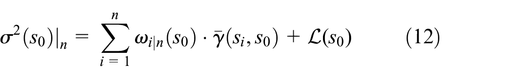
The minimized estimation variance for n sensors, referred to as the OK variance, can be calculated as

$${\sigma }^2\left(s_0\right){|}_n=\sum _{i=1}^n{\omega }_{i|n}\left(s_0\right)·\overline{\gamma }(s_i,s_0)+\mathcal{L}(s_0)$$

(12)

And the whole process of the APCA-OK is displayed in the Algorithm above.

Algorithm APCA-OK
// $\hat{\gamma }(h)$ : EV value // $m(s_i,s_j)$ : similarity between $s_i$ and $s_j$ // p: median of $m(s_i,s_j)$ // $\mathit{R}$ : responsibility matrix // $\mathit{A}$ : availability matrix //t: the times of iteration // $N_{\mathrm{con}}$ : the limitation of the maximum iterative times // $i_{\mathrm{re}}$ : the times of repetitive exemplar // $n_{\mathrm{con}}$ : the limitation of unchanged update times // $\lambda$ : damping coefficient // $N_c$ : number of clusters in the estimation group // $N_n$ : number of sensors in the estimation group // $\hat{z}(s_0){|}_n$ : estimation of field value at $s_0$ based on n sensors // ${\sigma }^2(s_0){|}_n:$ Kriging variance at $s_0$
I:	Calculation of the semivariogram (SV)
1:	Compute the $\hat{\gamma }(h)$ by equation (2).
2:	Obtain the SV by fitting the EV with the spherical model (equation (3)).
II:	Clustering of sensors and formulation of the estimation groups
1:	Compute the similarity $m(s_i,s_j),i\ne j.$
2:	Each diagonal element of similarity matrix is updated by the preference $m(s_i,s_i)$ $\leftarrow p$
3:	Initialization of $\mathit{R}$ and $\mathit{A}$ with zeros.
4:	while $t\le$ $N_{\mathrm{con}}$ or $i_{\mathrm{re}}\le n_{\mathrm{con}}$ do
5:	Compute the $\mathit{R}$ by equation (5).
6:	Compute the $\mathit{A}$ by equations (6) and (7).
7:	Adjust the stability of the iteration by update $\mathit{R}$ and $\mathit{A}$ by   $r_{t+1}(i,j)=\lambda ·r_t(i,j)+(1-\lambda )·r_{t+1}(i,j)$   $a_{t+1}(i,j)=\lambda ·a_t(i,j)+(1-\lambda )·a_{t+1}(i,j).$
8:	Update the $i_{\mathrm{re}}$
9:	t = t + 1
10:	end while
11:	Find the exemplars on the following condition $\mathrm{diag}(\mathit{A}+\mathit{R})>0$ .
12:	Create the index of exemplar of each cluster.
III:	Procession of the OK prediction
1:	for all $s_0$ do
2:	Compute the distances between $s_0$ and each exemplar.
3:	Update the exemplar index in ascending sort of distance.
4:	Select $N_c$ clusters to form the estimation group of $s_0$ based on the distance from each exemplar.
5:	Compute and store the distance between each sensor node in the group by   $d(s_i,s_j)=\Vert s_i-s_j\Vert$ .
6:	Each sensor i computes $\overline{\mathrm{\Gamma }}(s_i,s_j)$ , $\forall j\in N_n$ using stored distanced and SV.
7:	Each sensor i computes $\overline{\gamma }(s_i,s_0).$
8:	Obtain the ${\omega }_{\mathrm{i}|n}(s_0)$ and $\mathcal{L}(s_0)$ by Kriging system (equation (11)).
9:	Compute and store $\hat{z}(s_0){|}_n$ by equation (8) and ${\sigma }^2(s_0){|}_n$ by equation (12).
10:	end for

Simulation and analysis

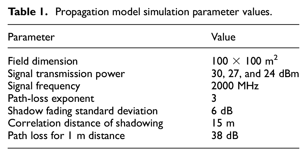
To assess the performance of the proposed APCA-OK algorithm, simulations using MATLAB have been performed on the PC with a processor of AMD Ryzen 7 2700X, 16 GB of memory, and Windows 7 Ultimate operating system, considering the scenario introduced in section “Model and problem statement.” The parameter settings of equation (1) are displayed in Table 1, which is based on the empirical values in the literature.^19,22,23

Table 1.

Propagation model simulation parameter values.

Parameter	Value
Field dimension	100 × 100 m2
Signal transmission power	30, 27, and 24 dBm
Signal frequency	2000 MHz
Path-loss exponent	3
Shadow fading standard deviation	6 dB
Correlation distance of shadowing	15 m
Path loss for 1 m distance	38 dB

After the construction of the scenario, all sensors are placed in the field randomly and clustered by the APCA. Figure 2(a) illustrates random placement when the number of all sensors, N, is 100 while Figure 2(b) illustrates clusters and exemplars of the placement. Since accuracy is a significant criterion to algorithm performance, the mean squared error (MSE) is utilized to analyze the accuracy of REM construction, which can be expressed as follows

$$e_{\mathrm{MSE}}=\frac{1}{l\times w}\sum _{i=1}^l\sum _{j=1}^w{[\hat{z}\left(s_{\mathrm{ij}}\right)-z\left(s_{\mathrm{ij}}\right)]}^2$$

(13)

where l and w are the length and width of the field, respectively, $\hat{z}(s_{\mathrm{ij}})$ is the estimation of interpolation, and $z(s_{\mathrm{ij}})$ is the original value of the simulation. In addition, TC per construction is defined as the time from the beginning of process of measurements to the end of complete REM construction, which is computed by MATLAB functions tic and toc. And it is suitable for describing the relative efficiency of algorithms in simulation. Figure 3 are comparisons of original map between different REM construction results. All of the following data are oriented from multiple simulation results.

Figure 2.

(a) Random placement and (b) AP clustering of sensors N = 100.

Figure 3.

(a) Original map of simulation, (b) IDW, (c) NN, (d) OK, and (e) APCA-OK REM at N = 100 and $N_c=3$ .

Optimal size of estimation group in APCA-OK

The size of estimation group, that is, $N_c$ , number of sensor clusters in each estimation group, is a parameter of importance, which needs to be confirmed before the process of construction. In order to analyze the optimal size, different sizes are compared in the scenario of Table 1 assuming that the number of sensors is 100, which is shown in Figure 4.

Figure 4.

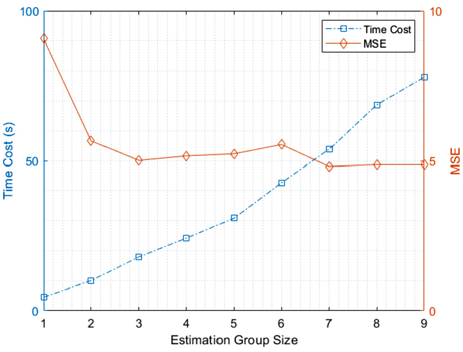
TC and MSE versus estimation group size, N = 100.

As shown in Figure 4, the increase in $N_c$ could reduce the MSE to some extent, but the TC also rises sharply. In this case, when $N_c$ is less than 3, accuracy can be improved significantly, while the TC grows smoothly and MSE reaches its minimum when $N_c$ is 7. A comparison with the situation where $N_c$ is 7 and 3 can illustrate how to confirm the optimal size. Although the former is the most precise, its MSE is just a little smaller than the latter. When it comes to the TC, the former is about 1.5 times more than the latter. Therefore, in this scenario, the optimal size of the estimation group should be 3.

Comparison of TC between OK and APCA-OK

After discussing the optimal size of the estimation group, the computational efficiency of OK and APCA-OK is also crucial, because APCA-OK is provided in order to solve the fast construction problem in dynamic REMs.

As shown in Figure 5, the TCs of OK and APCA-OK are compared in situations with different numbers of sensors. We are informed that APCA-OK always spends less time than OK on REM construction. What’s more, the TC of both methods increases with the increase in the number of sensors, but the gap between the two methods also increases. It is demonstrated clearly that APCA-OK is superior to OK with regard to computational efficiency, and the superiority is more obvious with the increase in the sample ratio of sensors.

Figure 5.

Time cost versus number of sensors.

Comparison of MSEs between different algorithms

According to the analysis above, the superior efficiency of APCA-OK has been proven. But precision is still the most consequential factor in REM application. Therefore, the MSEs are obtained to compare the performance on accuracy of different algorithms, including OK and APCA-OK, and also in addition IDW and NN.

Overall, from Figure 6, the MSE of each algorithm reduces with the increase in number of sensors, which demonstrates that an increase in the sample ratio has a positive effect on construction accuracy. Among these four algorithms, OK and APCA-OK always have less MSE than IDW and NN. OK is slightly more precise than APCA-OK when the number of sensors is less than 100, but this phenomenon reverses when the number of sensors is more than 120, which illustrates that (1) APCA-OK has a similar level of accuracy with OK and is even better with the increase in sample ratio, (2) the estimation accuracy of OK and APCA-OK requires enough measurements for each single unknown point, and (3) the neighbor measurements have much greater influence on both estimation results than the far-away counterpart of unknown points.

Figure 6.

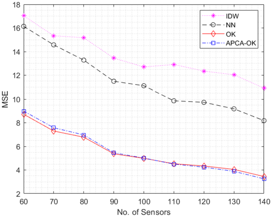
MSE versus number of sensors, $N_c=3$ .

Conclusion

In this article, an adaptive clustering Kriging algorithm in smart sensor networks has been proposed so as to solve the problem of accurate and efficient REM construction for 5G autonomous application. Centralized sensor network is established based on the infrastructure facilities of smart city, and global SV is chosen to represent the spatial correlation of measurements. APCA is utilized to create sensor clusters. The estimation group is formed by comparisons of Kriging variances to add sensors clusters so as to offer a good trade-off between accuracy and computational complexity. Simulation results illustrate the most suitable size of estimation group. APCA-OK outperforms standard OK in terms of efficiency, and it retain the accuracy as the latter. In future work, we will research more on revised REM construction methods for different applications, especially those based on distributed SVs, instead of global ones, for communication terminals scattered in smart city to overcome the constraints resulting from latency in communication channel.