Sage Journals: Discover world-class research

Abstract

Geostatistics has been successfully used to analyse and characterize the spatial variability of environmental properties. Besides providing estimated values at unsampled locations, geostatistics measures the accuracy of the estimate, which is a significant advantage over traditional methods used to assess pollution. This work uses universal block kriging to model and map the spatial distribution of salinity measurements gathered by an Autonomous Underwater Vehicle in a sea outfall monitoring campaign. The aim is to distinguish the effluent plume from the receiving waters, characterizing its spatial variability in the vicinity of the discharge and estimating dilution. The results demonstrate that geostatistical methodology can provide good estimates of the dispersion of effluents, which are valuable in assessing the environmental impact and managing sea outfalls. Moreover, since accurate measurements of the plume's dilution are rare, these studies may be very helpful in the future to validate dispersion models.

Keywords

Autonomous Underwater Vehicles Ordinary And Universal Block Kriging Dilution Estimation Environmental Risk Assessment

1. Introduction

The physical and biological coastal processes that determine the values of environmental variables are complex and still poorly understood. Usually the observations are so unpredictable that the spatial distribution of these variables appears to be random. This randomness makes deterministic solutions adequate to describe the simplest components only [1]. The measurements of environmental variables are usually obtained in very restricted areas and constitute a sample from a continuum that cannot be recorded everywhere. However, people aim to predict the spatial distribution of these variables from a more or less sparse data set. The maps made using the classical methods of spatial interpolation usually display the spatial variation poorly [1]. The interpolators of these methods also fail to provide any estimates of the error, which are desirable for prediction. In this line of thought, geostatistical prediction is the logical solution in the sense that it provides a quantitative description of how the environmental variable differs spatially and a prediction for the places that have not been sampled. Additionally, geostatistics also provides estimates of the errors in these predictions and therefore it is possible to judge how confident we can be about them [1, 2].

Typically, the behaviour of a sea outfall discharge is a process that can be described as follows. The wastewater is usually ejected as an array of turbulent buoyant jets from ports spaced along the outfall diffuser. These turbulent buoyant jets mix with the ambient seawater, usually resulting in rapid reductions of contaminant concentrations. The seawater around coastal outfalls is often density-stratified with density increasing with depth. The discharge, whose density is close to fresh water, is lighter than the surrounding ambient seawater and the plumes rise due to buoyant forces until they reach a level of neutral buoyancy where the effluent spreads laterally, creating a horizontal spreading layer. Depending on the strength of seawater stratification, currents and other variables, the horizontal spreading layer may be submerged and will not be visible on the water surface. If the receiving waters are homogeneous or weakly stratified, the plumes will reach the surface and spread horizontally away from the source [3]. Studying the effluent mixing process in coastal waters in situ is still a complex problem. Several monitoring campaigns using natural tracers have been conducted to detect and map sewage plumes under different oceanic conditions [4 -6]. The results show, however, very complex and patchy structures both in vertical and horizontal sections that are difficult to identify with the classic picture of the buoyant plume. As advanced by several investigations, the observed plume patchiness can occur due to one or a combination of factors which include: (1) variations in currents and stratification during time intervals (which can be hours in some cases), separating the beginning and the end of the field tests and resulting in different equilibrium depths or even distinct plume behaviours, (2) internal tides that can result in a given effluent concentration surface undergoing significant vertical excursions as it advects from the outfall and (3) limitations of sampling in terms of time resolution of time and space scales; in reality, field measurements are not truly synoptic - a transverse of several kilometres can last a couple of hours. Because of their extensive preparation and potentially negative impacts on the environment, detection methods using introduced tracer substances, either at the treatment plant or at the level of the diffusers in the waters, are not practical for routine monitoring of sewage effluents. However, this technique is still the most effective because it makes plume detection easier and usually allows for a quantitative estimation of dilution far away from the diffuser [7-8]. Rapid sampling is expected to reduce time and space variability during and between transects. Because of their easier field logistics, reduced cost per study, increased spatial resolution, reduced spatial aliasing effects and adaptive sampling capabilities, Autonomous Underwater Vehicles (AUVs) are especially valuable in detecting and mapping sewage plumes [9 -13].

2. Geostatistical Prediction

If a stochastic approach is used for the spatial prediction problem, then z( x ), which is a regionalized variable, is seen as a realization of a continuous random function (RF) Z( x ) (i.e., an infinite family of continuous random variables, usually dependent, constructed at all points x of a given domain D one, two or three-dimensional). The set of measured values {z( x _i), i = 1, …, n} is viewed as a collection of several values of z( x ). Each one of these values z( x _i), measured at location x _i, is called a regionalized value. To model the spatial variation of domain D, it is necessary to characterize the RF Z( x ) probabilistically. However, there is little data from one or several realizations of Z( x ) and it would be impossible to infer all the uni- and multivariate distribution functions (for any set of points), unless some assumptions are made. These assumptions are given by the idea of stationarity [1, 14 -16].

2.1 Spatial Correlation

The relationship between two variables (characteristics) can be evaluated using their covariance. For n pairs of observations (z_1,i,z_2,i), i = 1, …, n of two variables z₁ and z₂, the covariance is given by [1]:

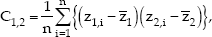
C_{1, 2} = \frac{1}{n} \sum_{i = 1}^{n} {(z_{1, i} - {\bar{z}}_{1}) (z_{2, i} - {\bar{z}}_{2})},

(1)

where ẑ₁ and ẑ₂ are the means of z₁ and z₂, respectively. It is possible to extend this definition to relate any two random variables Z( x _i) and Z( x ) from a RF Z( x ) (where Z( x _i) and Z( x _j) are sets of values of the property Z at the two places x _i and x _j) and their covariance is [1]:

cov (x_{i}, x_{j}) = E [{Z (x_{i}) - μ (x_{i})} {Z (x_{j}) - μ (x_{j})}],

(2)

where μ( x _i) and μ( x _i) are the means of Z at x _i and x _j, respectively. Since it is not possible to know the means μ( x _i) and μ( x _j), the covariance cannot be computed unless some assumptions of stationarity are made. If we assume that: (1) the mean function of the RF is constant for all locations, i.e., [2, 15]:

E [Z (x)] = μ f o r a l l x \in D,

(3)

and that (2) the covariance of Z between any two locations x _i and x _j depends only on their separation h = x _i – x _j, and not on their absolute positions, equation (2) is rewritten as [1]:

cov (x, x + h) = E [Z (x) \cdot Z (x + h)] - μ^{2} = C (h),

(4)

for all x, x + h ∈ D, where the vector h is known as the lag and C( h ) as the covariance function. Equations (3) and (4) are called the hypothesis of second-order stationarity. For a second-order stationary RF, the variance is constant for all x ∈ D and equal to C( o ), the covariance at lag o . In many cases, second-order stationarity is found to be too strong. In some cases, the variance (or dispersion) may be unlimited [16]. For this reason, in [17] Matheron proposed a solution where although in general the mean may not be constant, it would be for small | h | so that the expected differences would be zero:

E [Z (x) - Z (x + h)] = 0 .

(5)

Furthermore, the author replaced the covariances with the variances of differences such as spatial characterization measurements, which, like the covariance, depend on the lag and not on the absolute position [17]:

var [Z (x) - Z (x + h)] = E [{Z (x) - Z (x + h)}^{2}] = 2 γ (h),

(6)

for all X, X + h ∈ D. Equations (5) and (6) are known as the Matheron's intrinsic hypothesis. The quantity γ( h ) is called semi-variance (half the variance) at lag h and, as a function of h , it is called a semi-variogram or simply a variogram. For second-order stationary RFs, the variogram can be computed from the covariance function using the formula [2, 14]:

γ (h) = C (o) - C (h) .

(7)

Under the intrinsic hypothesis the reverse is not true because the covariance function does not exist. The validity of the variogram in a wider range of applications (due to the weaker form of stationarity required for its existence) allow it to be more widely used in geostatistics than the covariance function. However, it has been demonstrated that in practice this is often of no relevance [16]. For a data set |z( x _i),i = 1, …, n}, it is possible to estimate the semi-variance γ( h ) by [1]:

\hat{γ} (h) = \frac{1}{2 N (h)} \sum_{i = 1}^{N (h)} {[z (x_{i}) - z (x_{i} + h)]}^{2},

(8)

where N( h ) is the number of pairs of data points separated by the particular lag vector h . The set of semi-variances obtained by increasing h sequentially constitute the experimental (or sample) variogram. The experimental variogram can be estimated for different directions to enable the identification of directional variation (anisotropy). As well as being a mean to characterize spatial structure, the variogram is also used in the kriging prediction process to obtain semi-variances at particular lags. Therefore, a continuous function must be fitted to the experimental variogram. That function must be such that it will not originate negative variances of random variable combinations. This is guaranteed by ensuring that the covariance function is positive semi-definite and/or the variogram is conditional negative semi-definite (CNSD) [1]. There are two main classes of CNSD functions: bounded models and unbounded models. In bounded models the variance has a maximum, known as a sill. The variogram may reach its sill at a finite lag distance called the range. Alternatively, the variogram may approach its sill asymptotically (in this cases the range is usually taken as the lag at which semi-variance is 0.95 of the sill) or reach a maximum, decrease and perhaps fluctuate about the sill [1]. These variograms are indicative of second-order stationarity and therefore they have equivalent covariance functions. Only pairs of values closer than the range are spatially dependent [16]. In practice, the value at which the model fitted to the variogram crosses the intercept is usually a positive value known as the nugget variance. In most contexts, the nugget effect arises from a spatial variation that has not been resolved due to measurement errors or random variation at lags shorter than the smallest sampling interval [16]. The most common bounded models are spherical, exponential, Gaussian and the Matérn family [1]. Unbounded models do not reach a sill and meet the requirements of intrinsic stationarity only [16]. The simplest and most common models for unbounded variation are the power functions (where the power varies between zero and two) [1]. There are several approaches to fit the models to experimental variograms, but the weighted least squares is the most common method [1]. Kriging is known by the acronym BLUP, which stands for best linear unbiased predictor. The method is best in that it aims to minimize the error variance. It is linear because predictions made using kriging are weighted linear combinations of the sample data available. It is unbiased as it attempts to have a mean residual error equal to zero [16]. All approaches to kriging aim to find the optimal weights λ to assign to n available data z( x _j) to predict the unknown value at the location x ₀. The kriging prediction ẑ( x ₀) is expressed as [15, 16]:

\hat{z} (x_{0}) = \sum_{i = 1}^{n} λ_{i} z (x_{i}) .

(9)

Usually, the n observations used in prediction are at a distance from x ₀ that is smaller than the range. Point (or punctual) kriging makes predictions on the same support as the sample observations. Block kriging is used when the intention is to obtain predictions (averages) over a larger support. Block kriging produces smoother maps than point kriging, as variability is averaged across the larger support [16].

2.2 Ordinary Kriging

Ordinary kriging (OK) is by far the most common type of kriging used in practice. It is based on the assumption that the unknown mean μ is constant across the region of interest, or within the local neighbourhood of the prediction location (which is usually the case) [1, 16].

The predictor must be unbiased and thus the prediction error must have an expected value of zero [15]:

E [\hat{Z} (x_{0}) - Z (x_{0})] = 0 \Rightarrow \sum_{i = 1}^{n} λ_{i} = 1 .

(10)

The kriging (or prediction) variance can be computed in terms of the variogram if condition (10) is used. After some algebra, it is possible to obtain [15]

E [{(\hat{Z} (x_{0}) - Z (x_{0}))}^{2}] = 2 \sum_{i = 1}^{n} λ_{i} γ (x_{i} - x_{0}) - \sum_{i = 1}^{n} \sum_{j = 1}^{n} λ_{i} λ_{j} γ (x_{i} - x_{j}) .

(11)

The values of λ₁, …, λ_n that minimize expression (11) while satisfying constraint (10) are obtained using the Lagrange multipliers method. The conditions for the minimization are given by the OK system of n + 1 equations with n + 1 unknowns [1, 15, 16]:

{\begin{matrix} \sum_{j = 1}^{n} λ_{j} γ (x_{i} - x_{j}) + ψ = γ (x_{i} - x_{0}), i = 1, \dots, n \\ \sum_{j = 1}^{n} λ_{j} = 1 \end{matrix}

(12)

where ψ is the Lagrange multiplier. Its solution provides the weights λ₁, …, λ_n and ψ is the kriging variance given by [1, 15, 16]:

σ_{x_{0}}^{2} = \sum_{i = 1}^{n} λ_{i} γ (x_{i} - x_{0}) + ψ .

(13)

In matrix notation the OK system is written as Ax = b, where A is the n + 1 by n + 1 matrix of semi-variances [1, 15, 16]:

A = [\begin{matrix} γ (x_{1} - x_{1}) & \dots & γ (x_{1} - x_{n}) & 1 \\ ⋮ & ⋮ & ⋮ & ⋮ \\ γ (x_{n} - x_{1}) & \dots & γ (x_{n} - x_{n}) & 1 \\ 1 & \dots & 1 & 0 \end{matrix}],

x are the OK weights and b are semi-variances for the observations for the prediction location:

x = [\begin{matrix} λ_{1} \\ ⋮ \\ λ_{n} \\ ψ \end{matrix}] b = [\begin{matrix} γ (x_{1} - x_{0}) \\ ⋮ \\ γ (x_{n} - x_{0}) \\ 1 \end{matrix}] .

The OK weights are obtained by x = A^–1 b and the kriging variance is given by $σ_{x_{0}}^{2} = b^{T} x .$ . It is easy to see that point kriging is an exact interpolator [1]. A consideration in many environmental applications has been that ordinary kriging usually exhibits large prediction errors [18]. This is due to a larger variability in the observations. When predicting averages over larger areas, that is within blocks, much of the variability averages out and consequently block mean values present lower prediction errors. If the blocks are not too large the spatial patterns do not disappear. The block kriging system is similar to the point kriging system given by (12). The matrix A is the same since it is independent of the location at which the block estimate is required. The semi-variances for vector b are point-to-block semi-variances. Supposing that the mean value over block B is approximated by the arithmetic average of the N point variables contained within that block ([1, 14]), i.e.,

\hat{Z} (B) \approx \frac{1}{N} \sum_{j = 1}^{N} Z (x_{j}),

(14)

then vector b is

b = [\begin{matrix} \bar{γ} (x_{1}, B) \\ ⋮ \\ \bar{γ} (x_{n}, B) \\ 1 \end{matrix}]

where $\bar{γ} (x_{i}, B), i = 1, \dots, n$ is the average semi-variance between the ith sampling point and block B, which can be estimated by:

\bar{γ} (x_{i}, B) = \frac{1}{N} \sum_{j = 1}^{N} γ (x_{i} - x_{j}) .

(15)

The block kriging variance is given by:

σ_{B}^{2} = b^{T} x - \bar{γ} (B, B),

(16)

where $\bar{γ} (B, B)$ is the average semi-variance between pairs of points within B estimated by [1, 14]:

\bar{γ} (B, B) = \frac{1}{N^{2}} \sum_{i = 1}^{N} \sum_{j = 1}^{N} γ (x_{i} - x_{j}) .

(17)

An equivalent procedure, which can be more computationally expensive than block kriging is obtaining the block estimate by averaging the N kriged point estimates within the block [1, 14].

2.3 Kriging in the Presence of Trend

If the variogram increases faster than | h |² for large lags, then the RF is non-stationary [1, 16]. In such cases, the variation in Z( x ) can be modelled as:

Z (x) = m (x) + R (x)

(18)

where R( x ), which is called the residual, is an RF with zero mean and m( x ) is a deterministic function of the coordinates usually expressed as [15]:

m (x) = \sum_{k = 0}^{K} β_{k} f_{k} (x)

(19)

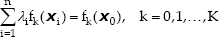
in which β_k are unknown coefficients and f_k( x ) are known functions of the coordinates. Typically the trend m( x ) can be modelled as a low-order polynomial in the spatial coordinates. If K = 0 the model in (18) is stationary with unknown mean β₀, since conventionally f₀( x ) = 1, with the usual variogram and it is therefore possible to use OK. As in OK, the predictor is defined as [1, 15, 16]:

\hat{Z} (x_{0}) = \sum_{i = 1}^{n} λ_{i} Z (x_{i}) .

(20)

The estimator is unbiased if:

\sum_{i = 1}^{n} λ_{i} f_{k} (x_{i}) = f_{k} (x_{0}), k = 0, 1, \dots, K

(21)

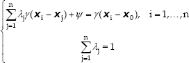
Assuming that R( x ) has a known variogram γ( h ), the kriging variance is given as [1, 15, 16]:

σ_{x_{0}}^{2} = 2 \sum_{i = 1}^{n} λ_{i} γ (x_{i} - x_{0}) - \sum_{i = 1}^{n} \sum_{j = 1}^{n} λ_{i} λ_{j} γ (x_{i} - x_{j}),

(22)

where γ( x _i- x _j) is the semi-variance of the residual between the data points x _i and x _j' and γ( x _i– x ₀) is the semi-variance between the target point x ₀ and the data point x _i. The weights λ₁, …, λ_n are determined using K + 1 Lagrange multipliers (ψ₀,ψ₁, …, ψ_K) and solving the KT (kriging with a trend model or universal kriging) system of n + K +1 equations with n + K + 1 unknowns:

{\begin{matrix} \sum_{j = 1}^{n} λ_{j} γ (x_{i} - x_{j}) + \sum_{k = 0}^{K} ψ_{k} f_{k} (x_{i}) = γ (x_{i} - x_{0}), i = 1, \dots, n \\ \sum_{j = 1}^{n} λ_{j} = 1 \\ \sum_{i = 1}^{n} λ_{i} f_{k} (x_{i}) = f_{k} (x_{0}), k = 0, 1, \dots, K \end{matrix}

(23)

Once the weights and the Lagrange multipliers are known, the kriging variance is given by [1, 15, 16]:

σ_{x_{0}}^{2} = \sum_{k = 0}^{K} ψ_{k} f_{k} (x_{0}) + \sum_{i = 1}^{n} λ_{i} γ (x_{i} - x_{0}) .

(24)

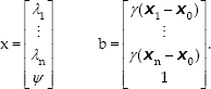
In matrix notation, the KT system is written as Ax = b, where

\begin{array}{l} A = [\begin{matrix} γ (x_{1} - x_{1}) & \dots & γ (x_{1} - x_{n}) & 1 & f_{1} (x_{1}) & \dots & f_{K} (x_{1}) \\ ⋮ & ⋮ & ⋮ & ⋮ & ⋮ & ⋮ & ⋮ \\ γ (x_{n} - x_{1}) & \dots & γ (x_{n} - x_{n}) & 1 & f_{1} (x_{n}) & \dots & f_{K} (x_{n}) \\ 1 & \dots & 1 & 0 & 0 & \dots & 0 \\ f_{1} (x_{1}) & \dots & f_{1} (x_{n}) & 0 & 0 & \dots & 0 \\ ⋮ & \dots & ⋮ & ⋮ & ⋮ & \dots & ⋮ \\ f_{K} (x_{1}) & \dots & f_{K} (x_{n}) & 0 & 0 & \dots & 0 \end{matrix}], \\ x = [\begin{matrix} λ_{1} \\ ⋮ \\ λ_{n} \\ ψ_{0} \\ ψ_{1} \\ ⋮ \\ ψ_{K} \end{matrix}] a n d b = [\begin{matrix} γ (x_{1} - x_{0}) \\ ⋮ \\ γ (x_{n} - x_{0}) \\ 1 \\ f_{1} (x_{0}) \\ ⋮ \\ f_{K} (x_{0}) \end{matrix}] . \end{array}

The KT weights are obtained by x = A^–1 b and the kriging variance is given by $σ_{x_{0}}^{2} = b^{T} x .$ . The equations of block kriging with a trend model (BKT) can be obtained similarly to the ones in block ordinary kriging (BOK). The deterministic component m( x ) may also be a linear expression of one or several variables related to Z. By knowing the values of this (these) variable(s) at data locations, as well as at all locations for which predictions are desired, the form of the equations is the same as for universal kriging. This type of kriging is usually called kriging with external drift (KED).

2.4 Cross Validation

Cross-validation is a procedure used to compare the performance of several competing models. It starts by splitting the data set into two sets: a modelling set and a validation set. Then, the modelling set is used for variogram modelling and kriging in the locations of the validation set. Finally, the measurements of the validation set are compared with their predictions [18]. If the average of the cross-validation errors (or Mean Error, ME) is close to 0

ME = \frac{1}{m} \sum_{i = 1}^{m} [\hat{z} (x_{i}) - z (x_{i})] .

(25)

one may say that apparently the estimates are unbiased (z( x _j) and ẑ( x _j) are, respectively, the measurement and estimate at point x _i and m is the number of measurements in the validation set). A significant negative (positive) mean error represents systematic underestimations (overestimations). The magnitude of the Root Mean Squared Error (RMSE) is particularly interesting for comparing different models [1]:

RMSE = \sqrt{\frac{1}{m} \sum_{i = 1}^{m} {[\hat{z} (x_{i}) - z (x_{i})]}^{2}} .

(26)

The RMSE value should be as small as possible, indicating that estimates are close to measurements. The kriging standard deviation represents the error predicted by the estimation method. Dividing the cross-validation error by the corresponding kriging standard deviation makes it possible to compare the magnitudes of both the actual and predicted error [1]. Therefore, the average of the standardized squared cross-validation errors (or Mean Standardized Squared Error, MSSE)

MSSE = \frac{1}{m} \sum_{i = 1}^{m} \frac{{[\hat{z} (x_{i}) - z (x_{i})]}^{2}}{{\hat{σ}}_{x_{i}}^{2}} .

(27)

should be approximately one, indicating that the model is accurate. A scatterplot of true versus predicted values provides additional evidence on how well an estimation method has performed. Typically the intention is for the set of points to come as close as possible to the line y = x, a 45-degree line passing through the origin of the scatterplot. The coefficient of determination R2 is a good index for summarizing how close the points on the scatterplot come to falling on the 45-degree line passing through the origin [2]. R² should be close to one.

3. MARES AUV

MARES (Modular Autonomous Robot for Environment Sampling) AUV has been successfully used to monitor sea outfall discharges (see Figure 1).

Figure 1.

AUV MARES.

MARES is 1.5m long, it has an 8-inch diameter and weighs about 40kg in air [12, 13]. It features a plastic hull with a dry mid body (for electronics and batteries) and additional rings to accommodate sensors and actuators. Its modular structure simplifies the system's development (the case of adding sensors, for example). It is propelled by two horizontal thrusters located at the rear and two vertical thrusters, one in the front and the other in the rear. This configuration allows for small operational speeds and high manoeuvrability, including pure vertical motions. It is equipped with an omnidirectional acoustic transducer and an electronic system that allows for long baseline navigation. The vehicle can be programmed to follow predefined trajectories while collecting relevant data using the on-board sensors. A Sea-Bird Electronics 49 FastCAT CTD had already been installed on-board the MARES AUV to measure conductivity, temperature and depth. MARES's missions for environmental monitoring of wastewater discharges are conducted using GUI software that fully automates the operational procedures of the campaign. By providing visual and audio information, this software guides the user through a series of steps which include: (1) real time data acquisition from CTD and ADCP sensors, (2) effluent plume parameter modelling using the CTD and ADCP data collected, (3) automatic path creation using the plume model parameters, (4) acoustic buoys and vehicle deployment, (5) automatic acoustic network setup and (6) real time tracking of the AUV mission [13].

4. Results

4.1 Study Site

The study site is shown in Figure 2. The S. Jacinto outfall is located off the Portuguese west coast near the Aveiro estuary [9, 10]. The total length of the outfall, including the diffuser, is 3378m (the first 3135m section has a diameter of 1600mm and the last 243m section has a diameter of 1200mm). The diffuser, which consists of 72 ports alternating on each side, nominally 0.175m in diameter, is 332.5m long. Currently, only the last 20 of the 72 ports are working on a length of 98.2m. The ports are discharging upwards at an angle of 30° to the horizontal axis; the port height is about 1.3m. The outfall has a true bearing direction of 290° and is discharging at a depth varying between approximately 14 and 17m. The sea floor near the diffuser is moderately sloped, with a sandy bottom and isobaths that are parallel to the coastline. In that area the coastline itself runs at about a 200° angle with regard to true north. Flow variation through the outfall in question is not typical of WWTPs since the effluent is mainly of industrial origin. Effluent flow rate ranges most frequently between 0.6 and 0.8m³/s. During the campaign, the discharge remained fairly constant with an average flow rate of ˜0.61 m³/s. Figures 2 and 3 show a plan view of the AUV's position estimate during the plume tracking survey. A rectangular area of approximately 200 × 100m² was covered starting 20m downstream from the middle point of the outfall diffuser. Salinity measurements were obtained at 2 and 4m depths where the effluent plume was predicted to be horizontally dispersing. In each horizontal trajectory, the vehicle described six parallel transects that were perpendicular to the direction of the current, 200m in length and at 20m intervals. When performing horizontal trajectories, vertical oscillations of the AUV were less than 1m (up and down) in the 2m survey and less than 1m down and less than 1.5m up in the 4m survey. In the 2m trajectory, the average depth of the AUV was 2.0m with a standard deviation of 0.20m. In the 4m trajectory, the average depth was 4.0m with a standard deviation of 0.33m. During the mission the vehicle moved at a fairly constant velocity of 1m/s (2 knots). Salinity data were recorded at a rate of 2.4Hz. The geostatistical analysis was conducted using R statistical software and the Gstat package of R [19, 20].

Figure 2.

Plan view of the AUV's position estimate during the plume tracking survey (left). Map of the study site (right).

Figure 3.

Plan view of the AUV's position estimate together with the salinity measurements at 2m (left) and 4m (right) depths.

4.2 Exploratory Analysis

A statistical analysis was conducted in order to obtain elementary knowledge on the conventional salinity data sets (see Table 1 and Figure 4). At a 2m depth the salinity ranged only from 35.152psu to 35.607psu. The mean value of the data set was 35.453psu, which was very close to the median value, which was 35.464psu. The skewness coefficient is relatively low (−0.57), indicating that the distribution is approximately symmetric. The very low value of the variation coefficient (0.0019) reflects the fact that the histogram does not have a tail of high values. At a 4m depth the salinity ranged from 35.097psu to 35.712psu. The mean value of the data set was 35.569psu, which was almost equal to the median value, which was 35.571psu. The skewness coefficient is not very high (−1.32), indicating that the histogram is only slightly asymmetric. The variation coefficient is quite low (0.0015).

Figure 4.

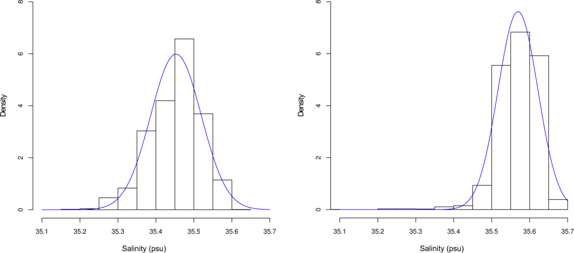
Histograms of salinity measurements at 2m (left) and 4m (right) depths.

Table 1.

Summary statistics of salinity measured at 2 and 4m depths

Summary	Salinity (2m)	Salinity (4m)
Samples	2426	2803
Minimum	35.152 psu	35.097 psu
Lower quartile	35.408 psu	35.538 psu
Mean	35.453 psu	35.569 psu
Upper quartile	35.499 psu	35.609 psu
Median	35.464 psu	35.571 psu
Maximum	35.607 psu	35.712 psu
Skewness coefficient	−0.57	−1.32
Variation coefficient	0.0019	0.0015
Variance	0.00444 psu²	0.00274 psu²
Standard deviation	0.0666 psu	0.0523 psu

The kriging methods work better if the distribution of the data values is close to a normal distribution. Therefore, it is interesting to see how close the distribution of the data values comes to being normal. Figure 4 shows the plots of the normal distribution adjusted to the histograms of the salinity measured at 2 and 4m depths. Apart from some erratic high values, it can be seen that the histograms are reasonably close to the normal distribution. The scatter map at a 2m depth (Figure 3) showed that there might be a trend across the field. That trend is not so evident on the scatter map at a 4m depth. To explore this, the relation between salinity and the Euclidean distance (3D) to the middle point of the diffuser was studied. Figure 5 shows salinity versus the distance at 2 and 4m depths fitted by a linear regression model. It can be seen that salinity increases with the distance and that is more evident at the 2m depth. The Pearson correlation coefficient and the Spearman correlation coefficient between the two variables at the 2m depth are 0.58 and 0.56, respectively. At the 4m depth these coefficients are 0.26 and 0.22, respectively. Therefore, it was decided to assume this trend in subsequent analyses.

Figure 5.

Salinity versus the distance to the middle point of the diffuser at 2m (left) and 4m (right) depths, fitted by a linear model.

4.3 Variogram Modelling

For the purpose of the cross-validation analysis, the salinity measurements were divided into a modelling set (comprising 75% of the samples) and a validation set (comprising 25% of the samples). Modelling and validation sets were then compared in terms of their salinity measurements using the Student's t-test. The aim was to confirm that they provided unbiased sub-sets of the original data. The experimental variograms of both modelling sets (2 and 4m depth) computed using equation (8) are shown as the plotted points in Figure 6 (a) and Figure 7 (a). To explore the trend, experimental variograms of the OLS residuals from the linear model of the Euclidean distance (3D) to the middle point of the diffuser were also computed (see the plotted points in Figure 6 (b) and Figure 7 (b)). The estimation of semi-variance was conducted using a lag distance of 2m and a maximum distance of 120m. Anisotropy was investigated by calculating directional variograms. However, no anisotropy effect could be shown. All experimental variograms were fitted by Matern models (for several shape parameters) using the weighted least squares (WLS) estimation. The parameters of the fitted models are presented in Table 2. At a 2m depth, accounting for the distance to the diffuser has lowered the total variability (as expected from the results of the linear modelling), but it has also reduced the range of spatial dependence. The residual variograms at a 2m depth clearly have a substantially lowered sill and reduced range. At a 4m depth only the range has reduced slightly. All variograms have low nugget values and low nugget/sill ratios. These results indicate that local variations could be captured due to the high sampling rate and the fact that the variable under study has strong spatial dependence.

Figure 6.

Variograms of salinity at 2m depth fitted by Matern models: (a) experimental variogram computed from the raw data using equation (8); (b) experimental variogram of the OLS residuals from a linear trend of the distance to the middle point of the diffuser.

Figure 7.

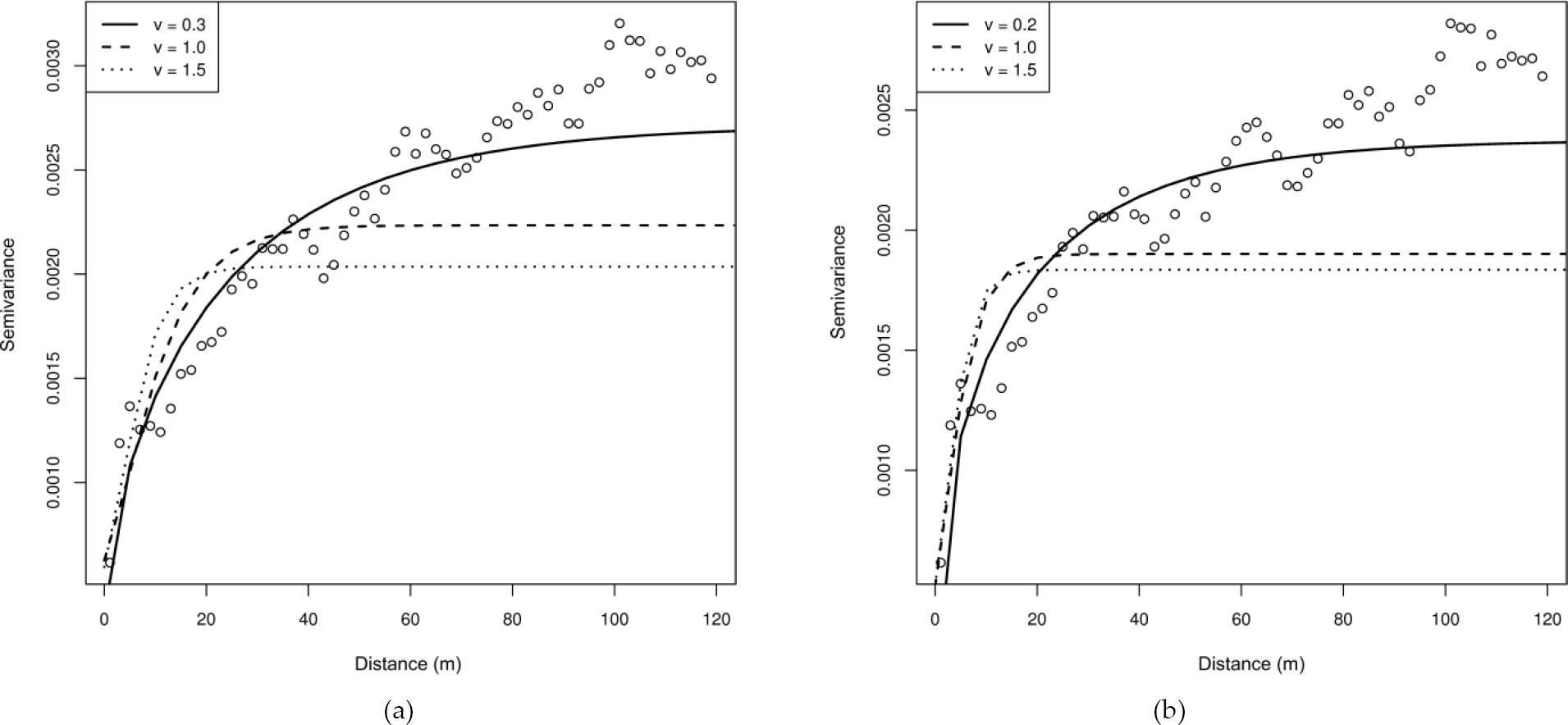
Variograms of salinity at 4m depth fitted by Matern models: (a) experimental variogram computed from the raw data using equation (8); (b) experimental variogram of the OLS residuals from a linear trend of the distance to the middle point of the diffuser.

Table 2.

Parameters of the fitted variogram models for salinity at 2 and 4m depths

Depth	Variogram	Parameter	Nugget	Sill	Range	Nugget/Sill
2m	Raw data	v = 0.6	0.000354	0.017791	204.64	0.019898
		v = 1.0	0.000406	0.008304	55.67	0.048892
		v = 1.5	0.000421	0.007022	34.70	0.059954
	Linear trend	v = 0.3	0.000095	0.002195	37.35	0.043280
		v = 1.0	0.000351	0.001624	10.90	0.216133
		v = 1.5	0.000370	0.001574	8.29	0.235070
4 m	Raw data	v = 0.3	0.000368	0.002346	32.49	0.156863
		v = 1.0	0.000626	0.001608	7.20	0.389303
		v = 1.5	0.000595	0.001441	3.52	0.412908
	Linear trend	v = 0.2	0.000036	0.002339	28.69	0.015391
		v = 1.0	0.000514	0.001387	3.56	0.370584
		v = 1.5	0.000517	0.001318	2.30	0.392261

4.4 Cross-Validation

The block kriging method was preferred since it produced smaller prediction errors and smoother maps in comparison with the point kriging. Using the 75% modelling sets of the two depths and the variograms of the raw data, a two-dimensional Ordinary Block Kriging (BOK), with 10×10 m² blocks, was applied to estimate salinity at the locations of 25% of the validation sets. Using the 75% modelling sets of the two depths and the variograms of the OLS residuals from a linear trend, a two-dimensional Block Kriging with Trend (BKT) with 10×10m² blocks was applied to estimate salinity at the locations of 25% of the validation sets. The measurements of the validation sets were then compared to their predictions. The cross-validation errors computed using Equations 25 -27 are shown in Table 3. For all shape parameters studied, at a 2m depth the salinity was best estimated by the BKT, while at a 4m depth the salinity was best estimated by the OBK. As expected, the BKT performed better than the OBK where the trend was more significant. At a 2m depth, for the best model (v = 0.3), the ME was −0.000997, the RMSE was 0.025023 and the R² value was 0.8621. At a 4m depth, for the best model (v = 1.0), the ME was 0.000004, the RMSE was 0.024242 and the R² value was 0.7706. Both MSSE values are relatively high, probably due to the smoothing effect of the block kriging. Figure 8 shows the scatterplots of true versus estimated values for the most satisfactory models. These plots show once again that observed and predicted values are highly positively correlated. Figure 8 shows the scatterplots of true versus estimated values for the most satisfactory models. These plots show once again that observed and predicted values are highly positively correlated.

Figure 8.

Predicted versus observed salinities at 2m (left) and 4m (right) depths using the preferred models.

Table 3.

Cross-validation results for the salinity measurements at 2 and 4m depths.

Depth	Prediction	Parameter	ME	RMSE	MSSE	R²
2m	BOK	v = 0.6	−0.001091	0.025285	18.23	0.8592
		v = 4	−0.001276	0.025920	30.12	0.8520
		v = 1.5	−0.001468	0.026576	40.71	0.8444
	BKT	v = 0.3^a	−0.000997	0.025023	8.18	0.8621
		v = 1.0	−0.001049	0.025029	17.13	0.8620
		v = 1.5	−0.001111	0.025237	21.52	0.8597
4m	BOK	v = 0.3	0.000069	0.024852	6.51	0.7589
		v = 1.0^a	0.000004	0.024242	9.15	0.7706
		v = 1.5	0.000198	0.024463	7.78	0.7664
	BKT	v = 0.2	0.000102	0.025000	4.88	0.7561
		v = 1.0	0.000180	0.025189	6.73	0.7523
		v = 1.5	0.000294	0.026011	7.03	0.7359

The preferred model.

4.5 Mapping

Figure 9 shows the prediction map of salinity distribution at a 2m depth on a 2×2m² grid, using the BKT with the preferred model. Figure 10 shows the prediction map of salinity distribution at a 4m depth on a 2×2m² grid using the BOK with the preferred model. In the 2m kriged map the average value is 35.447psu and the standard deviation is 0.0610psu, which is in accordance with the salinity measurements (the average value is 35.453psu and the standard deviation is 0.0666psu). In the 4m kriged map the average value is 35.565psu and the standard deviation is 0.0360psu, which is in accordance with the salinity measurements (the average value is 35.569psu and the standard deviation is 0.0523psu). Figure 11 shows the maps of the kriging variance, that is ${\hat{σ}}_{x}^{2},$ , at 2 and 4m depths. In both maps the kriging variance is lower than 0.002 and smaller close to the sampling points, that is, along the trajectory of the vehicle. The kriging variances become large only near the field boundary. In the vicinity of the diffuser, the water column was weakly stratified due to both low temperatures and salinity variations. The total difference in density over the water column was about 0.40σ units. This relatively weak stratification explains the plume spreading near the surface, as predicted by a prediction model used in the field to specify the AUV survey. Both maps show the spatial variation of salinity in the area studied. From these maps it is possible to identify the effluent plume and its dispersion downstream in the direction of the current. It appears as a region of lower salinity when compared to the surrounding ocean waters at the same depth. When considering maximum vertical oscillations of the AUV in performing the horizontal trajectories, the range of background salinity in the 2m map is 35.52 to 35.56psu and the range of background salinity in the 4m map is 35.61 to 35.66psu. When taking the kriging variance into account, in the 2m map the plume may be identified by the regions where salinity is less than 35.48psu and in the 4m map by the regions where salinity is less than 35.57psu. The plume exhibits a considerably more complex structure than the compact shape of the classical picture of the buoyant plume and is as patchy as in previous studies [4 -6]. The small plume-related anomalies in the local salinity of Figures 9 and 10 are evidence of the rapid mixing process. Due to the large differences in density between the rising effluent plume and ambient ocean waters, entrainment and mixing processes are vigorous and the properties within the plume change rapidly [4]. These results therefore confirm that large gradients in background salinity and the small differences in salinity between the effluent plume and the ambient waters can easily obscure the signature of the plume.

Figure 9.

Prediction map of salinity (psu) distribution at 2m depth.

Figure 10.

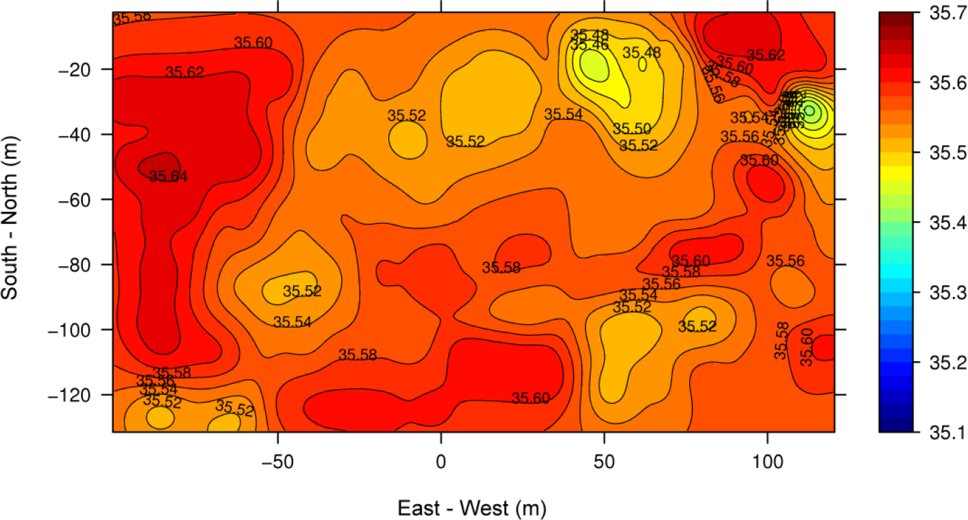
Prediction map of salinity (psu) distribution at 4m depth.

Figure 11.

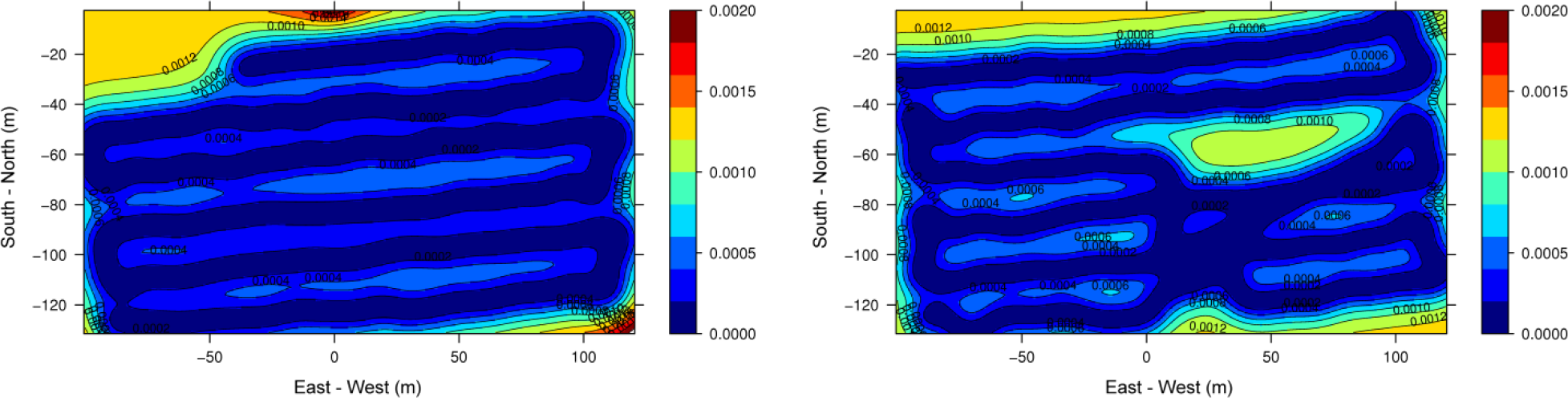
Maps of kriging variance at 2m (left) and 4m (right) depths.

4.6 Dilution Estimation

Environmental effects are all related to concentration C of a particular contaminant X. Defining C_a as the background concentration of substance X in ambient water and C₀ as the concentration of X in the effluent discharge, the local dilution is as follows [21]:

S = \frac{C_{0} - C_{a}}{C - C_{a}} .

(28)

In the case of the variability of the background concentration of substance X in ambient water, the local dilution is given by:

S = \frac{C_{0} - C_{a 0}}{C - C_{a}},

(29)

where C_a0 is the background concentration of substance X in ambient water at the discharge depth. This expression (29) can be arranged to give $C = C_{a} + (\frac{1}{S}) (C_{0} - C_{a 0})$ , which in simple terms means that the increment of the concentration above background is reduced by dilution factor S from the point of discharge to the point of measurement of C. Using salinity distribution at 2 and 4m depths, dilution was estimated using equation (29). The effluent salinity was measured on the day of the campaign at the discharge chamber near the shore using a 24h-composed sample and the average value obtained was 2psu and as a result it was assumed that C₀ = 2.0 psu. A vertical profile of background salinity measured near the discharge indicated 35.54psu at the 2m depth, 35.64psu at the 4m depth and 35.70psu at the discharge depth. As a result, it was assumed that C_a0 = 35.70 psu and C_a = 35.54. At 2 and 4m depths, the result was 35.64psu. The minimum dilution estimated at the 2m depth was about 80:1 and at the 4m depth was about 140:1 (see Figure 12), which is in accordance with the Portuguese legislation that suggests that outfalls should be designed to assure a minimum dilution of 50:1 when the plume reaches surface [22].

Figure 12.

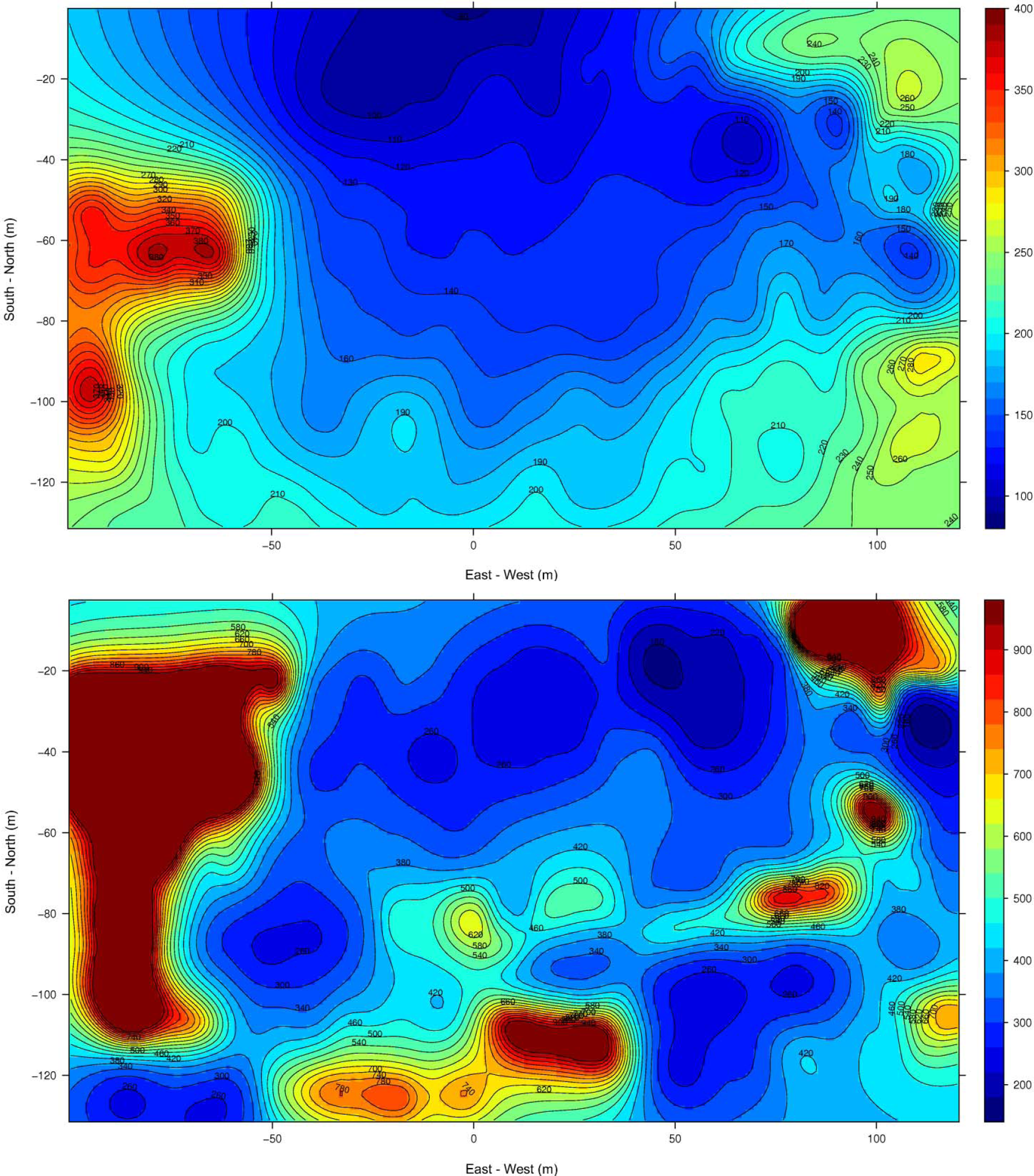
Dilution map at 2m (up) and 4m (down) depths.

4. Conclusions

Through a geostatistical analysis of salinity obtained by an AUV at 2 and 4m depths in an ocean outfall monitoring campaign, it was possible to obtain kriged maps of the sewage dispersion in the field. Experimental variograms of the raw data and of the OLS residuals, from the linear model of the Euclidean distance (3D) to the middle point of diffuser for both depths, were computed and fitted by Matern models for several parameter shapes. The performance of each competing estimator/model was compared using a split-sample approach. The block kriging method was preferred since it produced smaller prediction errors and smoother maps in comparison to point kriging. For all shape parameters studied, at a 2m depth the salinity was best estimated by the BKT, while at a 4m depth the salinity was best estimated by the OBK. As expected, the BKT performed better than the OBK where the trend was more significant. Kriged maps at 2 and 4m depths show the spatial variation of salinity in the area studied and it is possible ability to identify the effluent plume that appears as a region of lower salinity when compared to the surrounding waters. Using the prediction maps of salinity distribution, it was possible to assess the performance of the outfall diffuser by estimating dilution, which in both depths was greater than the minimum admissible value imposed by Portuguese legislation.

Footnotes

5. Acknowledgments

This work was supported by project WWECO-Environmental Assessment and Modelling of Wastewater Discharges using Autonomous Underwater Vehicles Biooptical Observations, funded by the Foundation for Science and Technology (FCT) under the Program for Research Projects in all scientific areas (Programa de Projectos de Investigação em todos os domínos científicos) (ref. PTDC/MAR/74059/2006).

References

Webster

Oliver

M.A

(2007) Geostatistics for environmental scientists, 2nd Edition, John Wiley & Sons, ISBN-13: 978-0-470-02858-2(HB).

Isaaks

E.H

Srivastava

R.M

(1989) Applied geostatistics. Oxford University Press, ISBN 0-19-505012-6-ISBN 0-19-505013-4, 561p.

Tian

Roberts

P.J.W

Daviero

G.J

(2006) Marine Wastewater Discharges from Multiport Diffusers. II: Stratified Flowing Water. Journal of Hydraulic Engineering 132 (4): 411–419. DOI: 10.1061/(ASCE)0733-9429(2006)132:4(411)

Washburn

Jones

B.H

Bratkovich

Dickey

T.D

Chen

M-S

(1992) Mixing, dispersion, and resuspension in vicinity of ocean wastewater plume. Journal of Hydraulic Engineering, ASCE 118 (1): 35–58.

Washburn

Jones

B.H

(1994) Buoyant plume dispersion in a coastal environment: evolving plume structure and dynamics. Continental Shelf Research, 14 (9): 1001–1023.

Petrenko

A.A

Jones

B.H

Dickey

T.D

(1998) Shape and initial dilution of Sand Island, Hawaii sewage plume. Journal of Hydraulic Engineering, ASCE, 124 (6): 565–571.

Carvalho

J.L.B

Roberts

P.J.W

Roldão

(2002) Field Observations of the Ipanema Beach Outfall. Journal of Hydraulic Engineering, ASCE, 128 (2): 151–160.

Hunt

C.D.

Mansfield

A.D.

Mickelson

M.J.

Albro

C.S.

Geyer

W.R.

Roberts

P.J.W

(2010) Plume tracking and dilution of effluent from the Boston sewage outfall. Marine Environmental Research, 70 (2): 150–161.

Ramos

Neves

M.V

Pereira

F.L

(2007) Mapping and Initial Dilution Estimation of a Sewage Outfall Plume using an Autonomous Underwater Vehicle. Continental Shelf Research, 27: 583–593.

10.

Ramos

Neves

M.V

(2009) Environmental Impact Assessment and Management of Sewage Outfall Discharges Using AUV'S. Underwater Vehicles, ISBN: 978-953-7619-49-7, InTech. 417–436.

11.

Rogowski

Terrill

Otero

Hazard

(2011) Mapping Ocean Outfall Plumes and their Mixing using Autonomous Underwater Vehicles. In International Symposium on Outfall Systems, May 15-18, Mar del Plata, Argentina.

12.

Ramos

Abreu

(2011) Using an AUV for assessing wastewater discharges impact: an approach based on geostatistics. Marine Technology Society Journal, 45 (2): 74–87.

13.

Ramos

Abreu

(2011) Mapping and dilution estimation of wastewater discharges based on geostatistics using an Autonomous Underwater Vehicle. Autonomous Underwater Vehicles, ISBN: 978-953-307-432-0, InTech. 239–258.

14.

Goovaerts

(1997) Geostatistics for Natural Resources Evaluation. Oxford University Press, ISBN-10: 0195115384, 496p.

15.

Kitanidis

(1997) Introduction to geostatistics: Applications in hydrogeology. New York (USA), Cambridge University Press, 249p.

16.

Lloyd

(2011) Local Models for Spatial Analysis. CRC Press Taylor & Francis Group, 336p.

17.

Matheron

(1965) Les variables régionalisées et leur estimation: une application de la théorie des fonctions aléatoires aux sciences de la nature. Paris, France: Masson, 305p.

18.

Bivant

R.S

Pebesma

E.J

Gómez-Rubio

(2008) Applied spatial data analysis with R. Springer Series: Use R!, ISBN: 97-0-387-78170-9, 378p.

19.

R Development Core Team, R: a language and environment for statistical computing and graphics . R Foundation for statistical computing. Available: http://www.r-project.org.

20.

Pebesma

E.J

Wesseling

C.G

(1998) Gstat: a program for geostatistical modelling, prediction and simulation. Computers & Geosciences, 24 (1): 17–31.

21.

Fischer

H.B

List

J.E.

Koh

R.C.Y.

Imberger

Brooks

N.H

(1979). Mixing in Inland and Coastal Waters, Academic Press.

22.

INAG (1998). Linhas de Orientação Metodológica para a Elaboração de Estudos Técnicos Necessários para Cumprir o Art^o 7º do D.L. 152/97. Descargas em Zonas Menos Sensíveis, Instituto da Água. Ministério do Ambiente, Lisboa.

Geostatistical Prediction of Ocean Outfall Plume Characteristics Based on an Autonomous Underwater Vehicle

Abstract

Keywords

1. Introduction

2. Geostatistical Prediction

2.1 Spatial Correlation

2.2 Ordinary Kriging

2.3 Kriging in the Presence of Trend

2.4 Cross Validation

3. MARES AUV

4. Results

4.1 Study Site

4.2 Exploratory Analysis

4.3 Variogram Modelling

4.4 Cross-Validation

4.5 Mapping

4.6 Dilution Estimation

4. Conclusions

Footnotes

5. Acknowledgments

References