
Abstract
Histogram shifting is an effective manner to achieve reversible watermarking, which works by shifting pixels between the peak point and its nearest zero point in histogram to make room for watermark embedding. However, once zero point is absent, the algorithm suffers from overflowing problem. Even though some works attempt to deal with this risk by introducing auxiliary information, such as a location map, they occupy a lot of embedding capacity inevitably. In this article, in order to deal with overflowing problem efficiently, we propose a border following–based reversible watermarking algorithm for images. With the help of border following algorithm and pre-processing, available regions with at least one zero point are recognized to embed watermark so that auxiliary information is not needed any more. And the algorithm utilized also ensures the same border can be re-recognized from the watermarked image without error, thus the correctness is also guaranteed. The performance of the proposed algorithm is evaluated using classic image datasets in this area, and the results not only validate the effectiveness of the proposed algorithm but also indicate its advantages compared with the classic histogram shifting–based reversible watermarking algorithm as well as the state of the art.
Introduction
Reversible watermarking1– 6 is an important watermarking technique to achieve information hiding, which enables the cover image to be fully recovered without any distortion once the embedded watermark is extracted. Thus, it has been successfully applied to high-fidelity required environments, such as medical, military, and remote sensing image–based information hiding. For its significant benefit, it is becoming a research hotspot.
Histogram shifting is an effective and important way to achieve reversible watermarking.7–11 It works by shifting pixel values between the peak point and its nearest zero point in histogram of the cover image by “1” to embed watermark. Since watermark is embedded in pixels corresponding to the peak point, great capacity is achieved. However, such a native implementation suffers from the problem of overflowing. Once a histogram does not have a zero point, in order to achieve information hiding, the embedder has to shift pixels between the peak value point and the minimum value point in histogram, thus the pixel values of minimum value point would be permanently corrupted so that the reversibility cannot be ensured any more. As a means to deal with this problem, location information and pixel value of the minimum value point have to be recorded and embedded as auxiliary information, which increases the overhead and occupies the embedding capacity significantly. In addition, some other solutions11–13 have also been proposed to reduce the amount of location information, such as by compression. 13 Although effective, they bring about extra computation cost at the same time. Moreover, auxiliary information is still required in these works, so that the embedding capacity is also affected.
According to a large amount of statistical analysis, even though histogram of the whole cover image does not have a zero point, there is also high probability that at least one zero point exists in a local region of the image. Border following is an effective manner to extract borders of such regions, thus it is a potential way to handle the problem mentioned above effectively. With the help of this technique, borders with at least one zero-value pixel inside can be recognized. By embedding watermark bits inside, auxiliary information such as location map is not needed any more, thus achieving high efficiency and large embedding capacity. In this article, we propose a border following–based reversible watermarking algorithm for images with resistance to histogram overflowing. The proposed algorithm is not only effective, but also lightweight. Our major contributions can be summarized as follows:
We present a novel framework to support border following–based reversible watermarking mechanism, which consists of an image pre-processing module, a histogram shifting–based watermark embedding module, and a watermark extracting module. Furthermore, specific algorithms for all of them are presented respectively.
We propose a border following–based reversible watermarking algorithm based on histogram shifting, which is able to resist against overflowing problem with only a small amount of computational overhead required to extract borders. It filtrates images and selects available regions adaptively to embed watermark. To avoid overflowing, the histogram of selected region is ensured to have at least one zero point. Clearly, watermark can be embedded into multiple regions in a single image simultaneously to achieve large capacity as long as they satisfy the requirement.
We verify effectiveness of the proposed algorithm and compare it with the state of the art by experiments. Experimental results show that our presented algorithm is fully reversible and overflowing problem is avoided with only small amount of overhead required.
Related works
Ni et al. 14 proposed the first histogram shifting–based reversible watermarking algorithm, which embeds watermark by modifying pixel values of the cover image between the peak point and its nearest zero point in the histogram. However, for a histogram without zero point, to handle overflowing problem, the scheme has to record and embed location information as well as pixel value of the minimum value point as auxiliary information, which introduces a great amount of extra overhead inevitably. On the basis of their work, to improve imperceptibility, Wang et al. 15 optimized rate and distortion for histogram shifting–based algorithms. Chen et al. 12 reduced the extra information by only recording pixels that have been moved. However, to resist overflowing, these methods also have to generate and embed a location map as auxiliary information.
On the other hand, Fu et al. 11 presented a novel reversible watermarking algorithm based on prediction-error histogram shifting as well as exploiting modification direction (EMD) mechanism. They exploit the similarity among adjacent pixels and use the side-match predictors to obtain prediction-error histogram, then embed watermark by shifting this histogram. Thanks to the nonary EMD algorithm and the multi-layer embedding mechanism, the capacity of the proposed method is greatly improved. However, to resist overflowing problem, auxiliary information is still necessary. In addition, Xuan et al. 16 proposed a histogram-pair-based image reversible data hiding scheme, which embeds data into the prediction errors generated from a cover image. To avoid overflowing, it shrinks the histogram to generate zero point before data embedding, which requires large amounts of computational overhead.
Furthermore, Kim et al. 17 proposed a gradient-adjusted prediction (GAP) and modulo operation–based solution to provide superior image quality and large capacity. However, the reversibility of the proposed scheme still replies on the existence of zero value points in the histogram. As further development, Caciula et al. 18 investigated a multiple moduli prediction error expansion approach to achieve reversible data hiding. Thanks to the introduced linear programming model, the specific moduli is selected so as to maximize the embedding bit rate. In order to ensure reversibility, a location map with the expansion information is embedded together with the payload. In this case, auxiliary information is still inevitable.
Moreover, Sachnev et al. 19 proposed a new rhombus prediction scheme to improve efficiency, which employs sorted prediction errors to reach balance between capacity and imperceptibility. Based on their work, Kim et al. 13 proposed a skewed histogram shifting–based embedding framework, which utilizes a pair of extreme predictions. Specifically, only pixels from the peak and short tail are used for embedding, which decreases the distortion from the lesser number of pixels being shifted. However, a location map as auxiliary information is still necessary. Moreover, in order to compress the location map, extra computation overhead is also introduced.
In this article, to deal with security and efficiency problems mentioned above, we propose a border following–based reversible watermarking algorithm for images, which is able to avoid overflowing without introducing auxiliary information. Specifically, once the zero value point is absent in histogram of the cover image, we utilize image pre-processing to make sure there is at least one zero point inside the recognized border.
Reversible watermarking algorithm based on border following
In this article, we propose a border following–based reversible watermarking algorithm for images. The algorithm employs border following to obtain available regions inside of the border. In order to ensure large capacity, peak point of each region is utilized to embed watermark by histogram shifting. To extract watermark, the receiver performs the same border following algorithm to find out the watermarked region inside of the border, which is ensured to be identical with the one recognized from the un-watermarked image under the algorithm. Thus, reversible extraction of the watermark is guaranteed.
Figure 1 is an illustration of the proposed reversible watermarking algorithm. From the flowchart, it is clear that the algorithm consists of three parts: image pre-processing, histogram shifting–based watermark embedding, and watermark extracting. For cover images, we first employ the Otsu method 20 to get the threshold value, which is utilized to convert cover images into binary ones, ensuring the variance of divided pixels in two categories to be maximized. With the help of this method, pixels inside the recognized border are more similar with each other, thus raising the number of peak points in the corresponding histogram with high probability. After successfully identifying the borders in the image, check the number of zero value pixels inside each border to determine whether the image is available. Two simplified examples of available and unavailable images are shown in image pre-processing module. On finishing pre-processing of available images, histograms of pixels inside each recognized border are generated. Due to the limitation of space, histograms are just schematic diagrams and have no direct correspondence with specific regions in the example shown before. Then, watermark bits are embedded based on histogram shifting. For a watermarked image, execute the same procedure of border following to detect borders and then extract watermark from the inside pixels to obtain the recovered image. During the whole procedure, border following algorithm introduced below is the key to achieve resistance against histogram overflowing.

Framework of our proposed algorithm.
Semantic segmentation model–based border following algorithm
As a preparation for the proposed border following–based reversible watermarking algorithm to deal with histogram overflowing, we need such a semantic segmentation model–based border following algorithm 21 as preliminary. In order to segment an image according to semantics, the algorithm first transforms it into a binary one and temporarily expands the image by 0 to deal with pixels on its four boundaries. Then raster scans the original binary image without the expanded scope in pixel level to achieve border following. Once a pixel with value 1 is encountered, it takes the pixel as the center of a 3 × 3 matrix and checks the 8 pixels around. If all of them are zero point, the central pixel is set to −2 to indicate the recognized single pixel. Otherwise, take the current pixel as the center and the first non-zero pixel encountered as the start point, which is scanned in clockwise order from the left pixel of the center. Check the matrix in anti-clockwise order from the chosen start point and select the first non-zero pixel as the next central pixel. Meanwhile, set the current central pixel as the start point for the next round. Specifically, in the latter case, the central pixel is marked as 2 if the value of its right adjacent pixel is non-zero, or marked as −2 otherwise. Repeat the above procedures until scanning to the start point in the first round. Once finishing a complete border following, the algorithm starts a new raster scanning from the right adjacent pixel of the first start point, thus ensuring that none of the previous border pixels are involved in the next 3 × 3 matrix selected. It is worth noting that, since border following algorithm always begins from the first 1-value pixel in each line scanned, even if pixel values inside the recognized region are changed, the position of the border could also be accurately recognized. In order to demonstrate the effect of the algorithm intuitively, we take a 5 × 5 binary image shown in Figure 2 as an example and implement the border following algorithm on it. We first expand the image with 0 pixels in grids surrounded by dotted lines to a 7 × 7 one, in order to implement border following algorithm on original boundaries of the image. Figure 2 shows the first two rounds of border following and the outermost border of the recognized region is marked in Figure 3. After performing the algorithm on the whole image, the expanded grids with 0 pixels inside are eliminated. In this way, expanded boundaries are just employed to ensure the execution of border following on original boundaries, rather than involving in subsequent data processing which may introduce extra overhead. Due to its robustness and reliability, the algorithm has already been widely used in component counting and topological structural analysis of digital images.

Pixels of a binary image.

Border presentation of the binary image.
Image pre-processing
We first transform cover images into binary ones and mark the outermost border of the recognized region in border presentation. In order to resist histogram overflowing, we first find out images whose recognized regions contain at least one zero point. Then select them and keep their border coordinate points as preparation. Pixels inside each of the border are employed to embed watermark. Below we introduce the image pre-processing procedure in more detail.
Step 1. To convert an M × N cover image I into a binary one, we first employ the Otsu method
20
to get the binary threshold t. Under the value, the pixels of Image I are divided into two categories, between which the variance is ensured to be maximized. Then scan pixels of I in a raster order. Compare pixel value
Step 2. In order to cover pixels on the boundary of the original image, expand its four boundaries with zero-value pixels to get the expanded (M + 2) × (N + 2) image
Step 3. Raster scan
As is shown in Figure 4(c), take

Select the first non-zero pixel as the next central pixel, and the current central pixel as the start point. Scan pixels in anti-clockwise order again and update the value of central pixel. The scanning process is shown in Figure 4(d). Repeat the above process until scanning to the start point
Step 4. Start a new raster scanning from the right adjacent pixel
Step 5. On finishing border following of the cover image, update the marked border with its absolute value to make sure the marked value is constant even though watermark bits are embedded inside. Show the updated border in Figures 4(l) and 5(d).
Step 6. In order to ensure the feasibility of border following after watermark embedding and the reversible extraction in corresponding regions, sort each border according to the size of region it enclosed. If at least one zero-value pixel exists inside of the largest k borders, denote them as
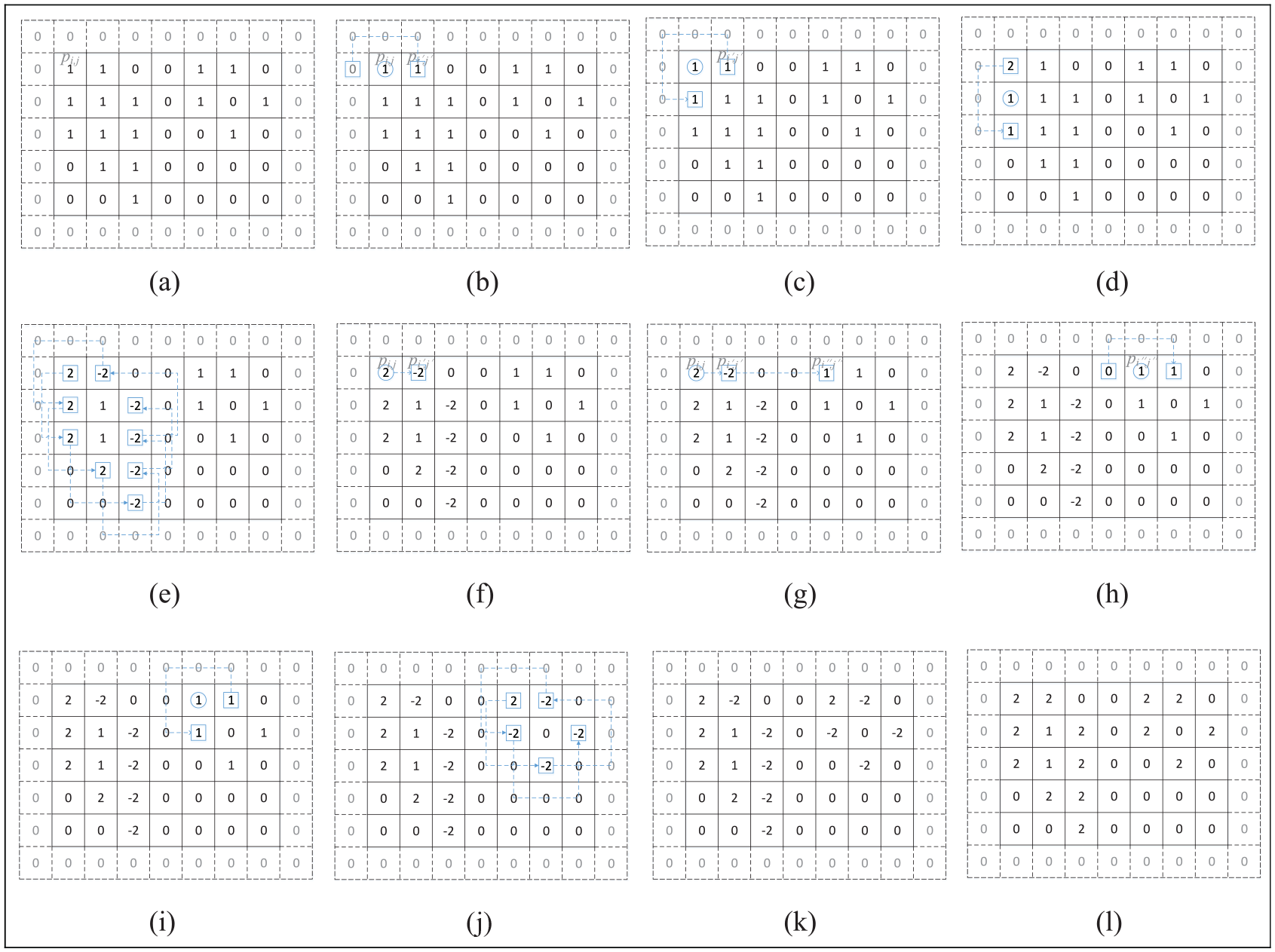
Border following of regions: (a) pixels of a binary image, (b) clockwise scanning, (c) first anti-clockwise scanning, (d) second anti-clockwise scanning, (e) first-border presentation, (f) end of first round scanning, (g) find a new border, (h) clockwise scanning of the new border, (i) first anti-clockwise scanning of the new border, (j) second-border presentation, (k) end of second round scanning, and (l) marked border with its absolute value.

Border following of a single pixel: (a) pixels of a binary image, (b) clockwise scanning, (c) border presentation, and (d) marked border with its absolute value.
Watermark embedding based on histogram shifting
According to the procedure of image pre-processing, at least one zero point exists inside of the recognized border. Denote the pixel value of peak-value point as
Notations used in this article.

In order to embed watermark into I, we first scan pixels inside of each border
Histogram shifting.
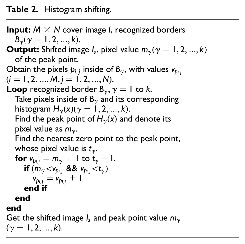
Watermark embedding.

Step 1. Generate histograms of pixels inside of each border

Step 2. Scan pixels inside of
Watermark extraction and recovery of cover image
Once receiving a watermarked image
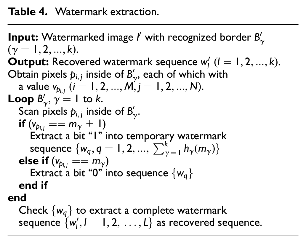
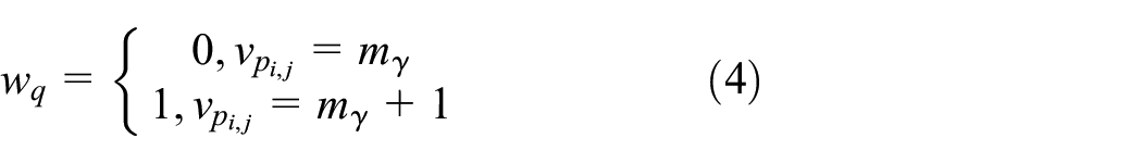
We first scan pixels inside of each
Watermark extraction.
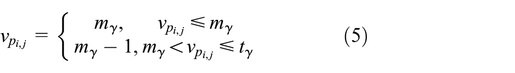
Cover image recovery.
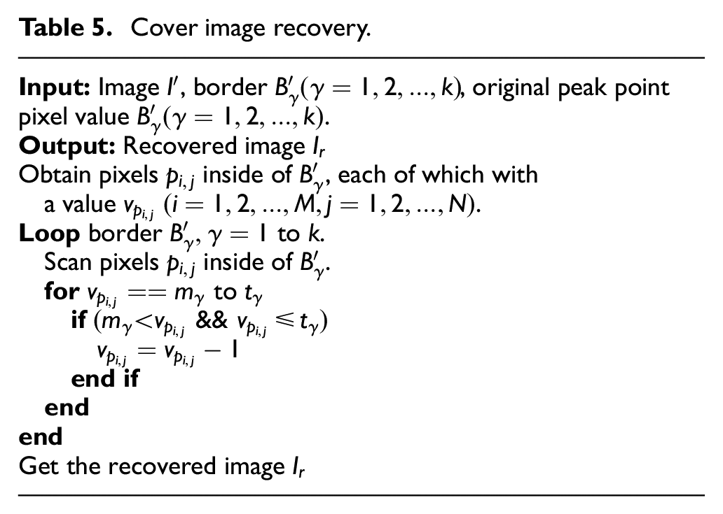
Step 1. Scan pixels inside of
Step 2. Scan the pixels inside of
Step 3. On finishing extracting from
Security analysis
To evaluate the security of the proposed algorithm, we consider three types of attackers. The first type intercepts the watermarked image and wants to steal the content of the watermark. The latter two focus on specific types of watermarks. For the second type, the attackers aim at the watermark used for copyright protection. In order to abuse the content of images, it is devoted to destroy the watermark while keeping the cover image unchanged. While for the third one, they contrapose the watermark used for tampering detection. In this case, the watermark embedded may be the hash value of the content of cover image. On receiving the watermarked image, the attacker extracts the watermark to recover the cover image. Then it tampers the recovered image and re-generates its hash value before embedding. Obviously, the watermarked image would pass the process of tampering detection even though the content of which is tampered.
For the first type of attackers, they are completely able to obtain the threshold value at first by employing the Otsu method 20 and then recognize watermarked regions with the help of border following algorithm. However, the watermark still cannot be successfully extracted on account that the positions of peak value point as well as zero value point before embedding are actually unknown to attackers. In this scenario, the security of the proposed algorithm is equal to histogram shifting–based ones, rather than being affected by the introduced image binarization and border following methods. As for the second type of attackers, once they destroy the watermark embedded, the cover image is actually not able to be recovered without error, which is ensured by the principle of reversible watermark algorithms, thus the security is guaranteed. For the third one, attackers have to extract watermark first. Due to the same reason mentioned above for the first type of attackers, watermark cannot be extracted since the previous positions of both peak and zero points are still unknown. As a result, security of the proposed algorithm is always guaranteed against three types of attackers mentioned above.
Experiments and results
In this section, we take experiments to validate the effectiveness and evaluate the efficiency of the proposed border following–based reversible watermarking algorithm. Our watermark embedding and extracting procedures are considered to be executed by sender and receiver of the watermarked image, respectively. In this section, we employ a workstation with Intel(R) Core (TM) i7-6700 CPU @3.40 GHz, 8GB RAM, and a 7200 RPM 1TB hard drive to implement both of them. All algorithms are implemented using MATLAB 2019a and Python version 3.7. We perform our experiments on three image datasets: Boss dataset, 22 Caltech 101 dataset, 23 and Oxford5k dataset, 24 in which the first one contains 40,000 images, the second one 9144 images, while the third one 5062 images. All results are on the average of 20 tries.
Watermark embedding and extracting
In this part, we first choose an image shown in Figure 6(a) from the Oxford5k dataset. According to its histogram in Figure 7, zero-value pixel is absent, which means the algorithm proposed by Ni et al. 14 is not applicable any more. We execute the pre-processing procedure and transform the image into a binary one shown in Figure 6(b). Specifically, we exhibit three largest available regions recognized under the border following algorithm and mark their respective borders in Figure 6(c). The relationship between the number of available regions and performance of the proposed algorithm is also evaluated in detail in next part of the experiment.

Un-watermarked images: (a) original image, (b) binary image, and (c) recognized borders in the image.

Histogram of original image.
We exhibit the pixels inside of each recognized border in Figure 8(a), (c), and (e), each of which is paired with the corresponding histogram, as is shown in Figure 8(b), (d), and (f). For each histogram, it contains 4, 50, and 121 zero value pixels, and the value of peak point is 3180, 456, and 1151, respectively, which means overflowing problem is avoided and embedding capacity is guaranteed if watermark bits are embedded in these regions. Embed watermark sequence iteratively by histogram shifting–based embedding method introduced above until every one of the embeddable positions are occupied. For the watermarked image shown in Figure 9, we re-recognized the borders by the border following algorithm and showed the watermarked pixels inside in Figure 10(a), (c), and (e) respectively, together with their histograms in Figure 10(b), (d), and (f).

Un-watermarked regions and corresponding histograms: (a) region 1, (b) histogram of region 1, (c) region 2, (d) histogram of region 2, (e) region 3, and (f) histogram of region 3.

Watermarked image.

Watermarked regions and corresponding histograms: (a) region 1, (b) histogram of region 1, (c) region 2, (d) histogram of region 2, (e) region 3, and (f) histogram of region 3.
To validate the effectiveness of our proposed algorithm, we first verify whether the border could still be recognized by executing border following algorithm employed introduced above. According to the image pre-processing, it is clear that even if pixels inside of each region may change after watermark embedding, the largest three borders can still be accurately recognized by the receiver based on the agreement with the sender on the number of borders, for the reason that pixels of the borders are not embedded. The recognized borders in the watermarked image are shown in Figure 11.

Recognized borders in the watermarked image.
For a selected cover image, present its extracted borders and the ones from its watermarked version in Figure 12(a) and (b), respectively. To demonstrate whether the latter one is identical to the former one, perform exclusive OR operation on them and show the result in Figure 12(c), which is a binary image. Since the result image is all black, the re-recognized borders are validated to be the same as previous ones, which means watermark embedding does not affect border following procedure and our proposed algorithm is effective.

Extracted borders and result of exclusive OR: (a) border of un-watermarked image, (b) border of watermarked image, and (c) result of exclusive OR.
Then, Figure 13(a) exhibits extracted borders and regions inside of each one, while Figure 13(b) shows the ones from the watermarked image. To further demonstrate whether the watermark is embedded, perform exclusive OR operation on them and the result is shown in Figure 13(c). Inferring from Figures 12(c) and 13(c), we can eventually draw the conclusion that the borders are identical before and after watermark embedding.

Extracted borders with pixels inside and result of exclusive OR: (a) unwatermarked regions, (b) watermarked regions, and (c) result of exclusive OR.
Finally, the process of image recovery is shown in Figure 14(a)–(d). Figure 14(a) exhibits the un-watermarked regions of the cover image. As the inverse process of embedding, we extract watermark bits from pixels inside of the re-recognized three borders, respectively, to recover the corresponding regions. Then we put the recovered regions back into the original image successively. The process is shown in Figure 14(b)–(d). It is worth noting that Figure 14(d) is the fully recovered image and it is completely consistent with the original image which is guaranteed by the principle of histogram shifting–based reversible watermarking.

Process of image recovery and recovered image: (a) unrecovered image, (b) recover region 1, (c) recover region 2, and (d) recover region 3.
Performance evaluation
In this part, we compare our proposed algorithm with the classic histogram shifting–based reversible watermarking algorithm as well as the state of the art. In order to evaluate performance as objective as possible, we implement our algorithm together with algorithms proposed by Ni et al. 14 and Kim et al. 13 based on the three selected classic image datasets.
Availability of images in datasets
As the first step, we find out available images for our algorithm and Ni’s algorithm 14 from the selected datasets separately and compare availability. To ensure embedding capacity, we set the number of available borders in a single image to be 3, even though a few regions to be embedded means better performance to our algorithm. The result is shown in Figure 15, in the form of histogram pairs.

Percentage of available images.
According to Figure 15, the percentage of available images to our algorithm is 94.75%, 67.81%, and 51.55% for Boss dataset, Caltech 101 dataset, and Oxford5k dataset, respectively. The ratio drops to 82.65%, 58.67%, and 32.71% for Ni’s algorithm. The reason lies in that Ni’s algorithm requires the existence of at least one zero-value point in histogram of the cover image. And for our proposed algorithm, the image is available as long as at least one zero point exists inside of the recognized border. Therefore, even if the whole image does not have a zero point, it is still possible to satisfy the requirements of our algorithm.
Imperceptibility of the proposed algorithm
Next, we compare the imperceptibility of our proposed algorithm and Kim’s algorithm 13 under the same amount of watermark bits embedded. In order to keep the computational overhead comparable for both algorithms, in Kim’s algorithm, we embed location map directly into cover image without compression.
We randomly take out 12 available images from the selected three image datasets, respectively, each of which with 4 pieces. The images selected are shown in Figures 16–18. We restrict the amount of watermark bits embedded of both algorithms to be 1000, 2000, 3000, and 4000 bits, respectively, and compare the corresponding imperceptibility, which is evaluated by peak signal-to-noise ratio (PSNR) (dB). The result is shown in Table 6.

Test images from Boss dataset: (a) building, (b) bell tower, (c) mountain, and (d) canyon.

Test images from Caltech 101 dataset: (a) small-sized passenger aircraft, (b) medium-sized passenger aircraft, (c) fighter, and (d) transport plane.

Test images from Oxford5k dataset: (a) dining room, (b) teaching building, (c) campus, and (d) church.
Comparison of imperceptibility.
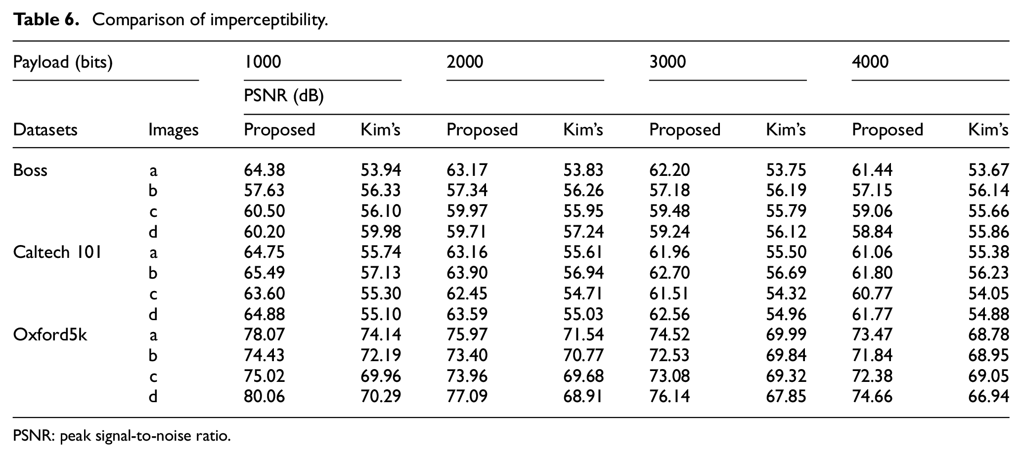
PSNR: peak signal-to-noise ratio.
According to the table, the PSNR of our algorithm is obviously higher than Kim’s work. 13 For example, for the first selected image in Boss dataset, the PSNR of our algorithm is 64.38, 63.17, 62.20, and 61.44 dB for the payload of 1000, 2000, 3000, and 4000 bits, respectively, which is obviously higher than 53.94, 53.83, 53.75, and 53.67 dB for Kim’s algorithm. The reason is that in order to resist overflowing, Kim et al. embed a location map as auxiliary information into the cover image, which occupies large amounts of embedding space. And for our proposed algorithm, auxiliary information is not needed any more so that for the same quantity of watermark bits embedded, fewer pixels are shifted thus a better imperceptibility is guaranteed.
Relationship between binary threshold value and embedding capacity
Finally, we explore the relationship between binary threshold value t and embedding capacity C of the cover image. In order to evaluate correlation of the number of recognized borders and capacity simultaneously, we divide the 12 pieces of images employed above into three categories according to datasets and restrict the number k to be 1, 2, and 3 to calculate the average embedding capacity of three groups under different t, respectively. The result is shown in Figure 19(a)–(c).

The relationship between binary threshold value and embedding capacity: (a) Boss dataset, (b) Caltech 101 dataset, and (c) Oxford5k dataset.
Referring to these figures, we find the general trend is that the average embedding capacity of each group increases with the number k in general. For example, in Figure 19(a), compared with the curve k = 1, when k = 2, the capacity (bits) increases from [7430, 9777] to [7818, 9794]. And once k = 3, the capacity is even greater. This is because in our scheme, larger k means more regions recognized in the cover image could be employed to embed watermark. Moreover, we can also find in the figure, in some selected values of t, various k corresponds to the same capacity, for example, under threshold t = 10, the curve of k = 2 overlaps with the curve of k = 3. This is because in this case, the number of recognized regions is actually 2. According to the result obtained, we can conclude that the embedding capacity of our proposed algorithm is flexible, which means once more regions recognized by border following algorithm are employed, the capacity of our algorithm still has room to improve. Finally, it is clear that the capacity C decreases with the increase of threshold value t. The reason is that, in our algorithm, the capacity is determined by the number of peak-value points, which is largely affected by the size of recognized regions. According to the principle of border following algorithm utilized, a smaller value of t means more pixels in the cover image are marked with 1, thus larger recognized regions could be obtained.
Universality of image binarization
In order to validate the universality of our proposed algorithm, we employ the Otsu method to generate binary threshold values for the selected 12 images, respectively. Then, we calculate the embedding capacity for each of them under the corresponding threshold value, and the average capacity for each group under different k. The result is shown in Table 7.
The relationship between binary threshold value and average embedding capacity.
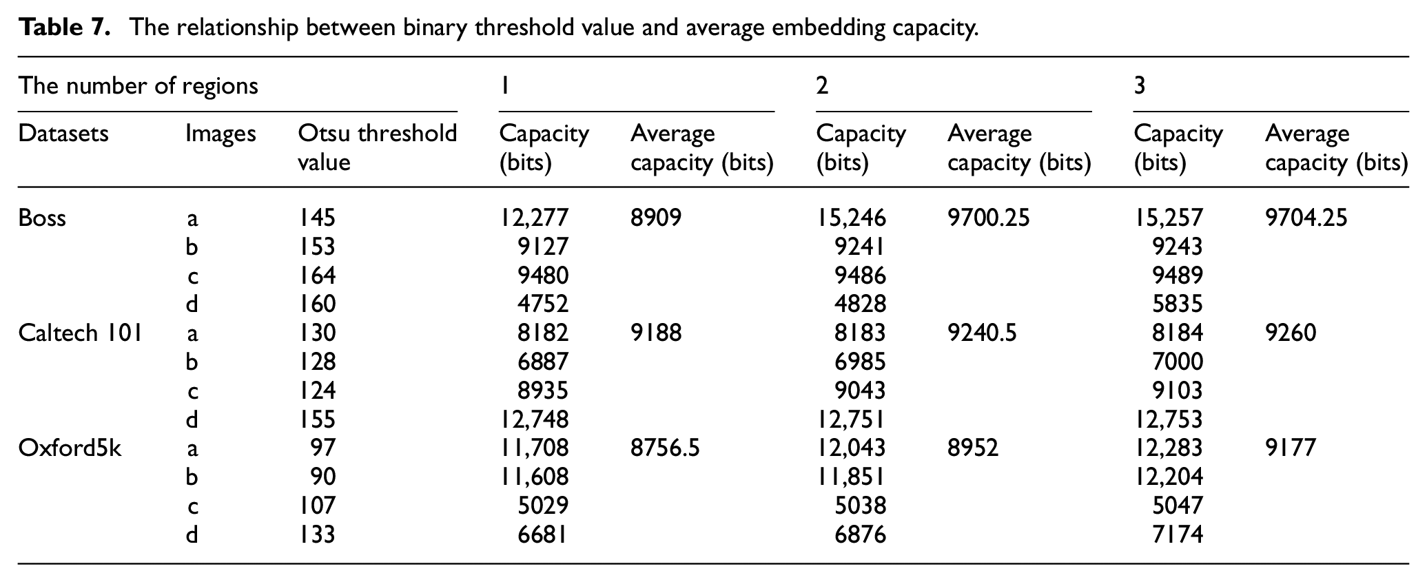
According to the table, for Boss dataset, restrict the number k to be 1, 2, 3, the average embedding capacities are 8909, 9700.25, and 9704.25 bits, which are very close to the maximum values 9777.5, 9794, and 9796 bits in Figure 19(a). As for Caltech 101 dataset, the values change to 9188, 9240.5, and 9260 bits, which are also very close to the corresponding maximum average embedding capacities 9199, 9248.25, and 9301.5 bits in Figure 19(b). However, for Oxford5k dataset, restrict the number k to be 1, 2, 3, the average embedding capacities are 8756.5, 8952, and 9177 bits, which are lower than the maximum values 14,015.25, 14,111.75, and 14,230.75 bits in Figure 19(c).
The reason is that the Otsu method only ensures pixels in each one of the categories are as similar as possible. A natural result is that the number of peak point pixels in each category is maximized with high probability, which is the basic guarantee to achieve large capacity. However, it is not enough since that the capacity is actually determined by the number of peak point pixels inside of the regions recognized by border following algorithm. On calculating the threshold value, for images with good contrast ratio, pixels are ensured to be divided as accurately as possible, thus raising the possibility to achieve high capacity. On the other hand, for those with bad contrast ratio, due to the inherent defects of the Otsu method, image details are easy to be lost, resulting in the poor continuity of the region recognized by the border following algorithm, thus affecting the embedding capacity. However, Otsu method is still the most outstanding representative of binarization algorithm for gray scale images. Therefore, thanks to superior contrast ratio of images in both Boss and Caltech 101 datasets, they are with high capacity under the employed Otsu threshold value. While for Oxford5k dataset, the capacity drops rapidly due to worse contrast ratio. Despite the above problem, we still achieve fairly good performance since the average capacity for images in Oxford5k dataset reaches the average level in Figure 19(c).
Conclusion
In this article, we propose a novel histogram shifting–based reversible watermarking algorithm for images to resist overflowing problem. Specifically, we utilize border following algorithm to find out appropriate regions in the cover image for watermark embedding, thus auxiliary information is not needed any more. Our algorithm is compared with the classic histogram shifting–based reversible watermarking algorithm as well as the state of the art through experiments and the results show that the proposed algorithm has better performance.
Footnotes
Handling Editor: Hongxin Hu
Declaration of conflicting interests
The author(s) declared no potential conflicts of interest with respect to the research, authorship, and/or publication of this article.
Funding
The author(s) disclosed receipt of the following financial support for the research, authorship, and/or publication of this article: This work was supported in part by Construction of advanced disciplines for University of International Relations under Grant No. 2019GA36, the National Natural Science Foundation of China under Grant U1536207, in part by the Fundamental Research Funds for the Central Universities, University of International Relations, under Grant 3262019T68, and in part by the National Key R & D Plan of China under Grants 2016QY04W0803 and 2016YFB0800402.