
Abstract
Partial discharges are the main insulation defects encountered in gas-insulated switchgears. When it occurs inside the gas-insulated switchgear cavity, it degrades insulation, and, sooner or later, causes a breakdown. Therefore, it is important to discover insulation defects as early as possible, locate the discharge, and perform both defect identification and maintenance. Current ultra high frequency-based partial discharge location methods mainly use time delay. To obtain accurate delay times, however, a very high sampling rate is needed, which requires expensive hardware and greatly limits its application. Therefore, in this article, a localization method based on received signal strength indicator ranging is proposed, and location estimation is carried out. An easily implementable particle swarm optimization algorithm with high positioning accuracy is selected to compensate for the low positioning accuracy of current received signal strength indicator ranging methods. To further improve positioning accuracy, the convergence conditions of the particle swarm optimization are investigated, and, considering their constraints, an improved particle swarm optimization algorithm is proposed. By combining the characteristics of ultra high frequency wireless sensor array positioning, the particle size is optimized. The simulation results show that the location accuracy using the ultra high frequency switchgear partial discharge location method based on received signal strength indicator ranging with the improved particle swarm optimization algorithm performs significantly better.
Keywords
Introduction
With the rapid development of productivity as well as science and technology, electric power has become increasingly important for both the economy and everyday life. With increasing power loads, ensuring a reliable power supply becomes more challenging, and high-voltage switchgears play an important role, as they facilitate input and output lines, the removal of faulty lines, and play the dual role of control and protection that ensures the safe and stable operation of the entire power grid. From January 2019 to March 2019, 42 switchgear failures occurred at a power company of the State Grid. 1 All failures were caused by burning cables, which means that they were insulation failures. A statistical analysis shows that partial discharges (PDs) are the main cause of insulation failure and an important indicator of deteriorating insulation. PD location is an effective method to find insulation defects in switchgears, which substantially improves targeted maintenance and reduces both tedious troubleshooting and human, material, and financial resource waste; it also means fewer blackouts.
PDs refer to discharges that occur when the electric field intensity of the local area approaches the breakdown field strength. In such cases, a full discharge has not yet occurred between two conductors, that is, the whole insulation system has not yet broken down. PDs mainly release energy in the form of electromagnetic waves, sound, and gas. In switchgears, they mainly consist of an electromagnetic mode and an acoustic waveform mode, which means that possible location methods can be based on ultrasound and ultra high frequency (UHF) detection. 2
There are two types of ultrasound detection. The first is time difference positioning, which uses the time difference between the ultrasonic wave generated by the PD and the sensor. The second method is phased array positioning, which uses the direction of the ultrasonic beam. Time difference positioning can make use of several calculation methods to determine the spatial position of the discharge source using the electric pulse signal. 3 Knowing the time and the propagation speed of the sensor, the position of the discharge source and each sensor can be obtained, which enables the determination of the spatial position of the discharge source. Phased array positioning, however, uses a linear sensor array to sample a signal field in parallel and using multiple points. A multiple signal classification algorithm is used to extract both spatial features and linear array information, which determines the position of the discharge source. Ultrasound positioning is widely used because it is simple and inexpensive.4,5
However, there are two major problems: first, the attenuation of ultrasound signal during transmission is very high, which lowers the probability of detecting the discharge source; second, the location methods are accurate only in the presence of a single discharge source and fail in the presence of two or more discharge sources.
UHF positioning uses three or more sensors to detect UHF signals generated by PDs. The geometric position of discharge source is detected using the time difference to the signal’s arrival, the spatial position of the detection points, and electromagnetic wave velocity. The key elements of UHF positioning are the spatial layout and the positioning calculation method of UHF sensors.
UHF sensors and sensor arrangement
Both the response speed and the sensitivity of the UHF sensors are key factors for UHF positioning. The type of sensors as well as the spatial layout and detection frequency bands is also important. Several research groups have conducted long-term studies of sensors. P.J.G. Orr and M.D. Judd of Strathclyde University, UK, studied existing UHF sensors in the context of PD detection. They put forward a special optimized design of UHF sensors used for positioning, which can improve both rise time and accuracy. 6 E. Gockenbach 7 and others studied oil valve UHF sensors to overcome the installation difficulties associated with the use of several UHF sensors. Hashino Toshihiro et al. used disk and ring sensors to study the sensitivity of frequency band identification of electromagnetic wave signals in gas-insulated switchgear (GIS) produced by PDs. It was found that these two types of sensors can distinguish different types of internal insulation defects in GISs. 8 Kaneko Shuhei et al. proposed the use of an arched UHF sensor, while M. Yoshida and others compared the identification of PDs using UHF and a current-pulse method. 9 They found that the UHF method has better field applicability because it uses a high-frequency electromagnetic signal. M. Hikita, S. Ohtsuka S 10 , and others carried out simulation experiments using simplified GIS models such as a cone, a straight line, L-shape, and T-shape. Li Chengrong and others developed two sets of fixed UHF dielectric sensors for online monitoring of a GIS installation. Ye Haifeng and Qian Yong of Shanghai Jiao Tong University developed a multi-band sensor using meandering technology to avoid environmental interference in the range of 300–1500 MHz. Their experiment shows that the sensor has good anti-jamming capabilities and sufficiently high sensitivity to satisfy the positioning requirements. 11 H.R. Mirzaeil 12 of Hannover University, Germany, applied the concept of distribution probability to study the layout of UHF sensors. His group found the optimal solution among a large number of array combinations. Tang Zhiguo of the North China Electric Power University and others proposed two sensor arrays to eliminate the effect of the arrival time of the first wave of UHF electromagnetic wave signals. 13 Each array consists of four sensors, arranged in the shape of a diamond. Shu Shengwen and Chen Jinxiang of Fujian Academy of Electrical Sciences of State Grid put forward a method to arrange UHF sensors using the forward transmission coefficient of a microwave network, which reached a detection sensitivity of 5 pC. This configuration requires a high accuracy of the sensors and involves some deficiencies with respect to positioning accuracy and positioning area accuracy. 14
UHF location calculation
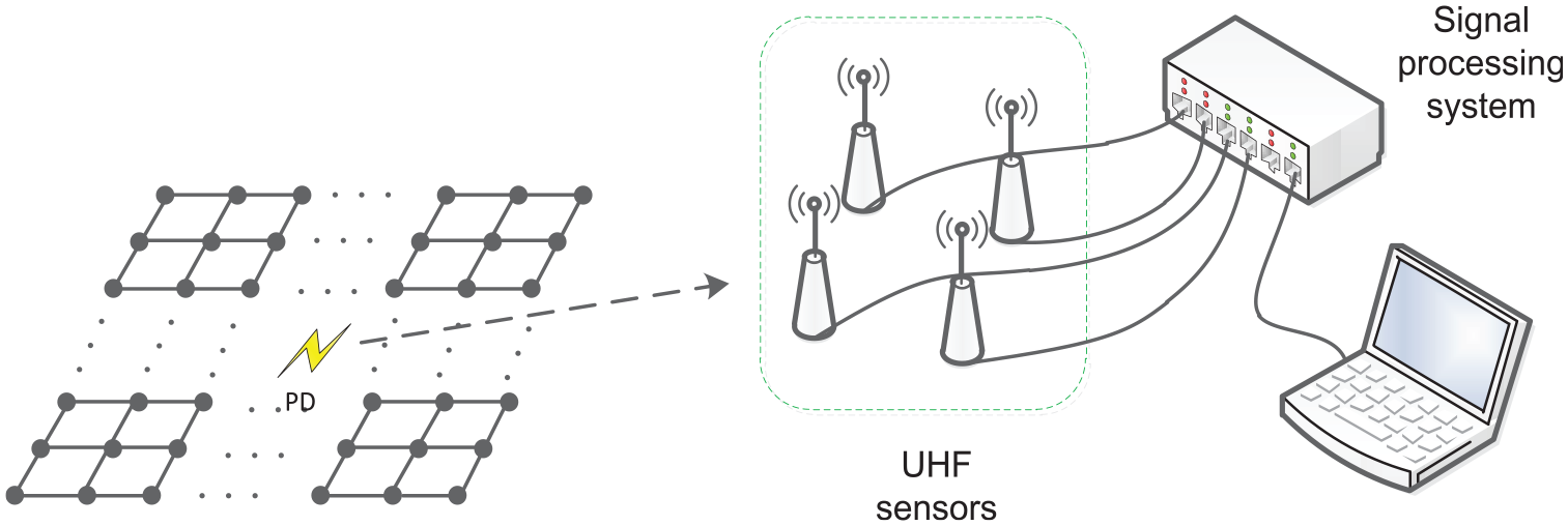
The key idea of the UHF method is to use very sensitive sensors. In many countries, sensors are typically installed in GIS. In China, however, external antennas are used. Because external antennas are used to detect the weak electromagnetic waves from PDs that leak from the insulation gap of the GIS, the signal is weak and needs to be filtered using a suitable algorithm. The principle of PD location with UHF sensors is based on the time and distance information that is available after the arrival of the electromagnetic wave (Figure 1). The corresponding calculation methods mainly consist of a search algorithm and an iteration algorithm. At the core of Newton’s iteration algorithm is the convergence of the computation. Relevant research includes the Taylor genetic algorithm proposed by Tang Ju of Chongqing University, the spatial search algorithm based on energy accumulation proposed by Gao Wensheng of Tsinghua University, and the global search iteration algorithm proposed by Tang Zhiguo of North China Electric Power University. 15 The search algorithm divides the detected object into several regions. It then uses the distance difference between the sensor and each region as the basis for the decision mode. If the standard mode corresponding to an area is the same as the decision mode, the area is identified as having a fault. Hasan Reza Mirzaei et al. 16 proposed a particle swarm optimization (PSO) algorithm by artificially modifying the standard pattern of the search algorithm. Lao Fangcheng, Zhang Xiaoxing, and Wang Hui 17 used a back propagation (BP) algorithm, a genetic algorithm, and a Gustafson–Kessel (GK) fuzzy classification algorithm to extract highly nonlinear spatial features to identify the discharge model. The results show that both their recognition ratio and robustness are good. Xu Di et al. 18 improved a received signal strength indicator (RSSI) ranging algorithm. Li Zhen et al. proposed RSSI localization based on compressed sensing, RSSI fingerprinting localization, and a localization method based on a UHF wireless sensor and a pattern recognition algorithm. All of these features improved the positioning accuracy.18–22 The main problems of RSSI ranging algorithms are that the ranging error is large, and the positioning accuracy for the nodes is biased. The error for the RSSI ranging algorithm was optimized using a PSO algorithm, which improved the positioning accuracy significantly.
Conventional location technique for a partial discharge source in TDOS switchgear.
Although time difference positioning is more accurate, the hardware requirements for the measuring equipment are also higher. In other words, high-precision measuring equipment is needed to determine the starting time of the UHF signal. This means that the method is both complex and costly. For the positioning calculation, the arrival time or time difference for the first wave causes errors. This may require an iterative algorithm, and it may be unable to converge locally. Compared to time difference location, RSSI location is less expensive, easier to implement, and has technical advantages.23,24
While RSSI-based positioning is usually based on the signal transmission model, the electromagnetic and spatial environment of a switchgear cabinet is complex, and applying the model can be difficult. Therefore, a wireless sensor array positioning method based on RSSI ranging that can locate PDs is proposed (Figure 2).

Partial discharge source location method for switchgear using RSSI ranging.
Even though RSSI ranging has low ranging accuracy, it does not require additional hardware. To overcome the complications due to the RSSI ranging error, it is necessary to use a position estimation algorithm with high estimation accuracy for the node location. This way, it is possible to estimate and improve the overall positioning accuracy of the positioning algorithm. 19 The PSO algorithm is a nearly ideal position estimation algorithm. It is very accurate but also has a problem with particle diversity. It can easily converge to a local optimal solution during the iteration, which reduces optimization accuracy. Therefore, a difference equation method is proposed to find the convergence conditions for the PSO algorithm. Subsequently, the PSO algorithm is applied with the convergence condition. After implementing these improvements, combined with the PSO algorithm to optimize the location of unknown nodes, it is possible to optimize the initial search space for the PSO. Furthermore, using simulation experiments, the effectiveness of the improved PSO algorithm and its application in UHF wireless sensor array positioning are verified.
Application of RSSI ranging for PD location
The localization algorithm that uses RSSI ranging consists of three steps. The first step is the ranging step, which uses RSSI ranging to obtain the distance between the local discharge source and the known nodes within the surrounding one-hop communication range. The second step is the location estimation step, which uses distance information to estimate the location of the unknown nodes. The last step is the location implementation step, which uses the position estimation algorithm to estimate the location of the unknown nodes. The results of the first two steps are used to locate unknown nodes of the UHF sensor array as accurately as possible.
Ranging with RSSI
In RSSI positioning, when the receiving node receives an electromagnetic wave signal from the PD source, the power at the receiving node can calculated from the RSSI register in the radio frequency (RF) chip. Because the transmission power of the transmitting node is known, the power loss of the radio wave during propagation can be calculated. Then, the distance between the receiving node and the transmitting node can be derived using the radio wave propagation loss model. Using the ideal free-space propagation model, the relationship between power loss and distance is
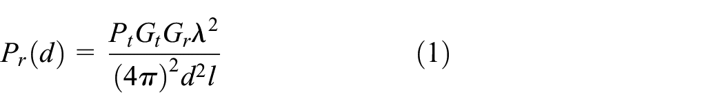
where
The equation shows that the propagation loss of the radio wave is inversely proportional to the square of the distance between the transmitting and receiving nodes. However, in practice, UHF sensors are used in relatively harsh environments, which means that there are many problems such as multipath fading, antenna gain reduction, and blocking by obstacles, which cause interference and loss of wireless signals. UHF sensors are often used in practice, and the following equation, which is based on the normal distribution model, can be applied to them
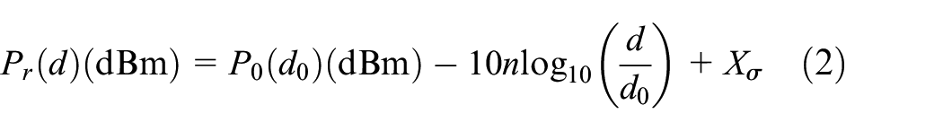
In equation (2),
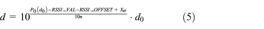
By solving for the distance d, the following equation can be obtained

The RF chip in the node provides a register to calculate the received power. The value of the register is recorded. The RF chip is updated every time it receives a data frame, and the received power of the RF chip is calculated using

Equation (4) represents an offset, usually provided by the RF chip supplier, from which the distance between the transmitter and the receiver can be derived using
Generally, the values of n and σ for a given environment need to be determined through many experiments. This way, RSSI can be measured accurately. The values of Li et al.
20
were obtained through a precise measurement:
Estimating an unknown node location
After using RSSI location to measure the distance between the location of the PD source and the known node in the range of one-hop communication, the position of the unknown node can be estimated with a position estimation algorithm. The location of the PD source is set as D, and its coordinates are (x, y). The number of known nodes in the range of the one-hop communication, measured through RSSI ranging, is n (where n ≥ 3), which is recorded as
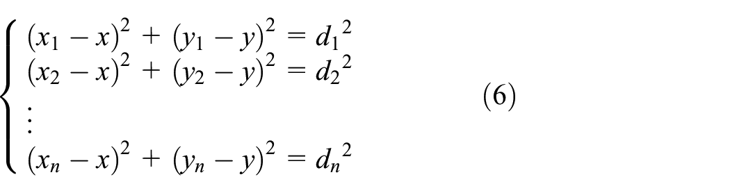
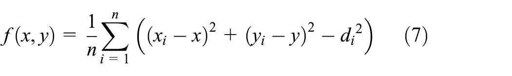
Equation (6) can be solved using a position estimation algorithm, such as the maximum likelihood estimation (MLE), to estimate the coordinates of D. Furthermore,

However, the estimation accuracy of the MLE is not high. Compared to other common ranging methods, the RSSI’s greatest weakness is that the ranging accuracy is not high. Therefore, it is desirable to find a more accurate estimation algorithm in our effort to improve the final positioning accuracy. Equation (6) can be seen as an extremum optimization problem, which means we aim to find coordinates
The PSO algorithm is simple in structure, easy to implement, does not require adjustment of many parameters, the time and space complexity of the algorithm is relatively low, and it can find a better optimized solution using less calculation power. Different individuals in PSO find the optimal solution for the complex space problem by information sharing, cooperation, and through several population iterations. Therefore, the PSO algorithm is used as the location estimation algorithm for unknown nodes to enable the localization of PD within the UHF sensor array.
Principle and process of PSO
PSO simulates the foraging process of birds in multidimensional space to solve the objective optimization problem. 21 For the optimization algorithm, each particle represents a bird which conducts a search for the objective optimization problem. The food that the birds want to find is the optimal value of the objective optimization problem.
Assuming that the particle number of particles in the swarm is N, and the dimension of each particle is D, that is, the group consists of N particle searches in D-dimensional space. Then, the coordinates of each particle can be expressed as

The velocity, corresponding to each particle, can be expressed as

The location of the historical optimum for each particle searched is expressed as

The location of the global historical optimum obtained by all particle searches is expressed as

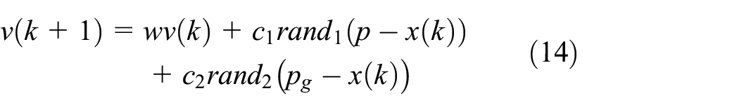
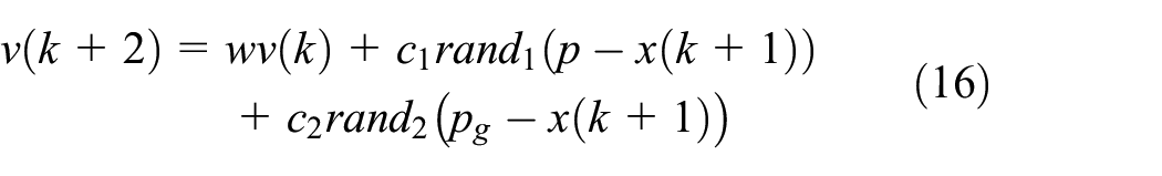
Then, in the (k + 1) iteration, the position and velocity update equation of the PSO is


Equations (12) and (13) are the speed and position update equations of the basic PSO algorithm, in which
A flowchart of the basic PSO algorithm is shown in Figure 3.
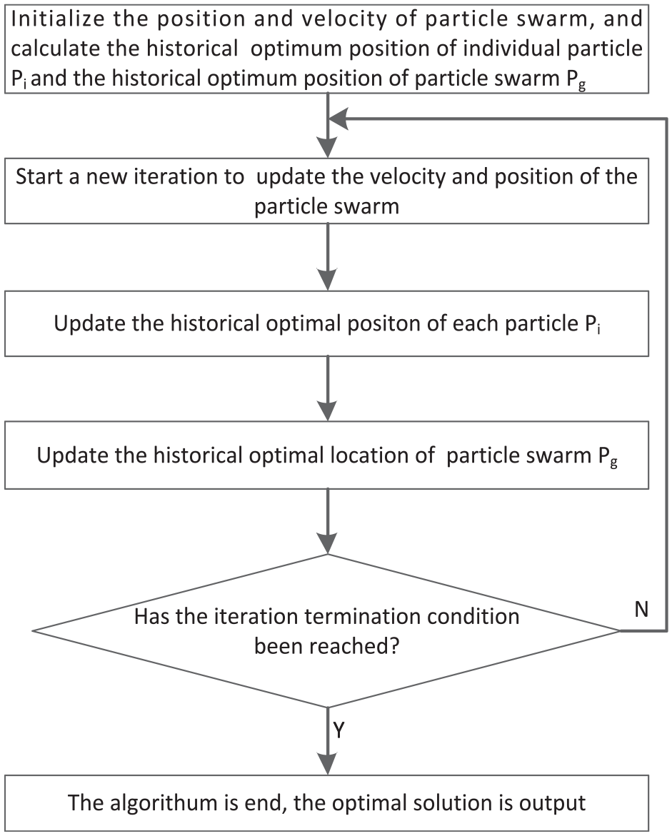
Flowchart for basic PSO.
Improved PSO algorithm for RSSI location optimization
Convergence analysis of the PSO algorithm
To ensure the effectiveness of the improved PSO algorithm, it is necessary to clarify its constraints with respect to algorithm improvement. Therefore, the convergence of the improved PSO algorithm was analyzed using the difference equation. Two simplifications were performed before the convergence of the improved PSO algorithm was analyzed. First, although the PSO algorithm searches in multidimensional space, each improved PSO algorithm was simplified as a result of the search process. Because the dimensions are completely independent of each other, the algorithm can be simplified to one dimension for analysis. Second, the individual historical optimal solution and the historical optimal solution of the particle population change substantially at the beginning of the search. However, after increasing the iterations, the two optimal solutions become (gradually) more stable. Therefore, to simplify the convergence analysis, it can be assumed that the location of the individual historical optimal solution, found by both particle and whole population, is unchanged; these are noted as p and pg, respectively. Based on the above two simplifications, equations (12) and (13) can be written using inertia weight

Using equations (14) and (15), this yields

Equations (15) and (16) are substituted into the equation (17) to obtain

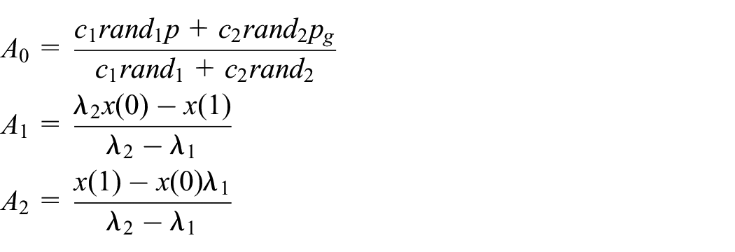
Equation (19) is a second-order nonhomogeneous difference equation with constant coefficients. Solving the difference equation, it is possible to obtain the relationship between x(k) and the initial conditions. The eigenvalue equation method is used to solve the equation.
The characteristic equation for equation (19) is

The two eigenvalues of the characteristic equation are


Let
If

where

2. If

where
3. If

where

Equations (22), (23), and (24) can be expressed in triangular form
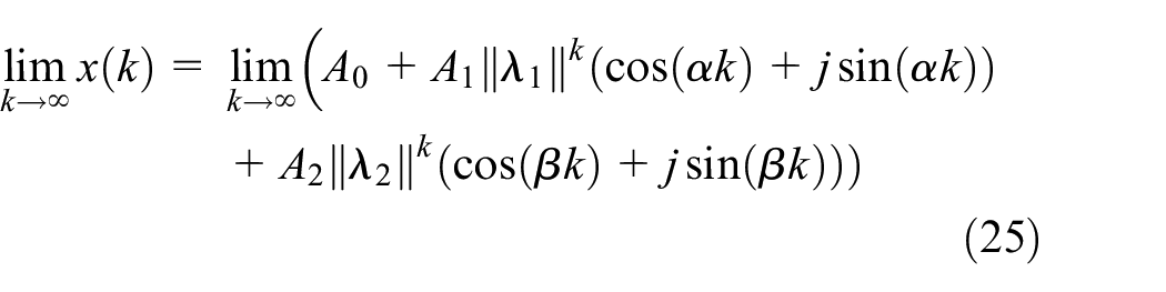
where
Take the limit of k in equation (25), it can be written as

Hence, if the PSO algorithm is converged, there must be
If

the PSO converges.
2. If

the PSO converges.
3. If
(a) When

the PSO converges.
(b) When

the PSO converges.
(c) When

the PSO converges.
According to Jiang, 14 if the PSO can converge to the global optimal solution with a larger probability, w > 0 is necessary. By synthesizing the conditions discussed above, it can be concluded that, if the PSO algorithm is to converge, the parameters of the algorithm need to satisfy the following conditions

Adaptive inertial weight PSO
The purpose of this article is to find an improved PSO algorithm, which can improve the convergence speed, escape the local optimum, and still maintain the characteristics of the original PSO algorithm: simple structure, easy implementation, and few adjustable parameters. The improved algorithm does not increase the time and space complexity of the algorithm, which means that it can be used for the localization of PD sources using UHF sensor arrays effectively.
Because inertia weight represents a key balance factor between global search and local search, 15 an self-adaptive particle swarn optimization (SAPSO) is proposed, which satisfies the above requirements.It has also been successfully used for the location of binary wireless sensor networks. In this algorithm, the inertia weight is determined by each particle’s own fitness value rather than the current iteration number. Assuming that the algorithm reveals an optimal minimum, the inertia weight can be calculated as follows
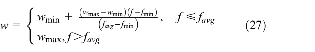
where
Improved learning factor PSO algorithms and processes based on adaptive inertial weight
Using the adaptive weighted particle swarm optimization (AWPSO), the parameters for the learning factors are further optimized to improve the optimization of the algorithm. To increase the uniformity of the iteration process, the learning factor is treated as a function of inertia weight. For particles with poor fitness, the self-learning ability is stronger, while the social learning ability is weaker, and the global search ability is improved to facilitate fast search. For particles with better fitness, the social learning ability is stronger, while the self-learning ability is weaker, and they have stronger locality. The fine search ability can help it converge toward the global optimal solution with high accuracy.
Given the constraints of the convergence condition equation (27) of the PSO, the parameters of cognitive factors c1 are modified as follows

According to equation (27), the inertia weight of the PSO is between (0, 1) assuming convergence. Therefore, within this interval, and for particles with poor fitness, w is larger and the corresponding
For the social factor

The flowchart for the improved learning factor PSO algorithm, based on adaptive inertia weight, is as follows:
Step 1: particle swarm with N and the number of dimension D is initialized. The initial velocity and position of the particles are set uniformly and randomly within the range for both velocity and position. The optimum individual position

Step 2: starting iteration k, the velocity of each particle is updated according to equation (10) with inertia weight, where the inertia weight is derived using equation (27) and the cognitive factor
Step 3: calculate the fitness for the current position of each particle
Step 4: for each particle, the fitness value of its current position is compared with that of its historical optimum position
Step 5: for each particle, the fitness of its current historical optimal position
Step 6: checking termination conditions. Generally, in this step, we decide whether the fitness value of
Experimental verification
Location procedure of the UHF sensor array using RSSI
A high-voltage hall was selected for the experiment in the field test area because the electromagnetic and space environments are complex and suitable to simulate a realistic environment for the switchgear. The main setup components were: (1) HZJF 10 kA/100 kV non-PD withstanding voltage test device; (2) HZJF-126 digital PD detector; (3) 220 V isolation filter; (4) YDTW-125/12 non-PD test transformer; (5) non-PD resistance; (6) 125 kV/550 pF non-PD capacitance divider; (7) CG3-12/140 type 120 pF capacitive sensor; (8) high-voltage lead for PD; (9) DK-34F1 multifunctional three-phase electrical measuring instrument calibration device; (10) TDS 1012B oscilloscope; (11) YDS996A function signal generator; (12) EMTEST mixed wave (surge) simulator UCS500N5V. Both hardware and software interfaces of the setup are shown in Figure 4. The data were obtained from the collection module of the interface of HZJF 10 kA/100 kV test device, and there were changed to the samples shown in Figure 6 using MATLAB.

Hardware and software interfaces of the test setup: (a) hardware equipment and (b) software interface.
Because the cabinet was 1.0 m × 2.2 m × 0.8 m, a measuring site, which was 2.2 m long and 3 m wide, was selected, as shown in Figure 5. The measurement points were arranged within a uniform grid, and a coordinate system was included in the plan. The positions of the four UHF sensors A1, A2, A3, and, A4 are shown in Figure 5. A total of 660 discharge waveforms were acquired by recording 10 sets of discharge waveforms received by four UHF sensors at each measurement point, using an analog PD source. Figure 6 shows the waveform of the PD signal, when the measurement point discharged at (2.0, 0.5).

Test area.
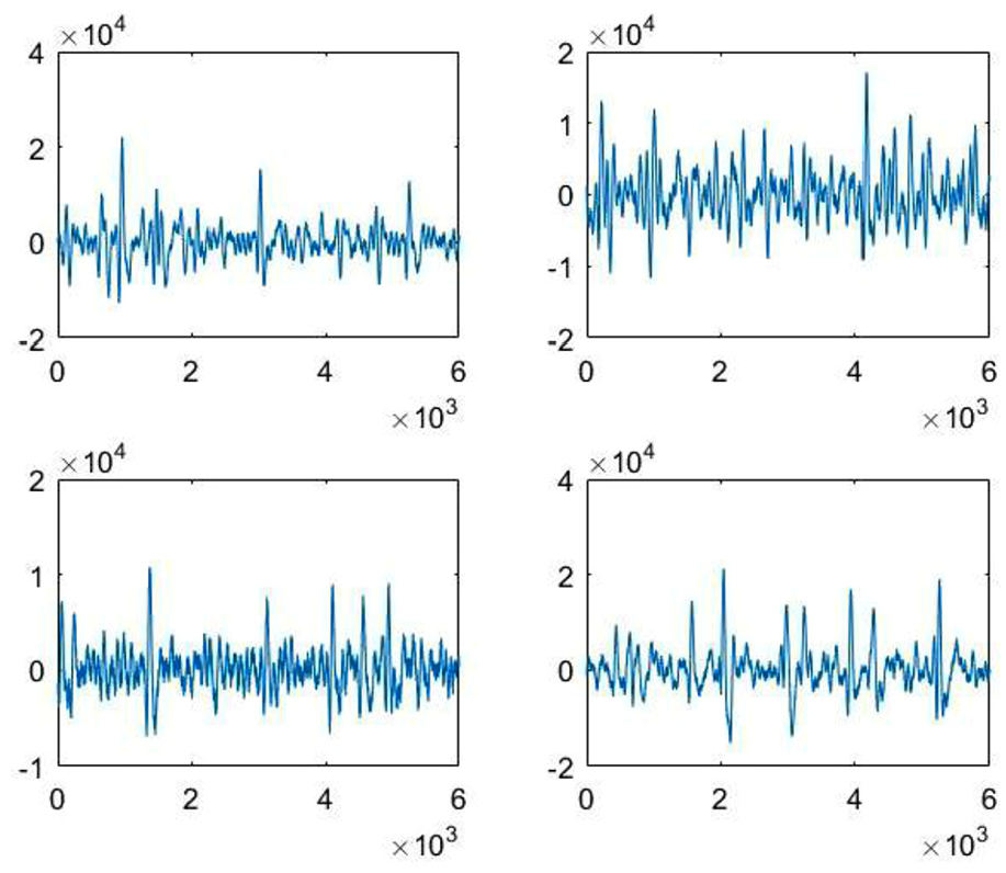
UHF waveform at one measurement point (2.0, 5.5).
After the UHF PD waveform received by the sensor was obtained, it was processed to determine the available RSSI value. The main steps of this process are: Gauss filtering, peak detection, and normalization.
During processing of the measured data, a Gauss filter was used to suppress the effect of interference pulses. The probability density function of the Gauss distribution can be written as

where x is a variable, and
After waveform filtering, the peak value of the measured waveform was extracted five times, and its mean was taken as the RSSI for the measured point. To overcome the effect of PD on the location, each RSSI value was normalized. There are four RSSI values at point Rj in Figure 4,

Normalization can highlight the relationship between the four RSSI values for each measurement point. It can also reduce the errors caused by the difference in intensity of the PD sources at different measurement points, and it can reduce the effect of any height change of the PD sources.
The UHF sensor array was placed in a specific area. When the positioning started, all beacon nodes sent their coordination data to all unknown nodes within the hop communication range and at a certain transmission power. The unknown node receives coordinate data from neighboring beacon nodes and reads the RSSI register value, which is recorded as RSSI_VAL. It also calculates the corresponding neighboring letter considering RSSI_VAL. The first step is to measure the distance between the benchmark nodes. After receiving and calculating all coordinate information, the PSO algorithm was used to estimate the position of each unknown node, whose distance exceeds three or more neighboring beacon nodes. This represents the second step (position estimation).
However, the location of the unknown nodes, whose number of neighbor beacon nodes was below three, could not be estimated at that time. Further processing was needed using the estimated coordinates of the unknown nodes, whose position was estimated to obtain the location of all unknown nodes (as far away as possible). This was the third step of the localization algorithm (location realization).
Parameter settings
To evaluate the performance of the improved algorithm in PD location, the improved SAPSO (ISAPSO) algorithms, PSO, and SAPSO were simulated using MATLAB, according to the positioning process described in the previous section.
The main parameters of the simulation experiment were: 66 nodes distributed within a 2.2 m long and 3 m wide two-dimensional (2D) region. The default value for the RSSI ranging maximum error was 20%, the size of the particle swarm was 20%, and the maximum iteration number of the particle swarm was 100. The PSO algorithm used
Experimental results and analysis
Using the simulation, the position estimation effect of the three PSO algorithms with respect to the effect of the RSSI ranging maximum error on positioning accuracy, as well as the processing time of the three PSO algorithms, was studied. To minimize all random errors, all tests were repeated 100 times under the same conditions.
Assuming that the number of unknown nodes to be located is N, the actual coordinates of the unknown node are

Relationship between the maximum error of RSSI ranging and the average positioning error
Figure 7 shows the variation of the average positioning error for the three PSO position estimation algorithms when the maximum error of RSSI ranging changes from 5% to 50%. When the maximum ranging error of RSSI increases, the average positioning error increases accordingly, but, compared with the PSO and SAPSO position estimation algorithms, the proposed ISAPSO algorithm still achieves the minimum average positioning error. This suggests that the ISAPSO algorithm proposed in this article achieves the best error minimization.
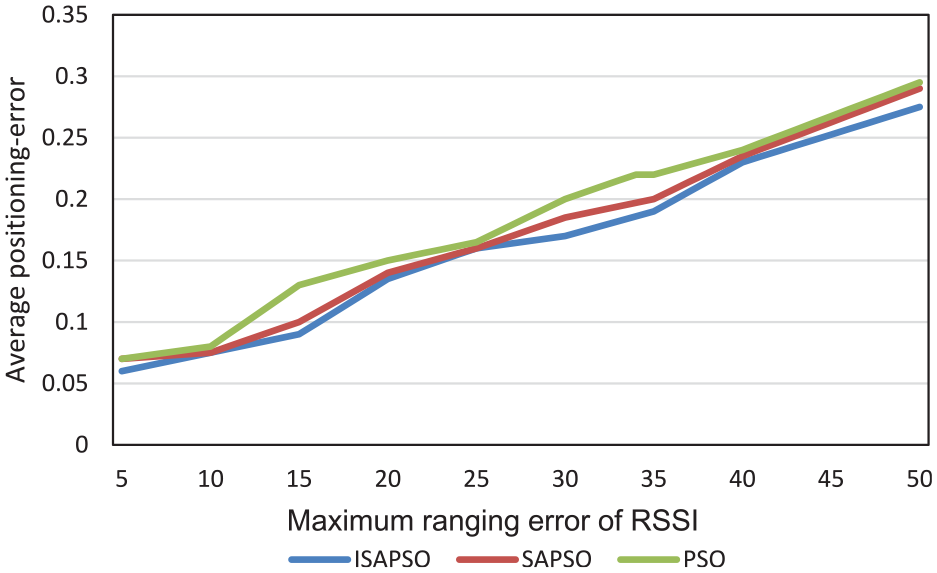
Relationship between RSSI maximum ranging error and average positioning error.
Real-time measurement and power consumption
The difference between real-time performance and power consumption is mainly reflected in the complexity of the algorithm, that is, the calculation time needed by the location estimation algorithm under the same conditions. The data in Table 1 show that the calculation time required by ISAPSO is very close to that of PSO and SAPSO under the same operating conditions. Therefore, the ISAPSO algorithm is close with respect to real-time performance and power consumption to both the PSO and SAPSO. It lists the average of the optimal values obtained by the three algorithms in 100 repeated experiments, and it shows the calculated standard deviation of the optimal values to observe the stability of the optimization effect. The smaller the standard deviation, the more stable is the performance of the algorithm. Both time and space complexity of the improved optimization algorithm proposed in this article do not increase.
Stability and required calculation times for the optimization of the three algorithms.

RSSI: received signal strength indicator; PSO: particle swarm optimization.
Table 1 shows the optimization performance of the three algorithms. It lists the averages of the optimal values obtained by the three algorithms in 100 repeated experiments, as well as the calculated standard deviation for the optimal values. This demonstrates the stability of the optimization effect. The smaller the standard deviation, the more stable is the algorithm. Our analysis indicates that the time and space complexities of the improved optimization algorithm do not increase.
To verify the performance of the improved algorithm for PD location, the measured RSSI values for PDs were input into the improved versions of ISAPSO, PSO, and SAPSO, respectively. In addition, the location results were recorded after 20 repeated calculations. The locations of 20 points are shown in Figure 8, and the three locations are shown in Table 2.

Simulation result of the improved ISAPSO algorithm.
Location results.

PSO: particle swarm optimization.
In conclusion, the positioning accuracy of the ISAPSO algorithm is better than the two other investigated algorithms, without increased time and space complexity. The positioning error of ISAPSO, with RSSI ranging, is 0.362 m. The ISAPSO algorithm also performs best for repeated calculations, which means, the location results are the most stable. In other words, the results confirm the accuracy and effectiveness of the PD algorithm with RSSI ranging.
Conclusion
Using RSSI location, in this study, we describe a novel and accurate location method for PD in switchgear for a UHF wireless sensor array. The benefits of the RSSI for realistic PD location in switchgear were analyzed. Then, taking into account the complex electromagnetic environment of switchgears, an improved PSO algorithm for PD location with RSSI ranging was proposed. Using a simulated PD signal to test the algorithm, the following conclusions were drawn
Because the attenuation of the ultrasonic signal is severe during propagation, the discharge source is undetectable, and the detection sensitivity is generally low. For this reason, UHF was used. A UHF wireless sensor with RSSI function does not require additional hardware, which makes the localization of PD sources easier. A significant drawback of RSSI ranging is that the ranging accuracy is not high. Therefore, it is necessary to use an algorithm with higher accuracy in the following location estimation algorithm to improve the final location algorithm of the UHF sensor array with RSSI ranging.
Unlike the original PSO algorithm, the improved ISAPSO algorithm does not increase the time and space complexity, instead it also tends to maintain the characteristics of the PSO algorithm, which are simple structure, easy implementation, and less adjustment of parameters required. The ISAPSO is improved according to the position of UHF sensor array. The simulation results also reveal that, compared with PSO and SAPSO algorithms, the ISAPSO achieves better optimization accuracy, while still maintaining the abovementioned advantages.
The location algorithm with a signal amplitude intensity distribution is more accurate and stable, and the positioning error of ISAPSO, with RSSI ranging, is 0.362 m. It is also more practical due to the less expensive hardware and software required.
Footnotes
Handling Editor: Xiangyang Xu
Declaration of conflicting interests
The author(s) declared no potential conflicts of interest with respect to the research, authorship, and/or publication of this article.
Funding
This work is supported by the Fundamental Research Funds for the Central Universities, No.2017B21214