Wireless sensor indoor positioning based on an improved particle filter algorithm

Abstract

Positioning by wireless sensor network is one of its main functions and has been widely used in many fields. However, when signal propagation is hindered, serious errors, non-line-of-sight errors, occur. In order to solve this problem, this article proposes an improved particle filter algorithm, which introduces the idea of residual analysis to improve reliability. The algorithm assigns weights to the particles based on the residuals and selects the appropriate particles. In addition, the non-line-of-sight error parameter $\alpha$ is introduced, and the second selection is made according to $\alpha$ , which considers the influence of non-line-of-sight error. The non-line-of-sight error is greatly reduced after two selections. The simulation is performed under several different non-line-of-sight errors, and results show that the algorithm is superior to Kalman filter and particle filter.

Introduction

Wireless sensor network (WSN) is a hot topic in recent years. By using sensors to collect data, it is easy to obtain various information of the monitored area. Positioning ¹ is one of its main functions and has been widely used in many fields. It uses two classes of nodes: fixed nodes and mobile nodes. The fixed nodes are distributed in the positioning area, the coordinates are known, and the mobile node is fixed on the positioning target.

Traditional methods have some errors in the actual situation: one is the measurement error, which is caused by system noise or measurement noise; the other is the non-line-of-sight (NLOS) error, which is the main challenge in positioning. It occurs when the signal propagation is hindered by some obstacles. In different scenarios, the NLOS error is subjected to different distribution functions. In order to minimize the impact of NLOS errors, some new algorithms have been proposed and they can be divided into two classes generally: one is to detect and select measurements which have no NLOS error. Shi et al. ² used channel visual information to improve positioning accuracy. A recurrent neural network was proposed in Choi et al. ³ ; it proposed a recurrent neural network (RNN) model, which takes a series of channel state information (CSI) to identify the corresponding channel condition. Based on distributed filter, a new NLOS recognition algorithm was proposed in Pak et al. ⁴ ; it proposes a new NLOS identification algorithm based on distributed filtering to mitigate NLOS effects, including localization failures. Momtaz et al. ⁵ proposed a new algorithm based on subspace method to identify and eliminate NLOS errors.

The other is weighting data with unknown propagation status. Tomic et al. ⁶ proposed a positioning method using received signal strength (RSS) and angle of arrival (AOA). The positioning problem was transformed into the framework of a generalized trust region sub-problem in Tomic and Beko. ⁷ Abu-Shaban et al. ⁸ proposed a closed estimator for locating mobile stations (MSs) through three base stations (BSs) in a cellular network. There was a two-stage closed-form estimator to localize an MS by three BSs in cellular networks. It used a distance-dependent bias model to derive a range estimator as a first step. Then it used trilateration to find an estimate of the MS position. Ding and Qi ⁹ proposed a new convex optimization model. Wang et al. ¹⁰ proposed a deviceless wireless sensing system based on multi-domain features. Wang et al. ¹¹ developed a new robust optimization method source location.

However, the first method will loose a lot of measurement data, resulting in lower positioning accuracy. The second method does not consider the signal propagation state, the weight does not reflect the actual situation well, and the adaptability of the algorithm is not strong. The article proposes an improved particle filter (IMPF) algorithm to solve these problems. The main innovation of the article lies in two points: it reduces the influence of NLOS error on positioning, and it has a great influence on the positioning accuracy, but there is no related paper to discuss it. All the sensors share the generated particles, so the computational complexity of the algorithm does not increase rapidly as the number of nodes increases. Different from traditional particle filter, in the article, some reasonable particles are selected to positioning by making two selections based on residual analysis. These particles will have weights based on the residuals. The selection reduces the influence of the NLOS error and the target is localized by the particles. The simulation is performed under several different NLOS errors, and results show that the algorithm is superior to Kalman filter (KF) and particle filter (PF).

Signal model

The propagation conditions of wireless communication systems are usually divided into two environments: line of sight (LOS) and non-line of sight (NLOS). In the case of obstacles, the wireless signal can only reach the receiving end through reflection, scattering, and diffraction, which we call NLOS communication. At this time, the wireless signal is received through multiple channels, and the multipath effect causes a series of problems such as delay in synchronization, signal attenuation, polarization change, and link instability, which are NLOS errors in Dou and Lei. ¹²

As shown in Figure 1, $N$ fixed nodes are randomly deployed in a certain scenario to locate a mobile node. The coordinate of the fixed node i is $[x_i,y_i](i=1,2,\dots ,N)$ and the mobile node is $[x,y]$ .

Figure 1.

Signal transmission model.

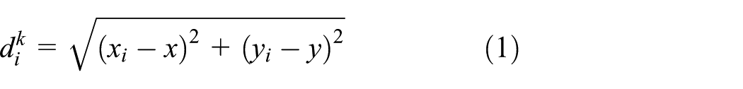
Ideally, the distance between the mobile node and the ith fixed node (i = 1, 2, …, N) at time k is defined by equation (1)

$$d_i^k=\sqrt{{(x_i-x)}^2+{(y_i-y)}^2}$$

(1)

However, there are some noises in practical applications, including system noise and measurement noise. In the LOS state, the measured distance is defined by equation (2)

$${\hat{d}}_i^k=\sqrt{{(x_i-x)}^2+{(y_i-y)}^2}+ϵ$$

(2)

where $ϵ$ is the measurement error, and it satisfies the Gaussian distribution and mean is 0. According to the existing research, estimating the measurement error distribution function as a Gaussian distribution function is an effective method. ¹³

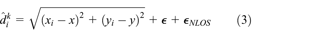
In addition, the direct path between the fixed node and the mobile node may be blocked by obstacles, as shown in Figure 1, and this propagation mode is NLOS. The signal can be diffraction, reflection, or refraction, and the distance will increase as shown in equation (3)

$${\hat{d}}_i^k=\sqrt{{(x_i-x)}^2+{(y_i-y)}^2}+ϵ+{ϵ}_{\mathrm{NLOS}}$$

(3)

where ${ϵ}_{\mathrm{NLOS}}$ is the NLOS error, and it has various distributions under various conditions.

• When it is a Gaussian distribution

$$f\left({ϵ}_{\mathrm{NLOS}}\right)=\frac{1}{\sqrt{2\pi {\sigma }_{\mathrm{NLOS}}^2}}\exp (-\frac{{({ϵ}_{\mathrm{NLOS}}-{\mu }_{\mathrm{NLOS}})}^2}{2{\sigma }_{\mathrm{NLOS}}^2})$$

(4)

where ${\sigma }_{\mathrm{NLOS}}$ is the standard deviation of the function and ${\mu }_{\mathrm{NLOS}}$ is the expectation of the function.

• When it is uniform distribution ${ϵ}_{\mathrm{NLOS}}(u_{\min },u_{\max })$

$$f\left({ϵ}_{\mathrm{NLOS}}\right)=\{\begin{array}{cc}\frac{1}{u_{\max }-u_{\min }}\hfill & \begin{array}{c}{u}_{\min }\le {ϵ}_{\mathrm{NLOS}}\le u_{\max }\hfill \\ \multicolumn{1}{c}{\mathrm{else}}\end{array}\hfill \\ \multicolumn{1}{c}{0}& \hfill \end{array}$$

(5)

where $u_{\min }$ and $u_{\max }$ are the upper and lower boundaries of the distribution, respectively. The variable is evently distributed from $u_{\min }$ to $u_{\max }$ .

• When it is exponential distribution ${ϵ}_{\mathrm{NLOS}}(\lambda )$

$$f\left({ϵ}_{\mathrm{NLOS}}\right)=\{\begin{array}{cc}{\lambda }^{-1}\exp \left(\frac{-{ϵ}_{\mathrm{NLOS}}}{\lambda }\right)\hfill & {ϵ}_{\mathrm{NLOS}}\ge 0\hfill \\ \multicolumn{1}{c}{0}& {ϵ}_{\mathrm{NLOS}}<0\hfill \end{array}$$

(6)

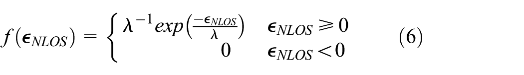
where $\lambda$ is rate parameter, and it is the number of times an event occurred per unit of time.

IMPF algorithm

Particle filter

The PF is developed in the late 1990s. It is another form of implementation of recursive Bayesian filtering. ¹⁴ It uses a set of particles (also called samples) to represent the posterior distribution of some stochastic process given noisy and/or partial observations. The state-space model can be nonlinear, and the initial state and noise distributions can take any form required. PF techniques provide a well-established methodology.^15–17

There are many studies about it in positioning systems. A new fusion-simulated multi-feature-based improved simulated annealing PF tracking algorithm is proposed in Zhao et al. ¹⁸ Li and Liu ¹⁹ proposed a new PF algorithm that combines the traditional PF algorithm with the KF algorithm. Liu ²⁰ proposed a Gaussian and PF pre-detection tracking algorithm called the Gaussian sum particle filter–track before detect (GSPF-TBD) algorithm.

Parameter description

Suppose there are P particles and N fixed nodes. At time k, the measured distance between the mobile node and the ith fixed node is ${\hat{d}}_i^k$ , the distance between the pth particle and the ith fixed node is ${\hat{d}}_{i,p}^k$ , the weight is given based on the distance difference, and it is $W_{i,p}^k$ . The flow chart of the algorithm is shown in Figure 2.

Figure 2.

Description of the experimental scenario.

Particle weighting

The particle weight is related to the positioning result. Unlike general PF, IMPF obtains particle weight by residual analysis rather than Gaussian function. The whole process is implemented as follows:

• Calculate the distance ${\hat{d}}_{i,p}^k$ and ${\hat{d}}_i^k$ . Define the difference as the residual of pth particle to ith fixed node, denoted as ${\mathrm{res}}_{i,p}^k$

$${\mathrm{res}}_{i,p}^k=|{\hat{d}}_{i,p}^k-{\hat{d}}_i^k|$$

(7)

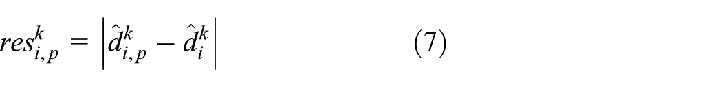
• Calculate the residuals of the pth particles of each fixed node and add them together. Define it as the residual of pth particle, denoted as ${\mathrm{res}}_p^k$

$${\mathrm{res}}_{i,p}^k=\sum _{i=1}^N|{\hat{d}}_{i,p}^k-{\hat{d}}_i^k|$$

(8)

• Find the reciprocal of ${\mathrm{res}}_p^k$ , and it is the weight of the pth particle

$$W_p^k=\frac{1}{{\mathrm{res}}_{i,p}^k}$$

(9)

Particle selection

First selection

When all the particle weights are obtained, it will make the first selection. As the weight indicates the possibility that the particle is suitable for mobile node, first selection chooses some particles with larger weights and defines the average weight as threshold. Given the generated P particles and their weights W, first selection will choose S particles from them.

First selection chooses some particles with larger weights, which are reasonable at the overall level. However, once there are several fixed nodes that are inaccurate in determining the particles, some unreasonable particles can also pass first selection. Therefore, a second selection is necessary.

Second selection

The probability of NLOS errors can be estimated using particle residuals. It is assumed that the state where the residual is greater than the average contains the NLOS error. The residual ratio that is considered to contain the NLOS error is recorded as $\lambda$ . Therefore, for the LOS propagation, there are approximately N(1 – λ) fixed nodes whose residuals are less than the residual mean. When a particle is away from the mobile node, its residual will also become larger. The particles with greater residuals will be discarded.

The particle number will be checked before positioning begins. When the propagation state is terrible, most propagation between the fixed node and the mobile node have NLOS errors, and when no particles are left after selections for the contradiction, then particles selected in first selection are used; otherwise, those that are selected in second selection are used. See Table 1 for fake code of related algorithm.

Table 1.

Alogrithm second selection.

Input: $S$ particles with weights $W_i^k(i=1,2,\dots ,S)$

Output: $Q$ particles with weights $W_i^k(i=1,2,\dots ,Q)$

1. $a=0$

2. for $i=1:N$

3.  for $j=1:S$

4.   if ${\mathrm{res}}_{i,j}^k\ge \sum _{p=1}^S\frac{{\mathrm{res}}_p^k}{(S\times N)}$

5.    a = a + 1

6.  end for

7. end for

8. $\lambda =\frac{a}{S\times N}$

9. $t=N\times (1-\lambda )$

10. for $j=1:S$

11.  $b=0$

12.  for $i=1:N$

13.   if ${\mathrm{res}}_{i,j}^k\le \sum _{p=1}^S\frac{{\mathrm{res}}_p^k}{S\times N}$

14.    b = b + 1

15.  end for

16.  if $b>t$

17.   particle reserved

18.  else

19.   particle discard

20. end for

Location estimate

Least squares method

It is a mathematical optimization method. It finds the best function match for the data by minimizing the sum of the squares of the errors. A typical class of functional models is the linear function model. Location estimate algorithm is based on linear least squares (LLS).

Consider the overdetermined equations $\sum _{j=1}^n{X}_{\mathrm{ij}}{\beta }_j=y_i,(i=1,2,3,\dots ,m)$ , where m represents m equations and n represents n unknowns $\beta$ . After it is vectorized, it is $X\beta =y$ , and the equations generally have no solution; so in order to select the most appropriate $\beta$ to make the equation as far as possible, the residual sum-of-squares function $S(\beta )=||X\beta -y|{|}^2$ is introduced. When $\beta =\hat{\beta },S(\beta )$ is the minimum, $\hat{\beta }=\mathrm{argmin}(S(\beta ))$ . Derivating $S(\beta )$ and finding the extreme value, we can get $X^{T}X\hat{\beta }=X^{T}y$ , and if $X^{T}X$ is a non-singular matrix, $\beta =(X^{T}X{)}^{-1}{X}^{T}y$ is a unique solution.

Location estimate

Assuming that first selection chooses S particles and second selection chooses Q particles, and the retained particle number $L=S$ when a contradiction occurs, otherwise $L=Q$ .

Before the positioning begins, the retained particle weights will be normalized, and the weight of pth particle at time k is denoted as ${\mathrm{NW}}_p^k$ . At time k, for the ith fixed node, the distance ${\mathrm{dis}}_i^k$ between it and the mobile node can be given by

$${\mathrm{dis}}_i^k=\sum _{p=1}^L{\mathrm{NW}}_p^k{\hat{d}}_{i,p}^k$$

(10)

We can get the distance $(\mathrm{di}{s}_i)$ at time $k$ and other times by equation (10). When all $\mathrm{dis}$ are known, as all coordinates of fixed nodes are known in advance, the ones of the mobile node can be calculated. They are obtained using the maximum likelihood, and it can be explained by the following equation. First, according to the coordinates of the mobile node and the fixed node, the distance between them is defined as equation (11)

$$\{\begin{array}{c}{(x_1-x)}^2+{(y_1-y)}^2={\left(\mathrm{di}{s}_1\right)}^2\hfill \\ \multicolumn{1}{c}{⋮}\\ \multicolumn{1}{c}{{(x_N-x)}^2+{(y_N-y)}^2={\left(\mathrm{di}{s}_N\right)}^2}\end{array}$$

(11)

Then by calculating equation (11), we get equation (12)

$$\{\begin{array}{c}2x(x_1-x_2)+2y(y_1-y_2)\hfill \\ \multicolumn{1}{c}{={\left(\mathrm{di}{s}_2\right)}^2-{\left(\mathrm{di}{s}_1\right)}^2-(x_2^2+y_2^2)+(x_1^2+y_1^2)}\\ \multicolumn{1}{c}{⋮}\\ \multicolumn{1}{c}{2x(x_1-x_N)+2y(y_1-y_N)}\\ \multicolumn{1}{c}{={\left(\mathrm{di}{s}_N\right)}^2-{\left(\mathrm{di}{s}_1\right)}^2-(x_N^2+y_N^2)+(x_1^2+y_1^2)}\end{array}$$

(12)

The above equations can be expressed by the linear equation AX = B, where A and B are defined as equation (13)

$$\begin{array}{cc}A\hfill & =\left[\begin{array}{cc}(x_1-x_2)\hfill & (y_1-y_2)\hfill \\ \multicolumn{1}{c}{(x_1-x_3)}& (y_1-y_3)\hfill \\ \multicolumn{1}{c}{⋮}& ⋮\hfill \\ \multicolumn{1}{c}{(x_1-y_N)}& (y_1-y_N)\hfill \end{array}\right]\hfill \\ \multicolumn{1}{c}{B}& =\left[\begin{array}{c}{\left(\mathrm{di}{s}_2\right)}^2-{\left(\mathrm{di}{s}_1\right)}^2-(x_2^2+y_2^2)+(x_1^2+y_1^2)\hfill \\ \multicolumn{1}{c}{{\left(\mathrm{di}{s}_3\right)}^2-{\left(\mathrm{di}{s}_1\right)}^2-(x_3^2+y_3^2)+(x_1^2+y_1^2)}\\ \multicolumn{1}{c}{⋮}\\ \multicolumn{1}{c}{{\left(\mathrm{di}{s}_N\right)}^2-{\left(\mathrm{di}{s}_1\right)}^2-(x_N^2+y_N^2)+(x_1^2+y_1^2)}\end{array}\right]\hfill \end{array}$$

(13)

Finally, the estimated coordinates of the mobile node is

$${[x,y]}^T={\left(A^{T}A\right)}^{-1}{A}^{T}B$$

(14)

Particle replication and motion

Once the positioning is complete, the retained particles will be utilized for next positioning. Therefore, construct replication layer to determine the particle replication process. The length of every layer is the weight of the particles. As the normalization of weights, the total length of all layers is 1. When constructing a layer, a random number satisfying uniform distribution from 0 to 1 is generated. Random numbers fall into some layer, and the corresponding particles are copied once. It can ensure that particles with larger weights have more chances to replicate while avoiding local optimization.

After the copying process is completed, the new particles will be distributed in a small range, avoiding excessive concentration of the particles. The variance of the coordinate obeys a Gaussian distribution with a mean of 0 and a variance ${\sigma }_p^2$ . These particles will be utilized for next positioning. The motion of the particle is given by equation (15)

$$(X_p^{k+1},Y_p^{k+1})=(X_p^k,Y_p^k)+N(0,{\sigma }_p^2)$$

(15)

Simulation

The simulation runs on MATLAB, which evaluates the performance of the algorithm and compares it to the KF and the PF. The position of each Monte Carlo-operated fixed node is evenly deployed in a space of 100 × 100 m². Root mean square error (RMSE) as an indicator, defined by equation (16)

$$\mathrm{RMSE}={(\frac{1}{K{t}_n}\sum _{i=1}^{t_n}\sum _{k=1}^K{(x(k)-{\hat{x}}_i(k))}^2+{(y(k)-{\hat{y}}_i(k))}^2)}^{\frac{1}{2}}$$

(16)

where $t_n=1000$ , $K=100$ , $[x(k),y(k)]$ is the actual coordinate at time k, and $[{\hat{x}}_i(k),{\hat{y}}_i(k)]$ is the estimate of the ith time. Simulation is performed under NLOS error obeying different distribution functions. The simulation will verify the superiority of this new idea compared to particle filtering and Kalman filtering, which will serve as the basis for future work.

NLOS error obeys the Gaussian distribution

Figure 3 shows the positioning results of IMPF. Even if the fixed nodes are randomly deployed, in most cases, the estimated value of the algorithm is very close to the true value. When a step has large error, such as x = 80, it can also be corrected quickly, and a reasonable positioning result can be obtained without error accumulation leading to positioning failure.

Figure 3.

IMPF positioning simulation results in 100 × 100 m².

Figure 4 shows the cumulative distribution function (CDF) of the positioning error. It can be seen that the average positioning error of IMPF is about 2.5 m and that of KF and PF is about 4 m. The error of 90% in IMPF is less than 6.2 m, that is, under the given conditions, IMPF can basically control the error within 6 m, while that of PF is 10 m, KF exceeds 10 m. The positioning accuracies are obviously different. There is a cross point between the curves of PF and KF, probably due to particle distribution. Because some particles will deviate from the target, the PF curve is lower than the KF curve, but most of the particles are distributed near the target. In addition, KF is more susceptible to NLOS, which may also be the reason of the cross point.

Figure 4.

The trend of CDF with increasing positioning errors.

${\sigma }_i$ is the standard deviation of the measured noise, and Figure 5 shows how it affects the positioning error. It changes from 1 to 7, which means when there is more measured noise, the RMSE of all algorithms increases. Under different ${\sigma }_i$ , the performance of IMPF is always better than the other algorithms. Specifically, compared with the PF and KF, the positioning accuracy of IMPF improves by 11.9% and 17.8%.

Figure 5.

The trend of RMSE with ${\sigma }_i$ under the Gaussian distribution.

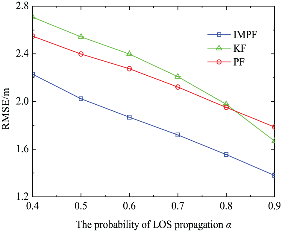
Figure 6 shows the effect of the number of fixed nodes on the positioning error. With the increase in the number of fixed nodes, IMPF algorithm has better positioning results than KF and PF. As the number of fixed nodes increases, more fixed nodes are again in LOS conditions where KF will get a better localization result than PF. When the number of fixed nodes is 5, compared with PF and KF, the positioning accuracy of IMPF improves by 15.4% and 23.3%, and the fixed nodes continue to increase, and this number will also increase.

Figure 6.

The trend of RMSE with the number of increasing fixed nodes.

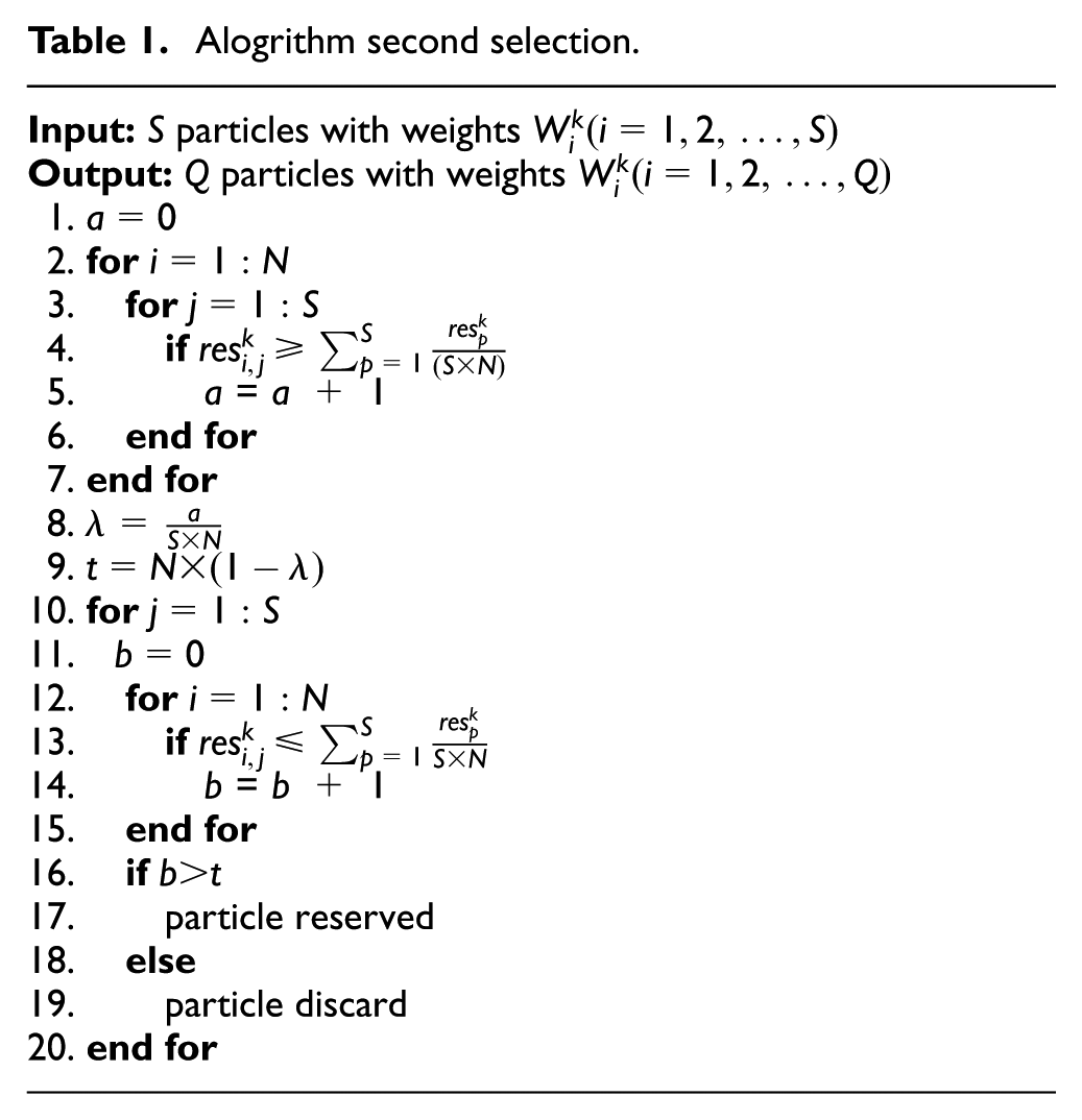
Figure 7 shows that the positioning errors increase with NLOS error. In Figure 7(a), the average of RMSE in IMPF is 2.024 m, but it is 2.554 and 2.379 m in KF and PF, respectively. The RMSE difference of the three algorithms remains basically unchanged. In Figure 7(b), the RMSE of IMPF increases slower than that of KF, and the larger the standard deviation, the more obvious the advantage of IMPF. When the standard deviation is 9, the positioning accuracy of IMPF is 25.1% higher than KF and 15.3% higher than PF.

Figure 7.

The trend of RMSE with increasing NLOS errors: (a) mean of NLOS error and (b) standard deviation of NLOS error.

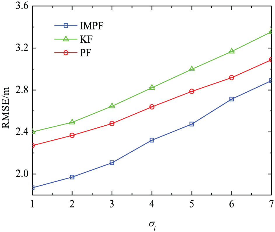
Figure 8 shows the effect of LOS propagation probability $\alpha$ on positioning error. It can be seen that the positioning error decreases as the value of $\alpha$ increases. This is because the larger the $\alpha$ , the more the fixed nodes in the LOS state, and the smaller the NLOS interference. It confirms the result in Figure 6. The downward trend of the three algorithms is roughly equivalent. Compared with PF and KF, the positioning accuracy of IMPF is improved by 17.4% and 20.1%. Combined with Figures 8 and 9, it can be seen that NLOS has a great influence on the positioning error, and the IMPF algorithm is significantly better than the popular KF and PF algorithms for NLOS.

Figure 8.

The trend of RMSE with increasing $\alpha$ .

Figure 9.

The CDF of positioning errors.

NLOS error obeys uniform distribution

Figure 9 shows the CDF of the positioning error. The average positioning error of the IMPF is about 3.75 m. In the same case, the average error of KF and PF is about 5 m. IMPF achieves the lowest positioning error.The positioning error of the algorithm in Figure 10 is similar to that in Figure 6. It can be seen that the positioning error of IMPF is about 0.4 m lower than that of KF and about 0.1 m lower than that of PF. Compared with PF and KF, the positioning accuracy of IMPF is increased by 5.7% and 10.8%, respectively.

Figure 10.

The trend of RMSE with ${\sigma }_i$ under the uniform distribution.

Figure 11 shows that RMSEs decline with more fixed nodes. The more fixed nodes are deployed, the less positioning errors are obtained, which is the same as Figure 7. KF and IMPF are greatly affected by the number of fixed nodes. When the number of fixed nodes increases, the positioning error will decrease rapidly. The performance of KF will exceed that of PF for the same reason in Figure 6. IMPF always maintains the lowest error throughout the change. When the number of fixed nodes is 10, the positioning accuracy of IMPF is improved by 12.7% compared with KF and 12.6% compared with PF.

Figure 11.

The trend of RMSE with the number of increasing fixed nodes.

The effect of the parameter $U_{\max }$ on the positioning error is shown in Figure 12. As $U_{\max }$ increases, the performance of algorithms decreases. IMPF maintains the best positioning result, which is about 0.2 m lower than the positioning error of PF, and the difference with KF increases as $U_{\max }$ increases. With the increasing $U_{\max }$ , NLOS error distribution will be more uniform, which means more fixed nodes in NLOS. So the curve of PF is little lower than the curve of KF. Compared with KF and PF, its positioning accuracy increases by 10.3% and 9.0% on average.

Figure 12.

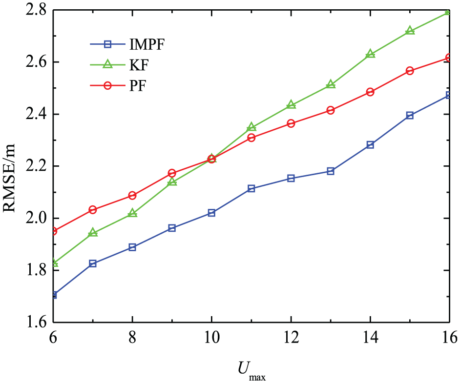
The trend of RMSE with upper limit $U_{\max }$ of uniform distribution.

NLOS error obeys the exponential distribution

In Figure 13, when ${\sigma }_i=1$ , the positioning performance of KF and PF is close, and the positioning error of IMPF is about 18% (about 0.36 m) lower than them. When ${\sigma }_i$ increases, the positioning error of the three algorithms increases, but IMPF always maintains the best positioning effect. Overall, IMPF is about 12.2% lower than PF and about 16.7% lower than KF in positioning error.

Figure 13.

The trend of RMSE with ${\sigma }_i$ under the exponential distribution.

Figure 14 shows the effect of distribution parameter when $\lambda =1$ , IMPF and KF are equivalent, and the positioning error is about 0.3 m lower than PF. However, KF is sensitive to $\lambda$ , and as $\lambda$ increases, the positioning error increases rapidly. The PF and IMPF algorithms are relatively stable. As the parameters increase, the positioning error of IMPF and PF remains at about 0.3 m, and the difference from KF increases from close to 0 to nearly 1 m. Similar to Figure 12, when $\lambda$ becomes larger, the NLOS error distribution is more uniform, so the RMSE of PF will gradually be lower than that of KF. When $\lambda =8$ , the performance of IMPF is improved by 14.0% and 24.8% when compared with PF and KF.

Figure 14.

The trend of RMSE with increasing exponential distribution parameter $\lambda$ .

Computational complexity analysis

In addition to positioning accuracy, computational complexity is also an important factor. The simulation uses runtime to express the computational complexity. The three algorithms are coded using MATLAB R2017a in the Windows 10 PC. The running time is calculated through the MATLAB $\mathrm{tic}\_\mathrm{toc}$ functions for elapsed time. The running time can reflect the complexity of the algorithm. The more complex the algorithm, the larger the calculation, and the longer the running time. As shown in Figure 15, KF obtains the lowest running time, and PF has the highest one. PF must spend some time generating and adjusting particles, and each node has its particles, causing the longest running time. In IMPF, all fixed nodes use common particles, so the computation complexity of IMPF is much lower than that of PF.

Figure 15.

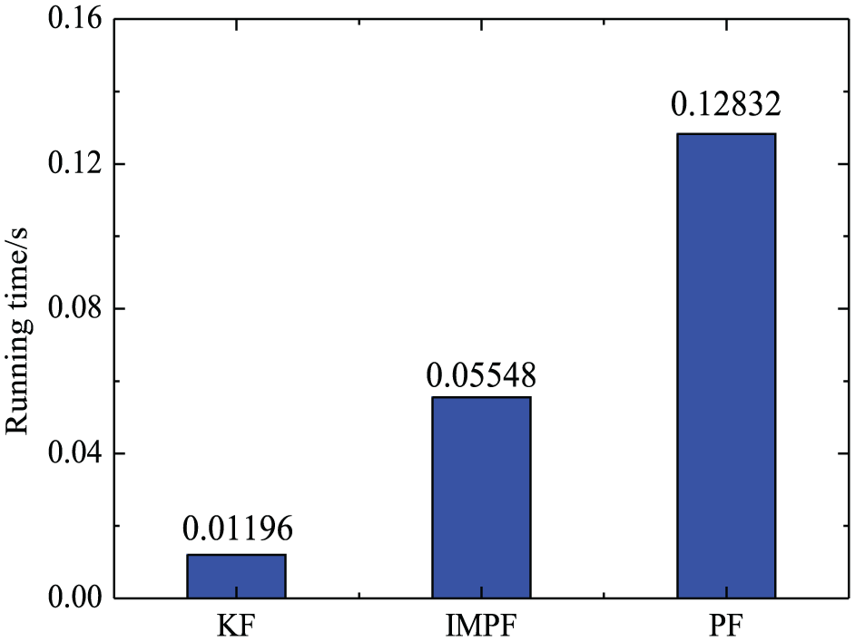
Comparison of running time in different algorithms.

Comparison with other positioning algorithms

To further demonstrate the performance of the algorithm, we simply compare it with several other algorithms—two novel positioning algorithms: sparse pseudo-input gaussian process (SPGP) ²¹ and import vector machine (IVM), ²² and an algorithm based on PF: joint particle filter (JPF). ²³ SPGP is an NLOS mitigation method based on sparse pseudo-input gaussian process, and IVM is based on import vector machine.

All of them consider the problem of NLOS. Figure 16 shows the comparison of localization error. It can be seen that the positioning error of IMPF is better than that of JPF, which is also based on particle filtering. In addition, although IMPF is slightly worse than the other two latest algorithms, the three are very close. The average positioning errors of SPGP, IVM, and IMPF are about 0.85, 1.12, and 1.25 m, respectively.

Figure 16.

Comparison of localization error with other algorithms.

We further compared the running time of IMPF, IVM, and SPGP, and the result is shown in Figure 17. IMPF runs significantly less time than the other two algorithms. Combining Figures 16 and 17, the performance of IMPF is better than other algorithms.

Figure 17.

Comparison of running time with other algorithms.

Conclusion

The article proposes an IMPF algorithm, and residual is applied to the algorithm to enhance the accuracy of the positioning results. IMPF uses residuals to weight particles and select reasonable ones. Furthermore, the proposed algorithm does not make any assumptions about the distribution of NLOS errors, which means that IMPF is robust to different types of NLOS errors. Simulation results confirm the robustness of IMPF. In addition, IMPF estimates the distance from the mobile node to the fixed node, which can also be used to estimate the coordinates of the target.

The overall work of the future is to optimize the algorithm, because the algorithm is relatively simple, and the experiment only verifies our original idea. In order to get closer to the real world, we will try to add more channel noise to the simulation. At the same time, we will consider incorporating the algorithm into other new frameworks.