Sage Journals: Discover world-class research

Abstract

To obtain the health status of long-span cable-stayed bridges, multiple sensors are applied to the health monitoring system for data collection. The optimal layout of sensors that aims to obtain as much structural information as possible with fewer sensors is important to ensure the effectiveness of the health monitoring system. Sensors are usually placed in typical locations where the structural response is obvious, and most studies utilize static response for the determination of sensor location. In fact, bridges primarily suffer the dynamic load, of which the response has a significant impact on the structural health. In this article, an optimal sensor layout method for a long-span cable-stayed bridge based on dynamic response is proposed under the consideration of vehicle–bridge coupled vibration. With vehicle load applied onto different lanes, the dynamic responses of different bridge members are obtained, and the number and the location of cable force sensors are determined according to the distribution of cable dynamic coefficient D_C, and the number and the location of displacement and strain sensors are determined according to the distribution of D_GD and D_GM, which are the dynamic load allowance for girder deflection and bending moment, respectively. The results prove that this method can reduce the number of sensors effectively and obtain bridge state information more perfectly.

Keywords

Cable-stayed bridge vehicle–bridge coupled vibration optimal layout of sensors dynamic load allowance moving load

Introduction

Bridges play an important role in the transportation system. In recent years, the span of bridges has become larger and the structural form has become more complicated. Despite the rapid development of bridge engineering, there still much sudden bridge damage occurred that threatens people’s lives seriously. Thus, an increasing number of bridges are equipped with a structural health monitoring (SHM) system. The SHM system grasps the real-time bridge health status by analyzing the collected data and provides the structural anomalies forecasting and the maintenance strategies. The SHM system obtains data through sensors, the more sensors there are, the more detailed data which contain the bridge information can be obtained. However, a large number of sensors will increase the system budget, overburden the bridge structure, and bring about data redundancy. The feasible measure to overcome the extra burden is to arrange a certain number of sensors in the most appropriate locations. Hence, optimal sensor placement (OSP) is a crucial issue of SHM.

To solve the key problem of SHM, there are plenty of research studies on OSP all over the world. For instance, Kammer¹ proposed the effective independent (EI) method based on Fisher matrix. All possible measurement points are taking into consideration, and the Fisher matrix is formed by the modal matrix of structure at first. Subsequently, the measurement points with the smallest contribution to the independence of the modal matrix are deleted in turn and the Fisher information matrix is optimized. The sensor placement is determined by minimizing the norm of Fisher matrix. Obviously, the EI method has a vast calculating amount, and sensor information loss occurs at a low-energy position. Papadopoulos and Garcia² noticed and solved such a problem by introducing driving point residue into the EI method. Heo et al.³ proposed the kinetic energy (KE) method, which is similar to the EI method except the KE matrix was maximized to obtain the sensor position. Another energy-based method named eigenvector product (EVP) method was proposed by Larson et al.;⁴ points with the maximum EVP value are selected as the location of sensors to obtain the maximum measured vibration energy. Meo and Zumpano^5,6 put forward the variance method (VM) and evaluated the effectiveness of sensor placement scheme through the signal strength and the anti-interference ability. The result proved that VM is feasible to obtain an effective arrangement scheme and the optimal sensor quantity. Chang and Pakzad⁷ further proposed the modified variance (MV) method based on principal component analysis, which determined the signal strength of each position through the covariance of the deformed matrix. On contrary to the traditional method which arranged most sensors in the middle span area of the bridge, the MV method arranged sensors nearly uniformly on the main span with low calculation cost. In addition, there are other mature methods of OSP such as Modal Assurance Criteria (MAC) method, EI-MAC hybrid method, and so on.^8,9

Traditional methods mentioned before are focused on the optimization of structural modal matrix or structural energy, and they face the dilemma of computational efficiency. Essentially, sensor placement in SHM is an optimization problem that regards the location of sensors as the variable. Hence, several studies adopted optimization algorithms to improve computational efficiency. Soman et al.¹⁰ took the genetic algorithm (GA) to obtain a multi-type sensor layout scheme for long-span bridges, which improved the overall quality of the sensor network. Shan et al.¹¹ put forward an improved GA to optimize sensor placement of a steel truss cable-stayed bridge, which replaced individual encoding with dual structure encoding and introduced adaptive probabilities of crossover and mutation to get the global optimal solution. It overcomes the shortcomings of other GAs such as slow convergence and local optimum. He et al.¹² proposed the modal strain energy (MSE)-adaptive genetic algorithm (AGA) hybrid optimization algorithm to solve the OSP problem, and MSE was used to provide the initial arrangement of sensors first to ensure the data collected by sensors have high accuracy and signal-to-noise ratio. Afterward, the AGA was introduced to determine the optimal number and location of sensors, which improved the computational efficiency greatly. In addition to GA, simulated annealing (SA) algorithm, monkey algorithm, and discrete optimization based on artificial bee colony are also used to solve the OSP problem.^13–16 Guo et al.¹⁷ proposed the information entropy–based OSP method to monitor the random ship collision damage of long-span bridges. To provide the sensor placement, a multi-objective optimization algorithm was introduced to minimize the information entropy index in each ship collision case. All the optimization algorithms above are data-driven methods. Furthermore, the OSP problem can be solved from other perspectives. Beygzadeh et al.¹⁸ put forward that the sensor position is the projection of elliptic noise on the response space plane from a geometric perspective, and the optimal position was obtained by the regularization of elliptic noise through filtering factor. Bhuiyan et al.¹⁹ proposed a sensor layout scheme with high network communication efficiency, low complexity, and strong fault tolerance from the perspective of wireless network transmission.

The purpose of OSP is to ensure the SHM system obtains structural health state effectively by analyzing data collected by sensors. Structure health state is revealed by structural vibration characteristics. Although the data-driven methods have high computational efficiency, they lack the consideration of structural vibration characteristics. Debnath et al.²⁰ proposed the modal contribution of output energy (MCOE) method based on bridge operation modes, in which the MCOE was taken as the index to evaluate the modal participation, thus determining sensor placement. Flynn and Todd²¹ developed an OSP method based on the Bayesian probability model of structural damage mode for guided wave-based SHM. Castro-Triguero et al.²² considered the parameter uncertain in wood structure and optimized the sensor position based on Fisher information matrix. Chen et al.²³ put forward the sensor optimal layout method based on a real-time modified finite element model, where construction monitoring and completion load test results were introduced to modify the finite element model of a long-span cable-stayed bridge, which was combined with the MAC method to determine the sensor position. Castro-Triguero et al.²⁴ studied the influence of parametric uncertain such as elastic modulus, mass density, and section size on the optimal placement of bridge sensors. Four classical methods were used to determine the sensor layout scheme, respectively, two based on Fisher information matrix and two based on energy matrix. It was found that bridge parameters have effects on bridge operation mode; furthermore, the signal concentrated areas are under the influence of bridge mode shape. It indicates that, for bridge SHM, the arrangement of sensors is closely related to the bridge dynamic response.

Long-span cable-stayed bridges require a large quantity of sensors for their structural information collection due to the structural complexity. Nevertheless, numerous sensors increase the structural burden and generate excessive data to confuse the extraction of structural information. To reduce the quantity of sensors, meanwhile ensure the structural stress condition is effectively reflected, the typical position of the mechanical response of cable-stayed bridge is usually selected to place sensors. The majority of current studies focus on structural static responses; in practice, a bridge is subjected to several external loads during operation, especially random vehicle loads. Vehicle–bridge coupling has a significant impact on the dynamic response of bridge; thus, the vehicle load influence on the distribution of bridge dynamic signal should be considered when determining the layout scheme of sensors. This article takes Liaohe Super-Large Bridge of Liaoning coastal highway as the research object and conducts the analysis of bridge–vehicle coupled vibration. Taking the force characteristics of different parts of a cable-stayed bridge under vehicle loads into consideration, an OSP method based on vibration mode and dynamic response for long-span cable-stayed bridges is proposed in this article.

Vehicle–bridge coupled vibration

Unlike other civil engineering structures, highway bridges are primarily subjected to the moving vehicle load during their operation. As a vehicle passes through a bridge, bridge vibration will occur under the excitation of the initial vibration of the vehicle and the unevenness of bridge deck. And conversely, the vibration of bridge structure will exert an influence on the vibration of vehicle. The mutual influence of vibration between the vehicle and the bridge is called vehicle–bridge coupled vibration.

Vibration equation of the bridge

According to the theory of structural dynamics, the dynamic equations of bridge can be written as follows

[M_{b}] {{\overset{\cdot\cdot}{U}}_{b}} + [C_{b}] {{\overset{\cdot}{U}}_{b}} + [K_{b}] {U_{b}} = {F_{b}}

(1)

in which {F_b} denotes the load vector induced by the moving vehicles and [M_b], [C_b], and [K_b] denote the mass matrix, damping matrix, and stiffness matrix, respectively. Furthermore, {U_b} is the displacement of the bridge, the first derivative of the displacement is the vibration velocity, and the second derivative of the displacement is the vibration acceleration. It is worth noting that the equation and all these symbols are described in the Cartesian coordinate system.

To reduce the degree of freedom, the modal synthesis method is adopted in this article, and the displacement of bridge structure can be expressed by the method of mode superposition

{U_{b}} = [ϕ'] {q}

(2)

in which $[ϕ']$ denotes the matrix of vibration mode composition of bridge structure and {q} denotes the coordinates of bridge structure in the regular coordinate system.

By substituting equation (2) into bridge vibration equation (1), the projection of equation (1) in regular coordinates is obtained

[M_{B}] {\overset{\cdot\cdot}{q}} + [C_{B}] {\overset{\cdot}{q}} + [K_{B}] {q} = {F_{B}}

(3)

in which [M_B], [C_B], [K_B], and [F_B] denote the mass matrix, damping matrix, stiffness matrix, and loading vector in canonical coordinates, respectively.

To facilitate the calculation, when the calculation model matrix of the bridge structure is obtained, the mass normalization should be carried out

[M_{B}] = {[ϕ]}^{T} [M_{b}] [ϕ] = [E]

(4)

in which [E] denotes unit matrix and [ϕ] denotes the vibration mode matrix treated by normalization.

Similarly, the damping matrix, stiffness matrix, and external loading vector of the bridge are shown as follows

\begin{matrix} \begin{matrix} [C_{B}] = [\begin{matrix} 2 ξ_{1} ω_{1} & \dots & 0 \\ ⋮ & ⋱ & ⋮ \\ 0 & \dots & 2 ξ_{n} ω_{n} \end{matrix}] \\ [K_{B}] = [\begin{matrix} ω_{1}^{2} & \dots & 0 \\ ⋮ & ⋱ & ⋮ \\ 0 & \dots & ω_{n}^{2} \end{matrix}] \\ [F_{B}] = {[ϕ]}^{T} {F_{b}} \end{matrix} \end{matrix}

in which ξ_n denotes the damping ratio of the ith mode and ω_n denotes vibration frequency of the ith mode.

Vibration equation of the vehicle

In this article, the vehicle with multi-axles is adopted and the spatial model is established. Several assumptions are made about the vehicle model. The wheel and the bridge will contact with each other tightly all the time. Only vertical effects between the vehicle and the bridge are considered, while longitudinal and transverse effects are ignored. The vehicle body and all wheels are assumed as rigid with corresponding masses, while the spring and the damper are linear. The vehicle model can be seen in Figure 1.

Figure 1.

Vehicle model.

According to the theory of structural dynamics, the dynamic equations of vehicle can be written as

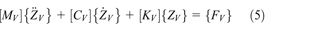
[M_{V}] {{\overset{\cdot\cdot}{Z}}_{V}} + [C_{V}] {{\overset{\cdot}{Z}}_{V}} + [K_{V}] {Z_{V}} = {F_{V}}

(5)

in which {F_V} denotes the load vector induced by the bridge and [M_V], [C_V], and [K_V] denote the mass matrix, damping matrix, and stiffness matrix of the vehicle, respectively. Furthermore, {Z_V} is the displacement of the vehicle, the first derivative of the displacement is the vibration velocity, and the second derivative of the displacement is the vibration acceleration.

The mass matrix, displacement vector, and load vector of the vehicle model are, respectively, shown as follows

[M_{V}] = diag {m_{s}, J_{y}, J_{x}, m_{t 1}, m_{t 2}, m_{t 3}, \dots, m_{t 2 n}}

(6)

in which m_s denotes the mass of the vehicle body, m_ti denotes the mass of the ith vehicle wheel, and J_y and J_x denote, respectively, the moment of inertia of longitudinal swing and transversal swing

{U_{V}} = col {U_{s}, θ_{s}, α_{s}, U_{t 1}, U_{t 2}, \dots, U_{t 2 n}}

(7)

in which U_s denotes the vertical vibration degree of the vehicle body, U_ti denotes the vertical vibration degree of the ith vehicle wheel, and θ_s and α_s denote, respectively, the vibration degree of longitudinal swing and transversal swing

{F_{V}} = col {0, 0, 0, k_{t 1} Δ_{1} + c_{t 1} {\overset{\cdot}{Δ}}_{1}, k_{t 2} Δ_{2} + c_{t 2} {\overset{\cdot}{Δ}}_{2}, \dots \infty, k_{t 2 n} Δ_{2 n} + c_{t 2 n} {\overset{\cdot}{Δ}}_{2 n}}

(8)

in which Δ_i denotes the relative displacement of the contact point between wheel and bridge deck and k_ti and c_ti denote, respectively, the stiffness coefficient and damping coefficient of the ith vehicle wheel.

The damping matrix of the vehicle model is divided into four parts by taking the boundary line between the vehicle body and the wheel

[C_{V}] = [\begin{matrix} C_{V 11} & C_{V 12} \\ C_{V 21} & C_{V 22} \end{matrix}]

(9)

\begin{array}{l} [C_{V 11}] = [\begin{matrix} \sum_{i = 1}^{n} c_{s 2 i - 1} + c_{s 2 i} & - \sum_{i = 1}^{n} a_{i} (c_{s 2 i - 1} + c_{s 2 i}) & - \sum_{i = 1}^{n} (b_{1} c_{s 2 i - 1} + b_{2} c_{s 2 i}) \\ - \sum_{i = 1}^{n} a_{i} (c_{s 2 i - 1} + c_{s 2 i}) & \sum_{i = 1}^{n} a_{i}^{2} (c_{s 2 i - 1} + c_{s 2 i}) & - \sum_{i = 1}^{n} (b_{1} a_{i} c_{s 2 i - 1} + b_{2} a_{i} c_{s 2 i}) \\ - \sum_{i = 1}^{n} (b_{1} c_{s 2 i - 1} + b_{2} c_{s 2 i}) & - \sum_{i = 1}^{n} (b_{1} a_{i} c_{s 2 i - 1} + b_{2} a_{i} c_{s 2 i}) & \sum_{i = 1}^{n} (b_{1}^{2} c_{s 2 i - 1} + b_{2}^{2} c_{s 2 i}) \end{matrix}] \\ [C_{V 12}] = [\begin{matrix} - c_{s 1} & - c_{s 2} & \dots & - c_{s 2 n} \\ a_{1} c_{s 1} & a_{1} c_{s 2} & \dots & a_{n} c_{s 2 n} \\ - b_{1} c_{s 1} & - b_{2} c_{s 2} & \dots & - b_{2} c_{s 2 n} \end{matrix}] \\ [C_{V 21}] = [\begin{matrix} - c_{s 1} & a_{1} c_{s 1} & - b_{1} c_{s 1} \\ - c_{s 2} & a_{1} c_{s 2} & - b_{2} c_{s 2} \\ ⋮ & ⋮ & ⋮ \\ - c_{s 2 n} & a_{n} c_{s 2 n} & - b_{1} c_{s 2 n} \end{matrix}] \end{array}

in which k_si and c_si denote, respectively, the stiffness coefficient and damping coefficient of the suspension system of the ith vehicle wheel.

Similarly, when calculating the stiffness matrix of the vehicle model, C and c in the damping matrix are changed to K and k, respectively, which will not be discussed here.

Vibration equation of the vehicle–bridge coupled system

In the vehicle–bridge coupled vibration system, the force of the wheel induced by bridge vibration is

F_{t i} = - k_{t i} Δ_{i} - c_{t i} {\overset{\cdot}{Δ}}_{i}

(10)

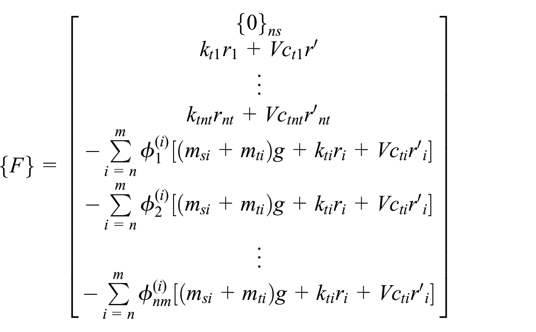
According to the vibration equation of the bridge model and vehicle model established above, the corresponding equation of vehicle–bridge coupled vibration system can be obtained

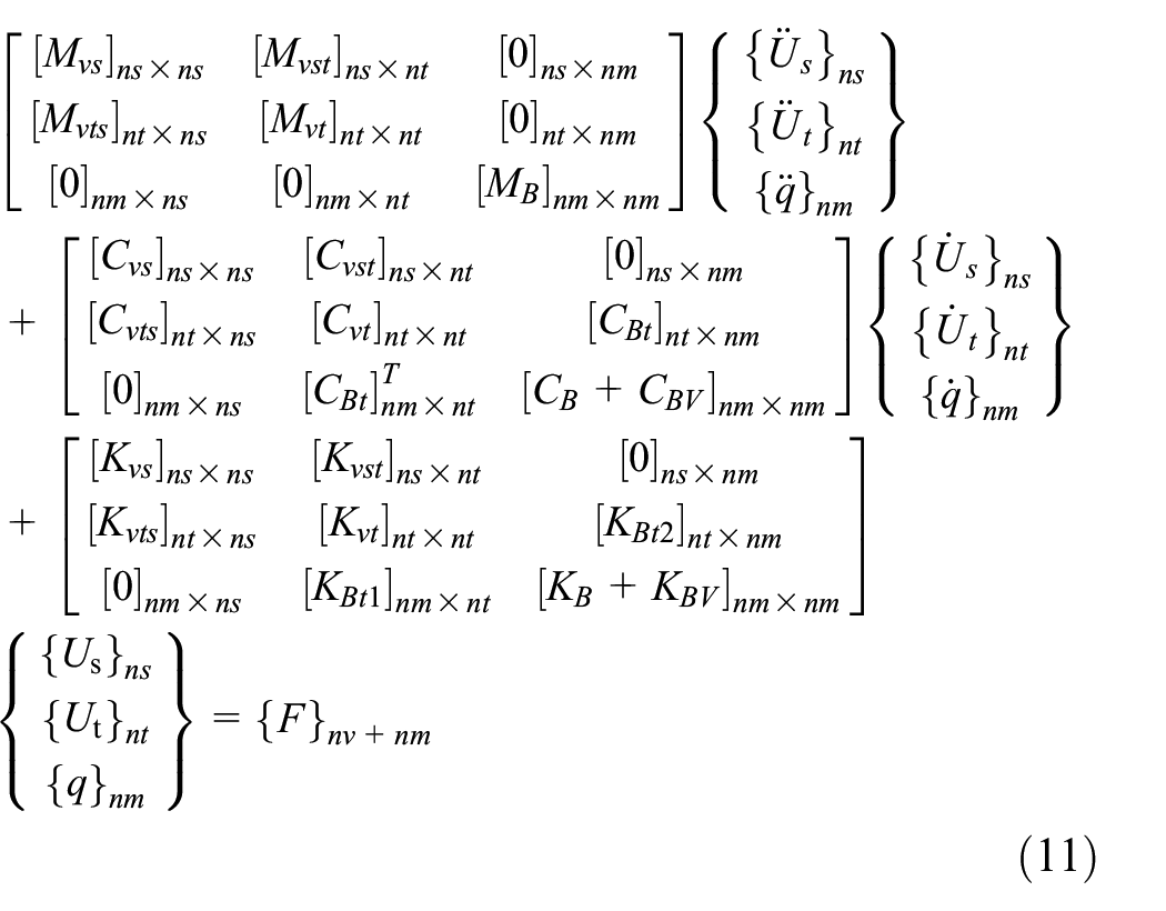
\begin{matrix} [\begin{matrix} {[M_{vs}]}_{ns \times ns} & {[M_{vst}]}_{ns \times nt} & {[0]}_{ns \times nm} \\ {[M_{vts}]}_{nt \times ns} & {[M_{vt}]}_{nt \times nt} & {[0]}_{nt \times nm} \\ {[0]}_{nm \times ns} & {[0]}_{nm \times nt} & {[M_{B}]}_{nm \times nm} \end{matrix}] {\begin{matrix} {{\overset{\cdot\cdot}{U}}_{s}}_{ns} \\ {{\overset{\cdot\cdot}{U}}_{t}}_{nt} \\ {\overset{\cdot\cdot}{q}}_{nm} \end{matrix}} \\ + [\begin{matrix} {[C_{vs}]}_{ns \times ns} & {[C_{vst}]}_{ns \times nt} & {[0]}_{ns \times nm} \\ {[C_{vts}]}_{nt \times ns} & {[C_{vt}]}_{nt \times nt} & {[C_{Bt}]}_{nt \times nm} \\ {[0]}_{nm \times ns} & {[C_{Bt}]}_{nm \times nt}^{T} & {[C_{B} + C_{BV}]}_{nm \times nm} \end{matrix}] {\begin{matrix} {{\overset{\cdot}{U}}_{s}}_{ns} \\ {{\overset{\cdot}{U}}_{t}}_{nt} \\ {\overset{\cdot}{q}}_{nm} \end{matrix}} \\ + [\begin{matrix} {[K_{vs}]}_{ns \times ns} & {[K_{vst}]}_{ns \times nt} & {[0]}_{ns \times nm} \\ {[K_{vts}]}_{nt \times ns} & {[K_{vt}]}_{nt \times nt} & {[K_{Bt 2}]}_{nt \times nm} \\ {[0]}_{nm \times ns} & {[K_{Bt 1}]}_{nm \times nt} & {[K_{B} + K_{BV}]}_{nm \times nm} \end{matrix}] \\ {\begin{matrix} {U_{s}}_{ns} \\ {U_{t}}_{nt} \\ {q}_{nm} \end{matrix}} = {F}_{nv + nm} \end{matrix}

(11)

in which nm denotes the number of vibration modes of bridge, nv denotes the degree number of all vehicles, ns denotes the degree number of vehicle body, and nt denotes the degree number of vehicle wheels

[C_{Bt}] = [\begin{matrix} ϕ_{1}^{(1)} c_{t 1} & ϕ_{2}^{(1)} c_{t 1} & \dots & ϕ_{nm}^{(1)} c_{t 1} \\ ϕ_{1}^{(2)} c_{t 2} & ϕ_{2}^{(2)} c_{t 2} & \dots & ϕ_{nm}^{(2)} c_{t 2} \\ ⋮ & ⋮ & ⋱ & ⋮ \\ ϕ_{1}^{(nt)} c_{tnt} & ϕ_{2}^{(nt)} c_{tnt} & \dots & ϕ_{nm}^{(nt)} c_{tnt} \end{matrix}]

[C_{B} + C_{BV}] = [\begin{matrix} C_{1} + \sum_{i = n}^{m} ϕ_{1}^{(i)} c_{ti} ϕ_{1}^{(i)} & \sum_{i = n}^{m} ϕ_{1}^{(i)} c_{ti} ϕ_{2}^{(i)} & \dots & \sum_{i = n}^{m} ϕ_{1}^{(i)} c_{ti} ϕ_{nm}^{(i)} \\ \sum_{i = n}^{m} ϕ_{2}^{(i)} c_{ti} ϕ_{1}^{(i)} & C_{2} + \sum_{i = n}^{m} ϕ_{2}^{(i)} c_{ti} ϕ_{2}^{(i)} & \dots & \sum_{i = n}^{m} ϕ_{2}^{(i)} c_{ti} ϕ_{nm}^{(i)} \\ ⋮ & ⋮ & ⋱ & ⋮ \\ \sum_{i = n}^{m} ϕ_{nm}^{(i)} c_{ti} ϕ_{1}^{(i)} & \sum_{i = n}^{m} ϕ_{nm}^{(i)} c_{ti} ϕ_{2}^{(i)} & \dots & C_{nm} + \sum_{i = n}^{m} ϕ_{nm}^{(i)} c_{ti} ϕ_{nm}^{(i)} \end{matrix}]

[K_{Bt 1}] = - [\begin{matrix} k_{t 1} ϕ_{1}^{(1)} & k_{t 2} ϕ_{1}^{(2)} & \dots & k_{tnt} ϕ_{1}^{(nt)} \\ k_{t 1} ϕ_{2}^{(1)} & k_{t 2} ϕ_{2}^{(2)} & \dots & k_{tnt} ϕ_{2}^{(nt)} \\ ⋮ & ⋮ & ⋱ & ⋮ \\ k_{t 1} ϕ_{nm}^{(1)} & k_{t 2} ϕ_{nm}^{(2)} & \dots & k_{tnt} ϕ_{nm}^{(nt)} \end{matrix}]

\begin{matrix} [K_{Bt 2}] = {[K_{Bt 1}]}^{T} - V [\begin{matrix} c_{t 1} ϕ_{1}'^{(1)} & c_{t 1} ϕ_{2}'^{(1)} & \dots & c_{t 1} ϕ_{nm}'^{(1)} \\ c_{t 2} ϕ_{1}'^{(2)} & c_{t 2} ϕ_{2}'^{(2)} & \dots & c_{t 2} ϕ_{nm}'^{(2)} \\ ⋮ & ⋮ & ⋱ & ⋮ \\ c_{tnt} ϕ_{1}'^{(nt)} & c_{tnt} ϕ_{2}'^{(1)} & \dots & c_{tnt} ϕ'_{nm}^{(nt)} \end{matrix}] \\ = - [\begin{matrix} k_{t 1} ϕ_{1}^{(1)} + V c_{t 1} ϕ_{1}'^{(1)} & k_{t 2} ϕ_{1}^{(2)} + V c_{t 1} ϕ_{2}'^{(1)} & \dots & k_{tnt} ϕ_{1}^{(nt)} + V c_{t 1} ϕ_{nm}'^{(1)} \\ k_{t 1} ϕ_{2}^{(1)} + V c_{t 2} ϕ_{1}'^{(2)} & k_{t 2} ϕ_{2}^{(2)} + V c_{t 2} ϕ_{2}'^{(2)} & \dots & k_{tnt} ϕ_{2}^{(nt)} + V c_{t 2} ϕ_{nm}'^{(2)} \\ ⋮ & ⋮ & ⋱ & ⋮ \\ k_{t 1} ϕ_{nm}^{(1)} + V c_{tnt} ϕ_{1}'^{(nt)} & k_{t 2} ϕ_{nm}^{(2)} + V c_{tnt} ϕ_{2}'^{(1)} & \dots & k_{tnt} ϕ_{nm}^{(nt)} + V c_{tnt} ϕ'_{nm}^{(nt)} \end{matrix}] \end{matrix}

[K_{B} + K_{BV}] = [\begin{matrix} K_{1} + \sum_{i = n}^{m} ϕ_{1}^{(i)} (k_{ti} ϕ_{1}^{(i)} + V c_{ti} ϕ_{1}'^{(i)}) & \dots & \sum_{i = n}^{m} ϕ_{1}^{(i)} (k_{ti} ϕ_{nm}^{(i)} + V c_{ti} ϕ'_{nm}^{(i)}) \\ ⋮ & ⋱ & ⋮ \\ \sum_{i = n}^{m} ϕ_{nm}^{(i)} (k_{ti} ϕ_{1}^{(i)} + V c_{ti} ϕ_{1}'^{(i)}) & \dots & K_{nm} + \sum_{i = n}^{m} ϕ_{nm}^{(i)} (k_{ti} ϕ_{nm}^{(i)} + V c_{ti} ϕ'_{nm}^{(i)}) \end{matrix}]

{F} = [\begin{matrix} {0}_{ns} \\ k_{t 1} r_{1} + V c_{t 1} r' \\ ⋮ \\ k_{tnt} r_{nt} + V c_{tnt} {r'}_{nt} \\ - \sum_{i = n}^{m} ϕ_{1}^{(i)} [(m_{si} + m_{ti}) g + k_{ti} r_{i} + V c_{ti} {r'}_{i}] \\ - \sum_{i = n}^{m} ϕ_{2}^{(i)} [(m_{si} + m_{ti}) g + k_{ti} r_{i} + V c_{ti} {r'}_{i}] \\ ⋮ \\ - \sum_{i = n}^{m} ϕ_{nm}^{(i)} [(m_{si} + m_{ti}) g + k_{ti} r_{i} + V c_{ti} {r'}_{i}] \end{matrix}]

To solve the complicated problem of vehicle–bridge coupled vibration, the program Vehicle-Bridge Coupled Vibration Analysis (VBCVA) has been completed by our own research group.²⁵

Description and dynamic characteristics of the bridge

Description of the bridge

Liaohe Super-Large Bridge is a cable-stayed bridge with double pylons and double cable planes which is located in Liaoning coastal highway. The layout of the bridge span is 62.3 + 152.7 + 436 + 152.7 + 62.3 m, which can be seen in Figure 2.

Figure 2.

The layout of the bridge (cm).

The lateral layout of the bridge is 0.15 (guardrail) + 1.45 (cable anchorage zone) + 0.4 (anti-collision guardrail) + 2.5 (non-motorized lane) + 11.25 (motorized lane) + 1.5 (intermediate zone) + 11.25 (motorized lane) + 2.5 (non-motorized lane) + 0.4 (anti-collision guardrail) + 1.45 (cable anchorage zone) + 0.15 (guardrail) = 33 m, which can be seen in Figure 3.

Figure 3.

Typical cross-section of the main girder (cm).

Longitudinal movable supports are installed at the junction of auxiliary piers, transition piers, and towers, while transverse limit devices and longitudinal dampers are installed at the junction of towers and beams. As a result, the bridge is a semi-floating system.

The main girder is a streamlined flat steel box girder. The height of the girder inner contour at the centerline is 3 m, the full width of the girder which including two end air nozzles is 33 m, and the width of per air nozzle is 1.4 m. The two-way transverse slope is set on the bridge deck, while the slope is 2%. The roof of the steel box girder is 20 and 16 mm in thickness. The floor thickness is 12 mm in the mid-span section (D), while it is 14 mm in the tower-girder joint section (A, B, C) and the bracket assembly section (H, I, J, G). The U-shaped stiffening ribs are set on the roof and floor in the whole length range of the main girder. The thickness of the U-shaped stiffening ribs is 10 mm which are corresponding to the 20-mm-thick roof and the thickness of other U-shaped stiffening ribs corresponding to the rest of the roof is 8 mm, while the thickness of the U-shaped stiffening ribs corresponding to the floor is 6 mm. There are four longitudinal webs in the steel box girder. The thickness of the side webs is 30 mm. The middle webs can be solid webs, mixed webs, and truss webs; the truss webs are composed of welded T-bars.

The stayed cables are sectoral-arranged, and the transverse distance of anchorage points is 30.94 m, while the standard distance of stay cables on the main beam is 15.0 m. The first pair of cables to the intersection of tower and beam is 17.7 m away from the pylon. A galvanized parallel wire cable system with double high-density polyethylene (HDPE) sheath is adopted. The specifications of the cables are 223 filaments, 4 filaments, 199 filaments, 3 filaments, 163 filaments, 3 filaments of 139 filaments, and 1 filament of 163 filaments in the order of A14-A1 and H14-H1, respectively. The longest cable is 237.662 m and the shortest is 72.935 m.

The depth of epoxy asphalt concrete pavement is 5 cm. The bonding layer is built between the epoxy asphalt concrete and the bridge deck. C50 concrete is applied to the pylon column, cross-beam, transition pier, and auxiliary pier of main bridge, while Q345qE is adopted in the steel box girder plate.

Dynamic characteristics of the bridge

The finite element model of the bridge is established by ANSYS. BEAM4 is used to simulate the main girder, piers, and towers, while LINK180 is used to simulate cables. To simulate different lanes, the spatial grillage model is adopted for the main girder, which is shown in Figure 4. The finite element model of the whole bridge is presented in Figure 5.

Figure 4.

Spatial grillage model of the main girder.

Figure 5.

Finite element model of the bridge.

Combined with the structural characteristics of the steel box girder and the convenience of vehicle loading, the lane is divided into 11 longitudinal beams, of which both sides and the centerline are virtual longitudinal beams, while the other longitudinal beams corresponding to the location of the lane, respectively. According to the theory of the grillage method, the neutral axis of each longitudinal beam cross-section is translated to ensure that it is in the same position as the original neutral axis of the overall section. The rigidity and weight of the longitudinal beam are selected according to the actual value, while the beam is only considered with its rigidity contribution but ignored with the weight because the weight has been considered in the calculation of the longitudinal beam.

Vibration modes are inherent and integral characteristics of elastic structures, including modes, frequencies, and damping, of which damping is usually obtained by actual measurement. The modal results of the bridge obtained by software ANSYS are illustrated in Figure 6.

Figure 6.

Modal results of the bridge: (a) First-order symmetric mode (f₁ = 0.360 Hz), (b) First-order antisymmetric mode (f₂ = 0.489 Hz), (c) Second-order symmetric mode (f₃ = 0.793 Hz), and (d) Second-order antisymmetric mode (f₄ = 0.893 Hz).

Obviously, the low-order modes play a major role in the dynamic response of bridge structures. To acquire the basic characteristics of each mode more accurately, the elevation maps of the first four vertical bending modes are summarized in Figure 7.

Figure 7.

Summary of modal results.

According to Figure 7, the peak positions of each order modes can be observed clearly. In other words, the maximum response can be obtained when sensors are placed in these positions, which is more conducive to the acquisition of bridge structural modes. The position of characteristic points of each mode is summarized in Table 1. Among them, L₁, L₂, and L₃ are the lengths of side span, secondary side span, and middle span, respectively.

Table 1.

Feature points of mode shapes.

Mode shape	X-coordinate of feature points	Be expressed as the span length
1st symmetric	39.8 129.8 433.0	0.64L₁ 0.44L₂ 0.50L₃
1st antisymmetric	39.8 129.8 352.7	0.64L₁ 0.44L₂ 0.32L₃
2nd symmetric	39.8 129.8 300.2 433.0	0.64L₁ 0.44L₂ 0.20L₃ 0.50L₃
2nd antisymmetric	39.8 129.8 247.7 367.7	0.64L₁ 0.44L₂ 0.08L₃ 0.35L₃

Combining Figure 7 and Table 1, it is obvious that the first-order symmetric and antisymmetric vertical bending modes have three characteristic points, while the second-order symmetric and antisymmetric vertical bending modes have four characteristic points. If the first four vertical bending modes need to be acquired effectively, a total of seven locations need to be arranged after removing some repetitive measuring points. Furthermore, considering that the measuring point 0.32L₃ is close to 0.35L₃, the average value 0.34L₃ would be adopted. As a result, six locations for sensors need to be arranged when taking the vibration mode of bridge structure into consideration. They are 0.64L₁, 0.44L₂, 0.08L₃, 0.20L₃, 0.34L₃, and 0.50L₃.

It should be noted that the characteristic positions of side span and secondary span are not in their middle position. For common cable-stayed bridges, the middle span is the longest, the secondary span is the second in length, and the side span is the shortest, which means that the stiffness of the middle span, the secondary span, and the side span increases in turn. Therefore, the characteristic position of the secondary is in the direction of the side span, while the sensitive position of the side span is far from the position of the side fulcrum.

Optimal layout of sensors based on dynamic response of the bridge

Numerical simulation

A three-axle truck with a total weight of 35 tons is selected. The specific parameters are given in Gao.²⁶ The dynamic responses of cables and main girder are analyzed when the vehicle passes through the bridge at a constant speed along different lanes. The vehicle speed is 5, 10, 15, 20, 25, 30, 35, and 40 m/s. Meanwhile, lane 2, lane 3, lane 4, and centerline in Figure 4 are selected, respectively. It should be noted that lane 1 is neglected as it is a non-motorized lane. To obtain some of the stress essences easier, vehicle is assumed to travel along the centerline on the symmetrical structure in this article, despite the fact that the centerline is not a lane.

For the convenience of expression, half of the bridge structure and the unilateral cables are taken into account and numbered as shown in Figure 8.

Figure 8.

Number of cables.

When a moving vehicle passes through a bridge, the dynamic response of the bridge excited by the vehicle vibration is more intense than that under the static vehicle load. For cables, the change of their axial force should be paid more attention. The dynamic coefficient D_C is introduced as follows

D_{C} = \frac{F_{dynamic}}{F_{stat}} - 1

(12)

where D_C is the dynamic coefficient of the cable, F_dynamic is the axial force of the cable due to moving vehicles, and F_stat is the axial force of the cable due to static vehicular loads.

Dynamic responses of cables subjected to moving vehicles along different lanes are shown in Figure 9.

Figure 9.

Dynamic responses of cables: (a) the moving vehicle in lane 2, (b) the moving vehicle in lane 3, (c) the moving vehicle in lane 4, and (d) the moving vehicle in the centerline.

According to Figure 9, the dynamic response of stay cables has a positive correlation with increases in the speed no matter which lane the vehicle is in. The dynamic coefficients of stay cables are the smallest when the vehicle runs in lane 2 but the largest when the vehicle runs in lane 3.

It should be noted that when the vehicle is in lane 2, the dynamic coefficients of the two cables near the pylon are larger, the dynamic coefficients of the long cables near the fulcrum are smaller, and the dynamic coefficients of the other cables are basically the same. When the vehicle is in lane 3, the dynamic coefficients of the long cables and the short cables are smaller, while the dynamic coefficients of the middle length cables are larger. When the vehicle is in lane 4, the short cables near the pylon are not obvious, and the dynamic coefficients of other cables are basically the same.

In conclusion, the regularity of the dynamic coefficient for the short cables near the pylon is not obvious, the long cables near the fulcrum can be properly concerned, and the middle cables have little differences. Hence, we can focus on the short cables near the pylon and the long cables near the fulcrum to design the sensor layout scheme; meanwhile, one middle cable should be chosen representatively. Specifically speaking, the cable force sensors for the bridge could be arranged by cables A14, A9, A2, A1, H1, H2, and H14. It can effectively avoid the defect of the traditional method which requires the arrangement of a large number of cable force sensors.

Dynamic responses of the girder

The variety of girder displacement and moment demands more attention; thus, the dynamic load allowance D_GD and D_GM are introduced

D_{GD} = \frac{y_{dynamic}}{y_{stat}} - 1

(13)

where D_GD is the dynamic load allowance for vertical displacement of the girder, y_dynamic is the vertical displacement of the girder due to moving vehicles, and y_stat is the vertical displacement of the girder due to static vehicular loads

D_{GM} = \frac{M_{dynamic}}{M_{stat}} - 1

(14)

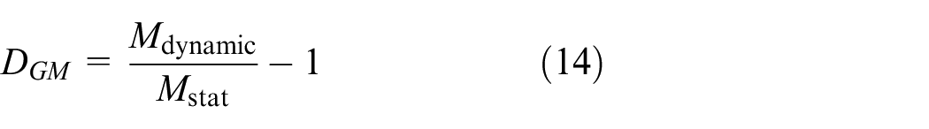
where D_GM is the dynamic load allowance for positive moment of the girder, M_dynamic is the positive moment of the girder due to moving vehicles, and M_stat is the positive moment of the girder due to static vehicular loads.

Dynamic responses of the girder subjected to moving vehicles along different lanes are shown in Figures 10 and 11.

Figure 10.

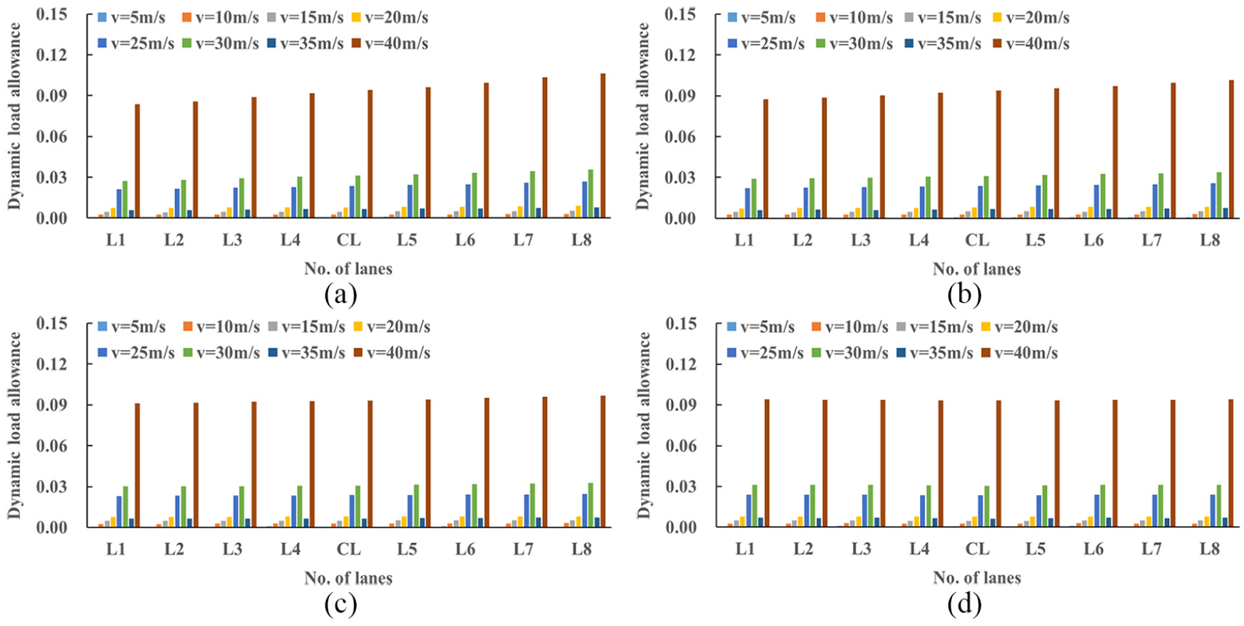
Dynamic load allowance (displacement) of the girder: (a) the moving vehicle in lane 2, (b) the moving vehicle in lane 3, (c) the moving vehicle in lane 4, and (d) the moving vehicle in the centerline.

Figure 11.

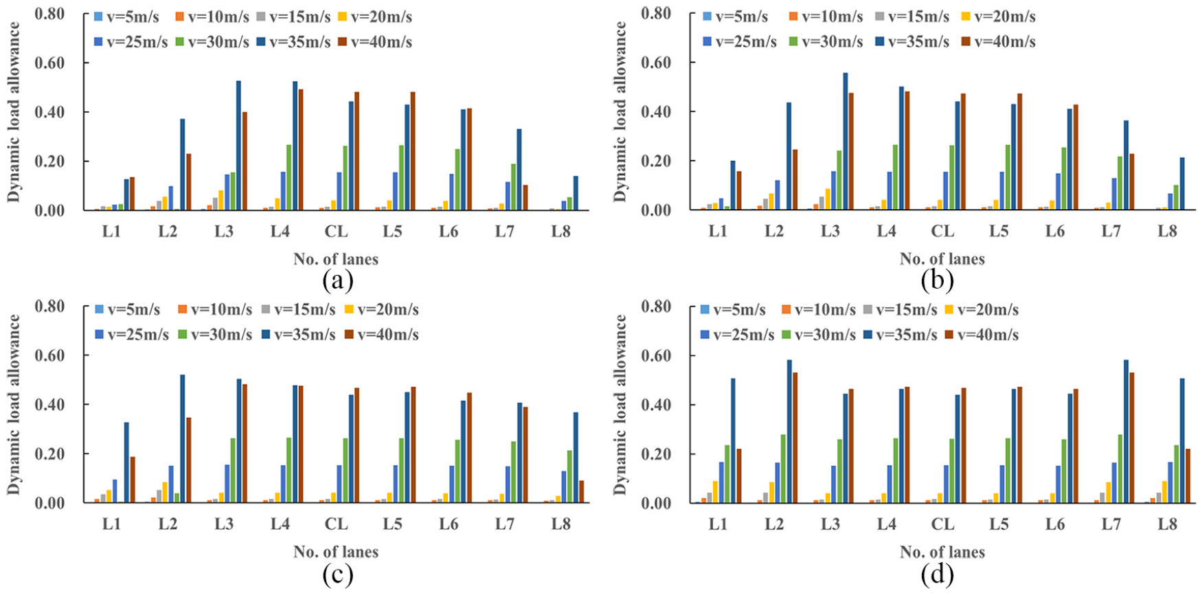
Dynamic load allowance (moment) of the girder: (a) the moving vehicle in lane 2, (b) the moving vehicle in lane 3, (c) the moving vehicle in lane 4, and (d) the moving vehicle in the centerline.

It is illustrated in Figure 10 that the dynamic load allowance of the main girder does not increase monotonously with the change of velocity for the vertical displacement in the middle span. When the vehicle is located in different lanes, the dynamic load allowance corresponding to different transverse positions of the main girder is consistent with the change of speed; in other words, they fluctuate upward. The driving speed of trucks is generally less than 80 km/h. The calculation results in this article show that when the speed is less than 20 m/s, the dynamic load allowance presents a monotonous upward trend.

It is worth noticing that lane 8 which is away from lane 2 has the largest dynamic load allowance when the vehicle is in lane 2. The reason is that the vibration amplitude of the main girder corresponding to different lanes is basically the same when moving vehicle loads across the bridge. Although the corresponding dynamic amplification factor is larger, the overall effect is still small as the static response of the lane corresponding to the driving position far from the vehicle becomes smaller. In addition, the closer the vehicle is to the centerline, the more uniform the dynamic load allowance of the main girder corresponding to each lane is. Moreover, the dynamic load allowance changes linearly along the transverse direction due to the large stiffness of the main girder.

Therefore, only two vertical displacement sensors need to be arranged for the girder.

As can be seen from Figure 11, the dynamic load allowance of the main girder does not increase monotonously with the change in speed for the mid-span moment. When the vehicle is in different lanes, the dynamic load allowance corresponding to different transverse positions of the main girder varies with the speed. When trucks run within their normal speed range, which is less than 20 m/s, the dynamic load allowance increases monotonously.

Therefore, as for the layout of strain sensors about the main girder, each lane should be arranged at the bottom of the girder. Correspondingly, there are eight strain sensors.

Conclusion

Considering that the bridge structure is mainly subjected to dynamic loads, an optimal layout of sensors for long-span cable-stayed bridges based on vehicle–bridge coupling vibration analysis is proposed in this article. The finite element model of the whole bridge is established, in which the main girder is simulated by spatial grillage model and the lanes were divided. A three-axle truck with a total weight of 35 tons is taken as the vehicle load, which is loaded on different lanes at different speeds to obtain the dynamic responses of cables and main girders.

The first few modes of cable-stayed bridge dominate the dynamic response. To obtain effective structural information, sensors can be arranged at the peak points of the main modes. For the Liaohe bridge in this article, taking the first two symmetric and antisymmetric modes into consideration, sensors are placed at positions 0.64L₁, 0.44L₂, 0.08L₃, 0.20L₃, 0.34L₃, and 0.50L₃, respectively.

When vehicles are loaded in different lanes, D_C of short cables near the bridge tower has no significant changing rules, while that of long cables near the fulcrum change obviously. Thus, the layout of cable force sensors requires much attention on the symmetrical long cables and short cables. In addition, as D_C of middle cables has little differences, it is adequate to choose one middle cable as representative. In this article, the cable force sensors are arranged by A14 (long cable), A9 (middle cable), A2, A1 (short cables), H1, H2, and H14.

When vehicles are loaded in different lanes, D_GD of each transverse position of the main beam presents linear change from one side to the other side. The closer the loading position is to the beam centerline, the more uniform the distribution of D_GD in each transverse position is. Therefore, only two displacement sensors of main beam should be arranged in the beam bottom of the mid-span section.

When vehicles are loaded in different lanes, the distribution of D_GD in each transverse position of main beam is different. The strain sensors of main beam should be placed at beam bottom corresponding to each lane. The bridge in this article has eight lanes, and eight strain sensors are placed correspondingly.

The proposed method can effectively reduce the number of sensors, and the collected data can effectively reflect the dynamic state of bridges. The conclusions of this article can be used as the reference for sensor optimal layout of similar long-span cable-stayed bridges.

Footnotes

Handling Editor: Xiangyang Xu

Declaration of conflicting interests

The author(s) declared no potential conflicts of interest with respect to the research, authorship, and/or publication of this article.

Funding

The author(s) disclosed receipt of the following financial support for the research, authorship, and/or publication of this article: This research was financially supported by the National Natural Science Foundation of China (Grant No. 51778194), the China Postdoctoral Science Foundation (Grant No. 2017M621282), the Fundamental Research Funds for the Central Universities (Grant No. HIT. NSRIF. 2019056), the Transportation Science and Technology Plan Project of Jilin Province (Grant No. 2015-1-14), and the Key Subject of Education Science in Heilongjiang Province (Grant No. GZB1319026).

ORCID iD

Qingfei Gao

References

Kammer

. Sensor placement for on-orbit modal identification and correlation of large space structures. J Guid Control Dynam 1991; 14(2): 251–259.

Papadopoulos

Garcia

. Sensor placement methodologies for dynamic testing. AIAA J 1998; 36(2): 256–263.

Heo

Wang

Satpathi

. Optimal transducer placement for health monitoring of long span bridge. Soil Dyn Earthq Eng 1997; 16(7–8): 495–502.

Larson

Zimmerman

Marek

. A comparison of modal test planning techniques: excitation and sensor placement using the NASA 8-bay truss. P Soc Photo: Opt Ins 1994; 2251: 205–211.

Meo

Zumpano

. Optimal sensor placement on a large-scale civil structure. P Soc Photo: Opt Ins 2004; 5394: 108–117.

Meo

Zumpano

. On the optimal sensor placement techniques for a bridge structure. Eng Struct 2005; 27(10): 1488–1497.

Chang

Pakzad

. Optimal sensor placement for modal identification of bridge systems considering number of sensing nodes. J Bridge Eng 2014; 19(6): 04014019.

Carne

Dohrmann

. A modal test design strategy for model correlation. In: Proceedings of the 13th international modal analysis conference, vol. 2460, Nashville, TN, 13–16 February 1995, pp.927–933. Bethel, CT: Society for Experimental Mechanics.

Aimin

. Optimal sensor placement of cable-stayed bridge using mixed algorithm based on effective independence and modal assurance criterion methods. J Vib Meas Diagn 2009; 29(1): 55–59.

10.

Soman

Onoufriou

Votsis

, et al. Optimization of multi-type sensor placement for SHM based on application demands. IABSE Symp Rep 2013; 101(1): 1–9.

11.

Shan

Wan

Qiao

. Optimal sensor placement for long-span railway steel truss cable-stayed bridge. In: 2011 third international conference on measuring technology & mechatronics automation, Shangshai, China, 6–7 January 2011. New York: IEEE.

12.

Xing

, et al. A combined optimal sensor placement strategy for the structural health monitoring of bridge structures. Int J Distrib Sens N 2013(5–6): 1–9.

13.

, et al. Sensor placement optimization in structural health monitoring using niching monkey algorithm. Int J Struct Stab Dy 2014; 14(5): 1440012.

14.

Zhang

. A modified monkey algorithm for optimal sensor placement in structural health monitoring. Smart Mater Struct 2012; 21(10): 105033.

15.

a G

Huang

, et al. Optimal placement of sensors in monitoring for bridge based on hybrid genetic algorithm. J Vib Eng 2008; 21(2): 191–196.

16.

Sun

Bueyuekoeztuerk

. Optimal sensor placement in structural health monitoring using discrete optimization. Smart Mater Struct 2015; 24(12): 125034.

17.

Guo

Chen

. Optimal sensor placement for damage detection of bridges subject to ship collision. Struct Control Health Monit 2017; 24: e1963.

18.

Beygzadeh

Salajegheh

Torkzadeh

, et al. Optimal sensor placement for damage detection based on a new geometrical viewpoint. Mol Cell Biol 2013; 27(13): 47–54.

19.

Bhuiyan

MZA

Wang

Cao

. Sensor placement with multiple objectives for structural health monitoring in WSNs. In: IEEE international conference on embedded software and systems (ICESS2012), Liverpool, 25–27 June 2012, pp.699–706. New York: IEEE.

20.

Debnath

Dutta

Deb

. Placement of sensors in operational modal analysis for truss bridges. Mech Syst Signal Pr 2012; 31: 196–216.

21.

Flynn

Todd

. Bayesian probabilistic structural modeling for optimal sensor placement in ultrasonic guided wave-based structural health monitoring. P Soc Photo: Opt Ins 2010; 7648: 76480Z.

22.

Castro-Triguero

Saavedra Flores

Diazdelao

, et al. Optimal sensor placement in timber structures by means of a multi-scale approach with material uncertainty. Struct Control Health Monit 2014; 21(12): 1437–1452.

23.

Chen

Zhou

Shen

. Sensor placement of long-term health monitoring for large bridges based on the real-time correction of finite element model. J Chongqing Univ 2013; 12(3): 123–130.

24.

Castro-Triguero

Murugan

Friswell

, et al. Optimal sensor placement for structures under parametric uncertainty. In: International modal analysis conference, Garden Grove, CA, 11–14 February 2013. New York: Springer.

25.

Gao

Wang

, et al. Dynamic load allowance in different positions of the multi-span girder bridge with variable cross-section. J Vibroeng 2015; 17(4): 2025–2039.

26.

Gao

. Design and evaluation methods on dynamic performance of girder bridges under moving vehicle loads. PhD Thesis, Harbin Institute of Technology, Harbin, China, 2015.

Optimal layout of sensors in large-span cable-stayed bridges subjected to moving vehicular loads

Abstract

Keywords

Introduction

Vehicle–bridge coupled vibration

Vibration equation of the bridge

Vibration equation of the vehicle

Vibration equation of the vehicle–bridge coupled system

Description and dynamic characteristics of the bridge

Description of the bridge

Dynamic characteristics of the bridge

Optimal layout of sensors based on dynamic response of the bridge

Numerical simulation

Dynamic responses of the girder

Conclusion

Footnotes

Declaration of conflicting interests

Funding

ORCID iD

References