A deep learning platooning-based video information-sharing Internet of Things framework for autonomous driving systems

Abstract

To enhance the safety and stability of autonomous vehicles, we present a deep learning platooning-based video information-sharing Internet of Things framework in this study. The proposed Internet of Things framework incorporates concepts and mechanisms from several domains of computer science, such as computer vision, artificial intelligence, sensor technology, and communication technology. The information captured by camera, such as road edges, traffic lights, and zebra lines, is highlighted using computer vision. The semantics of highlighted information is recognized by artificial intelligence. Sensors provide information on the direction and distance of obstacles, as well as their speed and moving direction. The communication technology is applied to share the information among the vehicles. Since vehicles have high probability to encounter accidents in congested locations, the proposed system enables vehicles to perform self-positioning with other vehicles in a certain range to reinforce their safety and stability. The empirical evaluation shows the viability and efficacy of the proposed system in such situations. Moreover, the collision time is decreased considerably compared with that when using traditional systems.

Introduction

Autonomous control technologies gradually entered the vehicle market, including adaptive cruise control (acceleration/deceleration), automated emergency braking, and lane-changing and lane-keeping system for locking onto a path, resulting in full autonomy of a self-driving car. The sensory perception system is composed of many subsystems responsible for tasks such as car localization, static obstacles mapping, moving objects detection and tracking, road mapping, and traffic signalization detection and recognition, among others.

As a matter of fact, autonomous driving began in the 1980s when Navlab vehicles, which functioned in structured environments, were presented by Carnegie Mellon University (Pittsburgh, PA). ¹ Subsequently, the University of the Bundeswehr Munich (UniBw Munich, Neubiberg, Germany) reported early results of high-speed motorway driving. ² In the Eureka PROMETHEUS project in 1994, UniBw Munich and Daimler-Benz showed that autonomous driving reached a speed of 130 km/h in three-lane French Autoroute traffic, which included tracking other vehicles and lane markings. The system determined when the vehicle would change between lanes by itself, although a human driver was required to approve the decisions for safety reasons. ³

Autonomous or self-driving vehicles are typically trained offline before they are allowed to perform in the real world.^4,5 However large the training dataset might be, in real-world driving, a vehicle is bound to come across unexpected situations (e.g., accident) where it needs to act (steer, brake, etc.) quickly. Moreover, the detecting instrument without penetration function cannot detect objects that are occluded by other vehicles. Consequently, blind areas where objects cannot be detected remain. This limitation causes autonomous vehicles to be incapable of handling emergency situations. If future information can be obtained by current vehicle from a reliable source, such as from another vehicle traversing the same road in front of the current vehicle or a drone or satellite, it will get more time to act. This “future” data presented to the vehicle is a salient data point as it would have been unexpected given the model learned by the vehicle. The question “how can this data point be used by the vehicle to safely mitigate the unexpected situation?” is the main objective of this work.

If platooning-based information-sharing technology is used in autonomous driving, then vehicles can share the situations among themselves. The obstacles occluded by A can also be detected by B through the approach in which A sends the positions of obstacles that are relative to A and its own position. We can then calculate the positions of obstacles that are relative to B.

In this study, a camera, radar, and lidar instrument are used to detect obstacles rather than just relying on high-definition mapping and localization techniques. Furthermore, convolutional neural networks (CNNs) are applied to realize classification and recognition. The proposed system enables vehicles to commute and share detected information and perform self-positioning with one another in a platoon by wireless devices. We select the WiMAX (Worldwide Interoperability for Microwave Access) technique as a wireless communication method due to its long transmission distance and high transmission rate. After receiving information from other vehicles in a platoon, a vehicle constructs the circumstance of surrounding obstacles by analyzing information and becomes capable of abating blind areas. Finally, the dynamic window approach (DWA) algorithm is adopted to plan the path, proportional–integral–derivative (PID), and model predictive control (MPC) that are applied in vehicle control.

The rest of this article is organized as follows: Section “Related work” presents work related to this study. The proposed approach is detailed in section “Methodology.” Experiments are described and discussed in section “Experimental evaluation,” and conclusions are drawn in section “Conclusion and future directions.”

Related work

In 2012, lane detection was used to facilitate lane departure warnings ⁶ for drivers and reinforce the driver heading control in lane-keeping assist systems. The detection and tracking of vehicles driving ahead was utilized in adaptive cruise control systems ⁷ to keep a safe and comfortable distance. Precrash systems, which trigger full braking power to reduce damage if a driver reacted slowly, also emerged. ⁸

In 2014, Mercedes-Benz ⁹ successfully exhibited a demonstration on a Class S 500 that was equipped with close-to-production sensor hardware and solely relied on vision and radar sensors combined with accurate digital maps to gain a comprehensive understanding of complex traffic circumstances.

In 2016, a 4WIS4WID^10,11 vehicle was proposed, in which the judgments of vision with the fuzzy control methods were integrated to ensure the correct motion of the vehicle. The vehicle was able to change its velocity in a timely manner under any condition and was able to move in a curved and narrow lane successfully. Two inner loops ⁹ of simultaneous localization and mapping helped improve perception and planning performances. An algorithm was presented by adding an inner loop to the perception system to expand the detection range of sensors. The other inner loop obtained practical feedback to restrain mutations of two adjacent planning periods.

Google’s automatic vehicle project Waymo ¹² has been shown to distinguish the obstruction between pedestrians and cars. It calculates their velocity and predicts their motion paths the very next moment. Waymo’s software determines the trajectory, speed, lane, and steering maneuvers needed to progress along the route safely. Despite significant contributions in autonomous driving, the project still needs more testing to get fully matured.

With the development of integrated and miniaturization techniques, additional instruments installed on vehicles outside have been much smaller than those installed on earlier autonomous vehicles.

Methodology

Installation of cameras and sensors

The methodology of installation of cameras and sensors is adoptive from the architecture of Baidu’s Apollo autonomous vehicle. Figure 1(a) shows the structure of Baidu’s Apollo, which uses multisensor fusion to improve perception performance and is a basic example of modern autonomous vehicles, whereas Figure 1(b) shows an image of a real autonomous vehicle with almost the same sensor installed. This vehicle was used in DARPA Urban Challenge 2007.

Figure 1.

The autonomous vehicles and the major sensors: (a) a structure of Baidu’s Apollo autonomous vehicle ¹³ and (b) an autonomous vehicle with sensors installed: cameras, lidars, and GPS antennas. ⁸

Lidar sensors are used to detect obstacles in the distance. These sensors are usually installed on the top to acquire optimum vision. The detection result is classified via point cloud segment, and then the type, distance, and velocity of the obstacles are determined.

Cameras mainly have three tasks to perform. The first is to recognize objects, which is different from lidar that recognizes objects via CNNs. The second is to recognize traffic lights. With the classification of red and green lights and GPS location on map, vehicles can decide to go straight or turn left/right or wait for traffic lights. The third task is to track lanes, as shown in Figure 2. This feature is necessary for vehicles in order to drive on modern streets.

Figure 2.

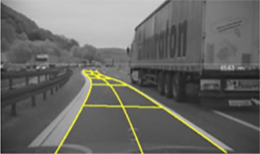
Lane tracking on a marked highway. ⁸

Radar sensors mainly detect nearby objects. These sensors are usually installed around vehicles at the margin to ensure that the vehicles do not contact other objects accurately.

GPS is used with the help of a high-resolution map to determine the location of vehicles at the centimeter level. A wireless device is also installed to accomplish information sharing. We calculate the relative positions of objects that are occluded by other vehicles connected.

Vehicles detect surrounding obstacles using camera, lidar, radar, GPS, and inertial sensors that are commonly available in the market. Four cameras, a 32-layer lidar, a 4-layer lidar, a millimeter-wave radar, and a GPS+ inertial sensor are utilized. ¹⁴ The distribution method is similar to that of Google’s autonomous driving framework, and the statistics are shown in Figure 3. The main advantage of this distribution is that it can cover most of the areas surrounding the vehicle and adapt to various traffic situations and weather conditions. However, the expenditure of this distribution is high, and it is not very suitable for parking tasks because distances less than 1 m are undetectable.

Figure 3.

The detection distribution statistics of sensors for an autonomous vehicle.

Classification, tracking, and segmentation using CNNs

CNN, as the most important algorithm used in advanced driver-assistance systems and automotive automatic vision systems, is expected to play an important role in fully automatic driving. CNN is efficient in analyzing scenes. This algorithm divides scenes into recognizable objects until objects, pedestrians, cars, trucks, shoulders, and landmarks in the scenes can be recognized in the camera system.^15–17 CNNs can learn how to recognize and extract information from the scenes when driving in real time by using a large amount of training data. For example, corners/bends can be found through various layers of CNN, and the next objects are loops, road signs, and the meaning of road signs. This information is transmitted to the sensor and fused with data from other sensors, such as lidar or radar. Flash warnings or controlling brakes or steering through a multimedia interactive system can be issued to understand the situation and respond to the scenes.

CNNs include multiple categories of layers in which all information is fed through. These layers are stacked in a hierarchical pattern and consist of convolutional layers, pooling layers, fully connected (FC) layers, and a loss layer. Each type of layer has its own concentration and objective in the procedure of analyzing data. With each consecutive layer, the analysis turns to more abstract form. In the field of image recognition, this indicates that the first layers react to stimuli such as light intensity changes or oriented fields, whereas the later layers decide the identification of objects and make intelligent evaluation on its importance. This behaves as a large generalization of the pattern layers to “search for” in an image. These layers are based on the mathematical functions contained by their neurons to process pixels of the image. While all layers are composited by neurons, not all of them serve for the same objective.

Figure 4 shows a typical CNN structure beginning with convolutional layers with increasing complexity and ending in an FC layer to extract the data. With the help of the FC layer arranged at the end, the network can collect in-depth data in varied dimensions through its convolutional layers and extract these data to a readable output included in the final FC layer. ¹⁸ We select VGG16-Places365 as the basic model for location recognition because it shows the best performance on multiple datasets. Beginning with LeNet-5, ¹⁹ CNNs usually have standard stacked convolution layers (optionally, followed by batch normalization and maximum pooling), followed by one or more FC layers. VGG16-Places335 has the same structure as that of VGG (Visual Geometry Group), which consists of 16 weight layers, including 13 convolution layers and 3 FC layers. The Places dataset contains more than 10 million images with 365 unique scene categories; therefore, the size of the last FC layer should be modified to 365. The 13 convolution layers are divided into five parts, each with the same data dimension. Behind each part, a maximum aggregation layer exists, which is executed through a 2 × 2 pixel window with a span of 2. Following the stack of convolution layers are three FC layers: the first two layers have 4096 channels, and the third layer performs 365 channel location classifications, thereby comprising 365 channels (one for each category). In addition to these layers, the last layer is the soft-max layer, and all hidden layers are equipped with rectifier linear unit nonlinearity.

Figure 4.

Example of the typical layered structure of a CNN. ¹⁸

CNNs can learn advanced semantic features at various levels of abstraction through deep architecture. However, spatial information of images is lost through FC layers, which may not be ideal in applications such as visual location recognition. The experimental results in Chen et al. ²⁰ and Bai et al. ²¹ show that the deep features based on CNN generated in the convolution layer perform better than those of the FC layer in loop closure detection. We modify the CNN model by adding several pool layers and deleting the FC layers to reduce feature size and save image-processing time. After adjusting the features of the three layers to one dimension, we use the connection operation ²² to fuse them.

Visual features are among the most important factors that affect the accuracy of image matching. Our method uses the CNN features extracted from the given CNN model rather than the traditional handmade features to calculate the similarity among images. Floating point is the type of CNN functionality that we ultimately acquire from the module. We name this feature F_cnn, which has a dimension of 1 × 100,352. A practical way to reduce the cost of image matching is to convert feature vectors into binary codes, which can be used for fast comparison with the Hamming distance. We first standardize each element into 8-bit integers and then obtain the integer characteristics $F_{\mathrm{cnn}}^{\mathrm{std}}$ , as shown in equation (1). They can be easily converted into binary features $F_{\mathrm{cnn}}^{\mathrm{bin}}$

$$F_{\mathrm{cnn}}^{\mathrm{std}}=\frac{F_{\mathrm{cnn}}-\min \left(F_{\mathrm{cnn}}\right)}{\max \left(F_{\mathrm{cnn}}\right)-\min \left(F_{\mathrm{cnn}}\right)}\times 255$$

(1)

The use of a binary descriptor to match the Hamming distance is fast and effective and is adopted to calculate the distance among images. We have determined in many studies that the similarity of two frames can be calculated by matching a single image, and therefore, we can calculate their Hamming distance HmmDistance _ij to represent similarity. The calculation process is

$$\begin{array}{c}\multicolumn{1}{c}{\mathrm{HmmDistanc}{\mathrm{e}}_{\mathrm{ij}}=\mathrm{HmmDistanc}{\mathrm{e}}_{\mathrm{ji}}}\\ \multicolumn{1}{c}{=\mathrm{bitsum}(F_{\mathrm{cnn}\left(i\right)}^{\mathrm{bin}}\oplus F_{\mathrm{cnn}\left(j\right)}^{\mathrm{bin}})}\end{array}$$

(2)

where $F_{\mathrm{cnn}(i)}^{\mathrm{bin}}$ and $F_{\mathrm{cnn}(j)}^{\mathrm{bin}}$ are the feature descriptors of two images. Location is considered an image sequence rather than a single image because it performs better in long-term and large-scale environments, as described in works such as Thorpe et al. ¹ and Zong et al. ⁹ In our method, we define S_length as matching the image sequence length of the current frame. Therefore, the image sequence of the first frame consists of continuous images in the range (i − S_length + 1, i), and we connect $F_{\mathrm{cnn}(i-k+1)}^{\mathrm{bin}},F_{\mathrm{cnn}(i-k+2)}^{\mathrm{bin}},\dots ,F_{\mathrm{cnn}(i)}^{\mathrm{bin}}$ to the final feature for matching. In this case, we can use the sequence information of equation (3) to obtain the distance among images. The distance is the similarity score of different places, and we keep it in the similarity matrix (M). If we find that the distance between two frames is less than the given threshold, then these positions will be successfully identified^23–25

$$\mathrm{Distanc}{\mathrm{e}}_{\mathrm{ij}}=\mathrm{Distanc}{\mathrm{e}}_{\mathrm{ji}}=\frac{\sum _{k=0}^{S_{\mathrm{length}}-1}\mathrm{HmmDistanc}{e}_{i-k,j-k}}{S_{\mathrm{length}}}$$

(3)

WiMAX data transportation

WiMAX features

IEEE 802.16 is a set of telecommunications technology standards to provide wireless access over long distances in various ways that cover point-to-point links to full-mobile cellular-type access. The WiMAX technology is a broadband wireless access technology for wireless metropolitan area networks. ²⁶ This technology supports not only fixed terminals but also portable and mobile terminals.

• 1. High transmission rate

The access speed of WiMAX can reach 70 Mbit/s. ²⁶ High transmission rate can help vehicles to exchange enough information that can be used to depict circumstances around them.

• 2. Long transmission distance

The transmission distance can be longer than 50 km theoretically. WiMAX can effectively resist attenuation and multipath effects and select different encoding technologies according to channel state and transmission rate to improve coverage and capacity. The support of spatial multiplexing, multiuser detection, self-adaptive power control, and other technologies enables WiMAX to have large coverage and capacity.

• 3. Standardization and compatibility

Reconciling standards and interoperability compatibility can be promoted on the basis of unified technical standards. Standardization and compatibility are the guarantee of popularization of technique.

Sharing GPS data in a vehicle platoon

Vehicles can detect blind areas near themselves considerably by sharing detection information in the vehicle platoon, as depicted in Figure 5. Moreover, vehicles can obtain road condition information at further distance by combining GPS and detection information; for example, car A receives information that a traffic accident occurs in the direction of 30° south to east of car B at $\mathrm{N}36°18\prime 51.743″$ , $\mathrm{E}28°05\prime 154″$ .

Figure 5.

Platooning-based information sharing among autonomous vehicles.

Calculation of the position of the occluded vehicles

By using the sharing detection information in a platoon, we can calculate the relative position from another relative position.

As shown in Figure 6, we are driving in vehicle A and obtain the angle α and distance (S_AB) to car B through detection. At this moment, object C cannot be detected by A but can be detected by B; thus, angle β and distance S_BC can be transmitted to A.

Figure 6.

Illustration of vehicles’ operation to calculate the position of invisible vehicles.

We calculate the relative position of C to A through the information sent to A by B. According to the Pythagorean theorem

$$\begin{array}{c}\multicolumn{1}{c}{S_{\mathrm{AC}}=\sqrt{{(S_{\mathrm{AB}}\sin \alpha +S_{\mathrm{BC}}\sin \beta )}^2+{(S_{\mathrm{AB}}\cos \alpha +S_{\mathrm{BC}}\cos \beta )}^2}}\\ \multicolumn{1}{c}{=\sqrt{S_{\mathrm{AB}}^2+S_{\mathrm{BC}}^2+2S_{\mathrm{AB}}{S}_{\mathrm{BC}}\cos (\alpha -\beta )}}\end{array}$$

(4)

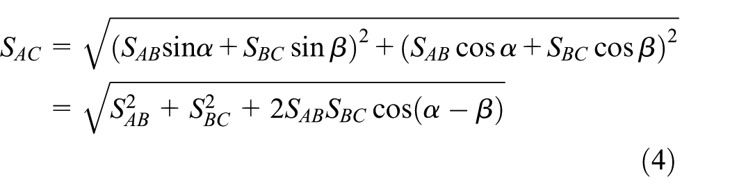
where S_AB, S_BC, and S_AC are the distances between A and B, B and C, and A and C, respectively; α is the angle between moving direction of A and vector $\overrightarrow{\mathrm{AB}}$ ; and β is the angle between moving direction of B and vector $\overrightarrow{\mathrm{BC}}$ .

According to cosine theorem

$$\theta =\alpha +\mathrm{co}{s}^{-1}\left(\frac{S_{\mathrm{AB}}^2+S_{\mathrm{AC}}^2-S_{\mathrm{BC}}^2}{2S_{\mathrm{AB}}{S}_{\mathrm{AC}}}\right)$$

(5)

where θ is the angle between moving direction of A and vector $\overrightarrow{\mathrm{AC}}$ . The magnitude of velocity can be calculated in a very short time interval, ΔT (Figure 7(a)). The length B moving in this short time duration is

$$\mathrm{\Delta }S=\mathrm{\Delta }\theta \times \frac{L+L\prime }{2}$$

(6)

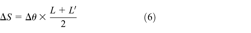
where Δθ is the change of the angle between the connecting line and perpendicular direction of moving. Then, the magnitude of velocity of B (V_BA) related to A is

$$\left|V_{BA}\right|=\frac{\mathrm{\Delta }S}{\mathrm{\Delta }T}=\frac{\mathrm{\Delta }\theta \frac{L+L^{\prime }}{2}}{\mathrm{\Delta }T}=\frac{\mathrm{\Delta }\theta \left(L+L^{\prime }\right)}{2\mathrm{\Delta }T}=\frac{\left(\theta -{\theta }^{\prime }\right)\left(L+L^{\prime }\right)}{2\mathrm{\Delta }T}$$

(7)

where ΔT is the time duration. The velocity of C (V_CB) related to B can be calculated in the same way.

Figure 7.

Calculation of the velocities V_CB and V_BA: (a) magnitude of velocity and (b) direction of velocity.

In a very short time interval, the direction can be approximately same as segment m, that is

$$m=\sqrt{L^2+{L\prime }^2-2\mathrm{LL}\prime \cos \mathrm{\Delta }\theta }$$

(8)

where α is the angle of driving direction between A and B, which is expressed as

$$\alpha =\mathrm{co}{s}^{-1}\left(\frac{L^2+m^2-{L\prime }^2}{2\mathrm{Lm}}\right)-(\frac{\pi }{2}-\theta )$$

(9)

Figure 7 illustrates the process of calculation of the magnitude and the direction of the velocities V_CB and V_CA. The velocity of C (V_CB) has been transmitted to A simultaneously, and the velocity of B (V_BA) related to A is detected by A. We then calculate the velocity of C related to A using a relative velocity formula. Here, we did not take into account the theory of relativity because a vehicle’s velocity is much lower than the velocity of light, that is

$$V_{\mathrm{CA}}=V_{\mathrm{CB}}+V_{\mathrm{BA}}$$

(10)

where V_CA is the velocity of C related to A, V_CB is the velocity of C related to B, and V_BA is the velocity of B related to A.

Once vehicle A obtains the relative position (S_AC, θ) and velocity (V_CA) of C, it can then speculate on the motion of C since A cannot detect C directly.

Planning realization using the DWA algorithm

The DWA algorithm can be divided into two parts: search space and optimization. The two parts can be further divided into three steps.

Search space

The search space of the possible velocities can be achieved in three steps:

1. Circular trajectories: Circular trajectories (curvatures) are uniquely determined by pairs (v,w) of translational and rotational velocities and are the main factors considered by the DWA. In this step, the output is two-dimensional (2D) velocity search space.

2. Admissible velocities: Only safe trajectories are considered because of the restriction to admissible velocities. If the vehicle can stop before it reaches the closest obstacle on the corresponding curvature, then A pair (v,w) is considered admissible.

3. Dynamic window: The admissible velocities are limited to those that can be reached within a short time interval given the restricted accelerations of the vehicles by the dynamic window.

Optimization

The objective of optimization maximizes the following function

$$\begin{array}{c}\multicolumn{1}{c}{G(v,w)=\sigma (\alpha ·\mathrm{heading}(v,w)+\beta ·\mathrm{dist}(v,w)}\\ \multicolumn{1}{c}{+\gamma ·\mathrm{vel}(v,w))}\end{array}$$

(11)

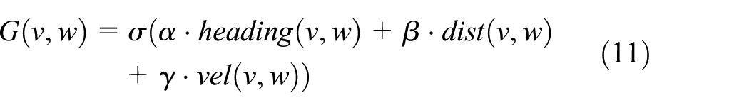
This function trades off the following three aspects in accordance with the current position and orientation of vehicles:

1. Target heading: Heading is a measure of progress toward the destination. This aspect is maximal if the vehicle moves directly toward its target.

2. Clearance: This aspect indicates the distance from the vehicle to the closest obstacle on the trajectory. The smaller the distance to an obstacle, the higher is the vehicle’s desire to move around it.

3. Velocity: vel represents the forward velocity of the vehicle.

The function σ smoothes the weighted sum of the three aspects and leads to considerable side clearance from obstacles.^27,28

Fuzzy adaptive PID and MPC

Fuzzy adaptive PID

The fuzzy adaptive PID control is devised on the basis of PID control. Its general form can be expressed as

$$u\left(t\right)=k_{p}e\left(t\right)+k_i\underset{0}{\overset{t}{\int }}e\left(t\right)\mathrm{dt}+k_d\frac{\mathrm{de}\left(t\right)}{\mathrm{dt}}$$

(12)

where k_p is the proportion coefficient, k_i is the integral coefficient, and k_d is the differential coefficient. Summation and difference quotients are usually replaced with integral and differential coefficients, respectively, in the actual control. The discretization equation can be expressed as

$$u\left(k\right)=k_{p}e\left(k\right)+k_i\sum _{i=0}^{k-1}e\left(i\right)+k_d[e\left(k\right)-e(k-1)]$$

(13)

The 2D fuzzy inference controller has two inputs and three outputs as shown in Figure 8. The inputs of the fuzzy inference controller are the deviation e and deviation change rate e_c between the expected and actual front wheel angle. The outputs are the deviation in the proportional, integral, and differential coefficients, which can be expressed as Δk_p, Δk_i, and Δk_d, respectively.

Figure 8.

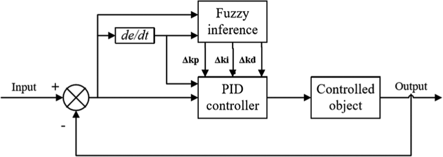
Structure of fuzzy adaptive PID controller. ²⁵

In the steering process, the deviation and deviation change rate test the fuzzy inference controller constantly. The fuzzy controller can adjust the three parameters of k_p, k_d, and k_i to meet the various requirements of e and e_c, which are deviation and deviation change rate. The vehicle can have an appropriate response and enhance the steering stability.^29–31

MPC

MPC is an advanced process control method that is used to realize process control under certain constraints. Its implementation depends on the dynamic model of the process (usually linear model). In the control time domain (for a limited period of time), it mainly optimizes the current time, considers the future time to obtain the optimal control solution of the current time, and optimizes repeatedly to achieve the optimal solution of the entire time domain.^32,33

MPC is a time-dependent method that uses the current state of the system and the current control quantity to realize the control of the future state of the system. The future state of the system is uncertain; thus, the future control quantity should be adjusted continuously according to the system state in the control process. Compared with classical PID control, MPC has the capabilities of optimization and prediction. MPC is an optimization control problem that aims to decompose a long time span, even an infinite time span, into several shorter or finite time spans for optimal control problems and still pursues the optimal solution to a certain extent.

Three steps are performed in MPC:

1. Predictive modeling is the basis of MPC, which is used to predict the future output of the system.

2. Rolling optimization, an online optimization, is used to optimize control inputs in a short time to minimize the gap between the predictive model output and reference value.

3. Feedback correction, which is based on the actual output of the controlled object at the new sampling time, corrects the output of the predictive model and then optimizes it to prevent the large gap between the control output and expectation caused by model mismatch or external interference. ³³

Experimental evaluation

Here, we provide an experimental evaluation of the proposed Internet of Things (IoT) framework.

Experimental setup

We implemented the experiments by the simulation software and achieved significant results. However, it is advised that the results should only be used as a reference. In order to simulate driving at residential districts, urban roads, and highways, we considered 20, 40, 60, and 80 km/h speed wherever appropriate:

1. We release three to five autonomous vehicles by disabling the status of platooning-based information-sharing function on a simulating road at 20, 40, 60, and 80 km/h speed. We then make dynamic obstacles move along different directions. The obstacles must satisfy the inclusion of visible and invisible objects. After the vehicles have traveled 5000 km, we count the occurrences of collisions and record them as a1, a2, a3, and a4.

2. We release three to five autonomous vehicles by enabling the platooning-based information-sharing function on a simulating road at 20, 40, 60, and 80 km/h speed. We then make dynamic obstacles move along different directions. The obstacles must satisfy the inclusion of visible and invisible objects. After the vehicles have traveled 5000 km, we count the occurrences of collisions and record them as A1, A2, A3, and A4.

3. We release only one autonomous vehicle with detectors that are completely covered on a simulating road at 20, 40, 60, and 80 km/h speed. We then make dynamic obstacles move along different directions. The obstacles must satisfy the inclusion of visible and invisible objects. After the vehicle has traveled 5000 km, we count the occurrences of collisions and record them as b1, b2, b3, and b4.

4. We release three to five autonomous vehicles that turn on platooning-based information-sharing function on a simulating road at 20, 40, 60, and 80 km/h speed. We completely cover the detectors of one of the vehicles. We then make dynamic obstacles move along different directions. The obstacles must satisfy the inclusion of visible and invisible objects. After the vehicles have traveled 5000 km, we count the collision that occurs on the vehicle with completely covered detectors and record them as B1, B2, B3, and B4. After performing several experiments, we record the average results and report them in the following section.

Results and discussion

Figure 9 shows the result statistics for all test groups with respect to speed and collision times. For Test 1, we switched off the wireless device in the proposed platooning-based information-sharing framework and obtained the collision times of 21.4, 35.8, 51.2, and 84.4 against the speeds of 20, 40, 60, and 80 km/h, respectively. This scenario and performance is almost the same as that available in most common autonomous vehicles today. As we have predicted, collisions increase as velocity increases. The reaction distance decreases as velocity increases. When invisible and moving obstacles emerge suddenly, inevitable collisions usually happen.

Figure 9.

Collision times in four different tests at various simulation speeds.

In contrast to Test 1, Test 2 is conducted by switching on the wireless device. After they are connected with each other, autonomous driving becomes safe and predictable. An obvious decrease in collision times occurs, especially when vehicles are moving at high speeds. The problem caused by reaction distance is insufficient due to the platooning-based information-sharing function because vehicles obtain information on invisible moving obstacles.

Test 3 shows the worst results, which indicate that if the detectors do not function, then the vehicle would lose all safety. We set this test mainly to simulate the most possible dangerous case that autonomous vehicles may meet, namely, sensors are invalid. We switch off the wireless device to perform a contrast experiment. Numerous collisions occur. In this case, autonomous vehicles cannot guarantee the security of passengers.

We then switch on the wireless device to conduct Test 4. Collision times are still high but have improved. Vehicles can obtain information indirectly through other vehicles connected to them. In sum, the four tests prove that platooning-based information sharing has a positive effect on autonomous vehicles.

Conclusion and future directions

We improved the performance of autonomous vehicles by adding a platooning-based information-sharing function to decrease the risk of crashing when detectors are covered and invisible moving obstacles suddenly appear. In other words, when the platooning-based information-sharing mode is enabled, the autonomous vehicles can notice and predict the obstacles in advance. The vehicles can plan and avoid the obstacles accurately and enhance the safety in contrast to vehicles without platooning-based information-sharing mode or that do not switch on this functionality.

In the future, we aim to optimize the path standing on a higher level, that is, by designing an algorithm that enables vehicles to move cooperatively to save fuel and time. We also intend to separate the different status of vehicles and utilize them to improve accuracy and security. For instance, separating high-speed vehicles from low-speed vehicles can save time and enhance safety. Such improvements should be considered after the safety of autonomous vehicles is sufficiently high and stable. At any time, the safety of autonomous vehicles is always the most important consideration. In addition, with the application of 5G in the future, there will be a potential to reduce the latency of information transmission significantly.^34,35