
Abstract
Vision-based techniques are widely used in micro aerial vehicle autonomous landing systems. Existing vision-based autonomous landing schemes tend to detect specific landing landmarks by identifying their straightforward visual features such as shapes and colors. Though efficient to compute, these schemes only apply to landmarks with limited variability and require strict environmental conditions such as consistent lighting. To overcome these limitations, we propose an end-to-end landmark detection system based on a deep convolutional neural network, which not only easily scales up to a larger number of various landmarks but also exhibit robustness to different lighting conditions. Furthermore, we propose a separative implementation strategy which conducts convolutional neural network training and detection on different hardware platforms separately, i.e. a graphics processing unit work station and a micro aerial vehicle on-board system, subject to their specific implementation requirements. To evaluate the performance of our framework, we test it on synthesized scenarios and real-world videos captured by a quadrotor on-board camera. Experimental results validate that the proposed vision-based autonomous landing system is robust to landmark variability in different backgrounds and lighting situations.
Introduction
In recent years, Unmanned Aerial Vehicles (UAVs) have been widely utilized in both military and civilian fields, such as military real-time monitoring, resource exploration, civil surveillance, cargo transportation and agricultural planning. 1 One key issue for safely applying UAVs to these tasks is to maneuver UAV flights in an accurate manner. Traditional UAV flights tend to be controlled through human manipulation with certain navigational aids. State-of-the-art UAV flights operate in an autonomous manner, which not only unleashes human labor but also enables safer and more accurate maneuvers. Specifically, three basic phases for UAV autonomous flights include takeoff, hovering and landing. 2 Among them, autonomous landing is the most crucial phase because 80% of the UAV accidents occur during landing. 3 Therefore, how to build robust autonomous landing systems has become one of the most important and challenging topics for the UAV research. 4
Existing autonomous landing systems of UAVs can be roughly classified into two groups, i.e. electromagnetically guided landing systems and vision-based landing systems. The electromagnetically guided landing systems include those based on inertial navigation systems (INS) and global positioning systems (GPS). INS provides instant positioning information but cannot guarantee long-term positioning accuracy. GPS provides a global availability in open areas but may incur positioning errors up to 10 m and may be blocked by buildings. 5 The electromagnetic landing systems are suitable for large scale landing problems (e.g. a large sized UAV landing on a large open area) with considerable tolerance for position errors. However, they cannot be straightforwardly applied to micro aerial vehicle (MAV) landing problems, which require accurate positioning within a small sized space. The electro-optical navigation can be considered as a transitioning landing technique between the electromagnetically guided landing and the vision-based landing, and generally serve as an auxiliary to electromagnetically guided landing systems. Vision-based landing systems use cameras to capture environmental visual features for the purpose of guided landing. One way to achieve this goal is to arrange cameras surrounding a landing area for capturing UAV/MAV status and environmental situations. One representative vision-based landing system in this regard is the VICON motion capture system. It is expensive and its application is limited to small indoor environments. In contrast to arranging off-boardMAV cameras like VICON, one more general configuration for a vision based landing system is to attach a camera on a MAV. By using optimal images of landing targets as source information for navigation, on-board vision systems can achieve positioning accuracy in terms of centimeters. This is especially valuable for MAVs that require more effective precise landing than larger sized UAVs. One on-board landing system identifies visual features of specific landing landmarks observed by the camera and accordingly guides MAV autonomous landing actions. In this scenario, specific landmarks are required to be designed as prerequisites for performing autonomous landing. In the literature, different specific landmarks are developed for different landing systems. Tsai et al. 6 designed the T-shaped landmark (Figure 1(a)) for their MAV autonomous landing systems. Saripalli et al. 7 designed the H-shaped landmark (Figure 1(b)) for their helicopter autonomous landing. Lin et al. 8 designed a landmark composed of eight equal-sized squares that are enclosed by a big white border (Figure 1(c)). Verbandt et al. 9 designed a landmark consisting of a series of concentric circles with exponentially distributed radii (Figure 1(d)). Jung et al. 10 designed an H-shaped landmark with concentric circles (Figure 1(e)). These landmarks are designed to contain sharp or contrastive features that are easy to identify and segment from the background.

Samples of five widely used landmarks: (a) the T-shaped landmark; (b) the H-shaped landmark; (c) the landmark consisting of eight equal-sized squares and a big white border; (d) the landmark composed of a series of concentric circles; (e) the landmark composed of an H-shaped and concentric circles.
The key factor for vision-based landing systems is accurate landmark detection. Each existing vision based landing system is able to provide acceptable detection accuracy on its own landmark, but can hardly accurately detect landmarks for another system. This is because existing vision-based landing systems tend to detect specific landmarks through matching low level visual features such as shapes and colors between captured images and designed landmarks. 11 This case-by-case detection strategy is restricted to predefined landmarks and can hardly be generalized to a broad variety of landmarks. Furthermore, the visual quality of low level features extracted from captured images may also be easily devastated by inconsistent lighting conditions.
One intrinsic reason for these limitations is the machine learning techniques employed in the existing vision-based landing systems lack capability of learning high level visual features. In order to overcome these limitations, we exploit deep learning models for detecting the various landmarks under inconsistent lighting conditions. Deep learning is referred to a series of multilayer representational learning models that have attracted extensive research interests and achieved state-of-the-art performance on a number of artificial intelligence tasks. 12 In this paper, we describe how to exploit a deep convolutional neural network (CNN) model for detecting landmarks.
Traditional detection methods tend to first extract low level handcrafted features from captured images and then search the whole image for features that can match the predefined targets.13,14 Recently, low level features are characterized in terms of region proposals, which are generated by feature learning techniques possibly being deep models. R-FCN 15 and MASK R-CNN 16 use region proposal networks to generate detection proposals. Detection is then conducted via proposal classification. These methods consider feature extraction and feature matching as two separate steps and the speeds of these methods are slow because the networks in two stages are trained separately. In contrast to the two-step detection schemes, the end-to-end methodologies such as the Yolo methods use one network to predict the objects.17,18
Meanwhile, convolutional neural networks have been extensively studied in the deep learning literature. A number of attempts have been made for developing deeper and more complicated networks to achieve high accuracy.19,20,21 However, these networks require extensive computational resources. On the other hand, resource limited platforms, such as the MAV on-board processors, are not qualified to implement these complicated networks.
Our framework is motivated by the recent proposed detection model Yolo 17 and the neural network architecture SqueezeNet 22 to achieve real-time landmark detection. The Yolo model frames object detection in terms of deep learning based regression for the purpose of determining spatially separated bounding boxes and associated class probabilities. The SqueezeNet aims at modeling a CNN with few parameters. In order to develop an effective end-to-end landmark detection system with implementation efficiency, we establish our CNN framework sharing advantages of the Yolo regression and the SqueezeNet efficient architecture. Specifically, our CNN-based landmark detection method regresses landmark positions directly from captured raw images through a multilayer architecture such that the feature extraction and matching are indistinguishably integrated into an overall framework. Furthermore, the strong representational power of the CNN not only increases the adaptability of an autonomous landing system from one specific landmark to multiple landmarks but also improves the detection robustness with respect to light variation.
Training our CNN based detection model is always time consumptive with heavy computational overheads. On the other hand, conducting detection based the trained CNN requires instant operations. To address these contradicted problems, we propose to train our CNN based detection model on a GPU workstation and operate the trained CNN model for detecting landmarks in the MAV on-board system. The separative implementations take advantages of both the GPU computational power and the on-board instant feedback, resulting in a novel strategy which leverages between comprehensively training and instantly operating deep models for MAV applications.
We experimentally test our CNN based landmark detection framework on synthesized scenarios and real-world videos captured by the on-board camera of a quadrotor. Experimental results validate that the proposed vision-based autonomous landing system is robust across various landmarks and different lighting situations.
Training a convolutional neural network for landmark detection
Inspired by the Yolo model 17 and SqueezeNet 22 modeling methodologies, we develop a convolutional neural network that performs end-to-end landmark detection. In this section, we first introduce the architecture for our convolutional neural network, and then describe how to train the CNN model for landmark detection on a GPU platform.
Convolutional neural network architecture for landmark detection
The convolutional neural network architecture of our proposed detection model is shown in Figure 2. Each input into the model is an RGB three channel image captured by an MAV on-board camera, and the corresponding outputs of the model are the predicted location of a detected landmark in the image and the predicted category label of the landmark. Specifically, one input image is first processed four convolutional and pooling layers, i.e. C1, C2, C3, C4, followed by one fully connected layer and one detection layer for regression. The blue cubes in Figure 2 indicate feature maps in each layer. Specifically, the C
n
−1 layer consists of K feature maps, i.e.

The full architecture of the proposed regression-based detection model. The architecture is composed of a CNN module and a detection layer. The input image is fed into the CNN module, followed by a detection layer. The detection layer provides the capability of regressing the coordinates and the class probabilities of the landmarks.

Detection procedure of the CNN-based detection model.
To generate the lth feature map

The convolution-activation (CA) operations on the (n – 1)th layer is formulated as follows:


We describe the detailed configuration of our CNN landmark detection framework shown in Figure 2. In the layer C1, the input three channel image is processed by a CAP operation and generate 16 feature maps of the size of 56 × 56. Similarly, C2 has 32 feature maps of the size of 28 × 28, C3 has 64 feature maps of the size of 14 × 14, and C4 has 128 feature maps of the size 7 × 7. The detailed configuration is described in Table 1.
The CNN layer configuration.

CNN: convolutional neural network.
The parameter values 3 × 3 for the Conv Filter in C1 refer to the size of each filter
There are differences between the layers C1 and C4 and the layers C2 and C3. We design the layers C1 and C4 following Yolo. 17 On the other hand, different from Yolo, we design C2 and C3 by applying Conv Filters of the ‘squeezed' size 1. This methodology is motivated by SqueezeNet 22 which replaces one big Conv Filter by parallel 'squeezed' Conv Layers and yields a simplified structure with reduced number of parameters. We exploit this advantage of SqueezeNet for conducting simplified CNN computation in an on-board system with limited computational resources. However, for on-board small CNNs, the SqueezeNet parallelism sacrifices certain accuracy for simplifying the CNN model. To remedy this ineffectiveness, we modify the parallelism into a serial implementation which is deeper and more effective to learn more complex feature representations.
The layer C4 is followed by one fully-connected layer (FC1) and then fully connected to a vector with 4096 dimensions. The full connection is depicted by cross arrows in Figure 2. Finally, the 4096 dimensional vector is processed by the detection layer (D1) to generate a prediction tensor of the size
One prediction outputted by the CNN is represented as a 15 dimensional vector in the prediction tensor and the CNN generates 49 such prediction vectors for one input image. For each prediction vector, the first five entries represent the first prediction 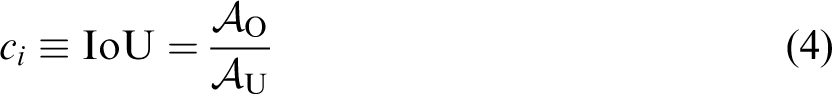
The class score s is computed by multiplying the conditional class probabilities and the individual confidence score for each landmark:

The best prediction is selected from the 49 predictions according to the highest class score
In the next subsection, we will comprehensively describe how to optimize the learnable parameters
Training the convolutional neural network on a GPU workstation
For training the CNN detection framework, we first resize the input image into 224 × 224 and then divide it into a 7 × 7 equally-sized grid cells. The cells are responsible for detecting the landmark if the center of the landmark falls into one of them. As described in the previous subsection, the CNN framework generates a
The loss function consists of three parts, i.e. the area loss 


The overall loss function is:

Given a batch of training data (m image samples), we train the detection model via the stochastic gradient descent (SGD) algorithm. We first initialize the learnable weights W and biases b to a small random value near to zero subject to a normal distribution –

Set 1. Compute the gradients 2. Set 3. Set
Update the parameters:

To train the CNN based detection model, we repeatedly take steps of the stochastic gradient descent as described in Algorithm 1 to minimize the loss function
There are two things that need to be noted in our training procedure. First, the data jittering approach is employed to augment the landmark dataset. Specifically, the augmentation strategies operated on the landmark dataset include adjusting the image exposure, saturation and hue. The data augmentation increases the intraclass variability of training data and thus further improves the robustness of the detection model. Second, the training is carried out on a Graphics Processing Unit (GPU) work station, which is widely used for training deep learning models. However, it is not suitable for an MAV on-board system to perform CNN training by involving GPUs, which are normally physically big in size and comparatively power consumptive. On the other hand, it is not necessary to train a CNN in an on-board system because the MAV instant manipulation just requires implementing a trained CNN model rather than training it. In the light of this observation, we use an off-board GPU workstation for efficiently training our CNN framework. After the training procedure, we obtain about 4000 optimal parameters, i.e. optimal weights
Landmark detection based on the trained convolutional neural network
Landmark detection via CNN inference
The training procedure first forwardly computes the prediction tensor based the initial parameter values, and then adjusts the parameter values backwardly via back propagation optimization. In contrast to the forward-backward training procedure, the inference procedure processes each frame of a captured video through the CNN network only forwardly, based on the optimal parameter values (weights
Set L = 5, 1. (a) Set K = Ks(l). (b) 2. Process feature maps in the layer FC1 based on 3. Process feature maps in the layer D1 based on 4. Compute the class score s for each prediction according to equation (5). 5. Select the best coordinate prediction


Implementing detection on an MAV on-board system
We implement the detection model on the MAV on-board system Manifold, which consists of a quad-core ARM Cortex-A15 processor and 2 GB memory. The trained network is used for detecting landmarks from unlabeled video frames captured by the on-board camera. To run the inference procedure on Manifold, we build detection model with the 4000 optimal parameters (
It should be noted that we train and implement the CNN detection framework based on separate hardware platforms, i.e. the GPU workstation and the Manifold MAV on-board system. Though the CNN framework is developed with simplified architecture, it still requires considerable computational overheads especially in the training phase. Specifically, inferencing with the trained CNN is much less computational consumptive than training it, because the inference implementation does not involve the costly backward gradient computation. Therefore, in contrast to exploiting the computational power of the GPU workstation to handle the complex computation in the training phase, we implement the less complex detection procedure in the Manifold MAV on-board system, which is not only smaller in size, lighter in weight and less costive in power than the GPU workstation but also qualified to conduct an on-line real-time landmark detection.
Landing system
Figure 4 illustrates the operating procedures of the autonomous landing system. The image acquisition procedure is completed by capturing video frames using an on-board camera with universal serial bus (USB). The coordinates of the landmarks are predicted by forwarding the trained CNN detection model. The predictedcoordinates of the landmarks are then converted into x-axis and y-axis angular offsets (in radians) of the landmark center. These angular offsets are sent to the autopilot via the Micro Air Vehicles Communication Protocol (MAVLINK). This information is used to generate control signals to supervise the landing process via the autopilot. The detailed procedures are described in the following subsections.
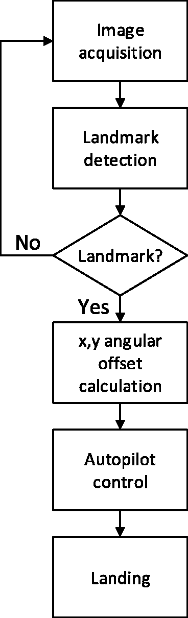
The flow chart of the vision-based MAV landing system.
Software architecture
The predicted landmark coordinates from videos captured by an MAV on-board camera are transformed to the MAV's own coordinates. We assume that the roll, pitch and yaw angles of the MAV can be neglected while computing the x-axis and y-axis angular offsets of the landmark coordinates in images. The x-axis and y-axis angular offsets are obtained as follows:
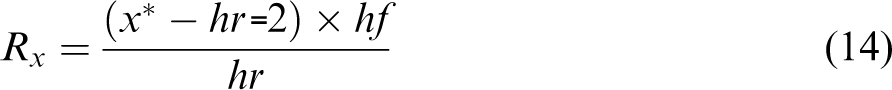

Here
The Rx and Ry are sent to the autopilot as MAVLINK message. This information is processed with sonar data to compute landmark position relative to the MAV.


A Kalman filter is then exploited for supervising the landmark, with the state vector defined as 


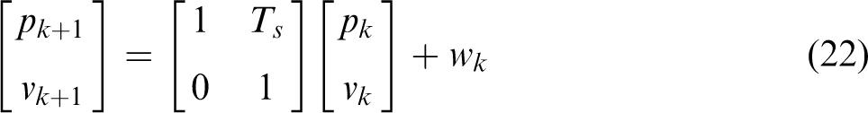
Assume that the modeling noise wk is white zero-mean Gaussian noise with a covariance matrix Q, and the measurement noise uk is white zero-mean Gaussian noise with a covariance matrix R:


The state propagation and update equations for the Kalman filter are summarized as follows.
The predicted state estimation is:
The predicted estimation covariance is:
The innovation covariance is:
The optimal Kalman gain is:
The updated state estimation is:
The posterior covariance is:


In this group of equations, the superscript T indicates matrix transposition,
The position and velocity estimate
Hardware architecture
The hardware architecture is shown in Figure 5. In this system, we develop a customized do-it-yourself (DIY) quad-rotor with an embedded development board (Manifold). As the main processing unit, the Manifold board carries out the following tasks: (1) processing all images captured by the on-board camera; (2) calculating the angular offset; (3) communicating with the autopilot. The communication between the Manifold and the MAV main body is enabled by the Dronekit.

Hardware architecture of the vision-based autonomous landing system.
In our system, the Manifold connects to the UAV's autopilot through USB TTL Serial cables. The baud rate of the serial connection is 1,500,000, and the MAVLINK is used for communication. The Dronekit API is utilized as the development tool for our system.
The experimental quadrotor is shown in Figure 6, with a DJI NAZA F450 X-shaped frame and the Pixhawk autopilot with ArduPilot Firmware. Pixhawk integrates a 14 bit accelerometer, a 16 bit gyroscope, a magnetometer and an MS5611 barometer. A sonar is used to measure the height of the MAV above the ground. A USB camera is used to detect the landmark. The camera and sonar are configured as shown in Figure 7. The key component of the UAV's computing system is the Manifold, which consists of a quad-core ARM Cortex-A15 processor and 2 GB memory.

The developed DIY quadrotor (from the top view of the MAV).

The configuration of camera and sonar (from the bottom view of the MAV).
Experimental results
In the experiments, we use five categories of landmarks (as shown in Figure 1) for testing the performance of our framework. The landmarks size is 50 cm × 50 cm. The MAV with a downward looking camera is used to capture outdoor videos, and the flying height varies from 1 m to 5 m. We also use a forward looking camera for the MAV to capture indoor videos. The captured videos are separated into image frames. In order to train our model to be robust with respect to inconsistent lighting, we intentionally change image brightness and thus obtain various lighting training data. The brightness value ranges from 0 representing complete darkness to 100 representing complete whiteness. In our training process, the brightness values of 50 images from each landmark category are set to be 10, and those of another 50 images from each landmark category are set to be 90. We also use the data augmentation strategy presented in the previous section to enlarge the intraclass variability of the training data for the purpose of training a comprehensive model.
The images for each landmark category are annotated by using an open source tool – labelImg 1 https://github.com/tzutalin/labelImg. An obtained annotation file includes the category names and landmark coordinates. We build a training dataset containing images and their annotations. In our experiment, 200 images for each of the five landmark types are used to train our landmark detection model and the training data contains totally 1000 annotated images. The training process is realized on a workstation with a NVIDIA GTX860M GPU.
The values of IoU of our CNN model are shown in Figure 8. The IoU value reaches the peak after 35,000 iterations. We choose the CNN model with 35,000 iterations during the training procedure as our landmark detection model.
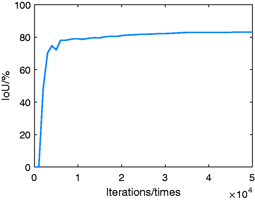
The values of IoU with different iterations.
In order to empirically evaluate the proposed on-board CNN-based landmark detection model, we use the test data sets, which are different from the training data sets, for testing our trained model. Specifically, we perform experiments on the Manifold board, which processes the outdoor and indoor real-time video frames as test data sets. Four tests are carried out:
In the first set of experiments, we evaluate the robustness of the detection model for various landmark shapes. In the second set of experiments, we evaluate the robustness of the detection model for different illumination intensities. In the third set of experiments, we evaluate the robustness of the detection model for different background environments. In the fourth set of experiments, we evaluate the efficiency of the detection model.
Evaluation of the robustness of the detection model for various landmark shapes
To evaluate the effectiveness of our model for detecting various landmark shapes, we test our CNN model in terms of detecting each type of landmarks in 1000 images captured by the MAV camera. Results for the five landmarks are shown in Figure 9 and Table 2. Our CNN model successfully recognizes the landmarks in 4973 frames. The T-shaped landmark is mistaken for the H-shaped landmark in several rotation frames. This is because both the T-shaped landmark and the H-shaped landmark are simply featured by less discriminative black lines, and we only use 200 images of each type of landmarks to train our model. The landmark composed of an H-shaped and concentric circles is mistaken for the H-shaped landmark in several frames. We observe that these errors occur when the distance between the camera and the landmark is large. One reason for the misidentification of the H-shaped and circle landmarks is that they are symmetric shapes and are less distinguishable from distant views. To validate this observation, we use a fake target landmark, which appears similar to the circle landmark but is asymmetric, to replace the circle landmark for testing our model (Figure 9(f)). The experimental result reveals that our model does not misidentify the fake landmark as the true landmark. Our detection model can distinguish the landmark composed of a series of concentric circles and the fake targets from distant views correctly.

Landmark detection results: (a) the T-shaped landmark; (b) the H-shaped landmark; (c) the landmark consisting of eight equal-sized squares and a big white border; (d) the landmark composed of a series of concentric circles; (e) the landmark composed of an H-shaped and concentric circles; (f) the fake landmark.
Results for evaluating the detection model for various landmark shapes.

Qualitative evaluation results of the CNN model on the video frames captured from various flying heights and from different rotation angles are shown in Figure 10. The performance of our model is fairly stable when the MAV searching for the landmark at different heights and rotations. The processing rate is 21 frames per second.

Detection results of the detection model on video frames captured from various flight heights ((a), (b) and (c)) and from different rotation angles ((d), (e) and (f)).
To make the evaluation of the model robustness one step further, we use the MAV shown in Figure 6 to test the landing system with respect to different landmarks. The MAV takes off near the landmark to 4 m. When the landmark is detected, the vision-based landing system manipulates the MAV to autonomously land to the landmark region. All the actions in our test are performed by the MAV automatically. We test four flights for each landmark, and measure the horizontal distance between the MAV center to the landmark center in x and y axis. The position errors (ex and ey) are recorded in Table 3.
Position errors.

We can see from Table 3 that the position errors are acceptable for practical landing, because they are relatively small compared with the landmark size 50 cm × 50 cm. One reason for the position errors is that we assume the roll and pitch angles of the MAV to be zero during the MAV landing for the purpose of making condition controlled evaluations. This assumptive constraint causes some position measuring errors that do not arise from the detection model. Although suffering from these artificial errors, the MAV can still automatically land within the landmark region safely.
Evaluation of the robustness of the landmark detection model for different illumination intensities
In this set of experiments, 100 variously illuminated images for each landmark category are used for validation. Specifically, we generate different lighting situations by changing the brightness value of test images. The brightness values of the 100 images are set to be from 10 to 90 to test our landmark detection model. Visual results are shown in Figure 11. Experimental observations reveal that the detection results are stable for the MAV landmark navigation under various light conditions.

The detection results for the images with different brightness values: (a) the brightness value is 10; (b) the brightness value is 30; (c) the brightness value is 70; (d) the brightness value is 90.
Evaluation of the robustness of the landmark detection model for different background environments.
To make the empirical evaluation of our model one step further, we test the detection performance of our method for detecting landmarks in different backgrounds. Specifically, we perform experiments on the videos captured in four different background environments with the on-board camera. Two videos are captured outdoors, and the other two are captured indoors. We use 200 images captured in each environment to test our model. The results are shown in Figure 12 and Table 4. The experimental results validate that our landmark detection model is able to detect landmarks under various environments.
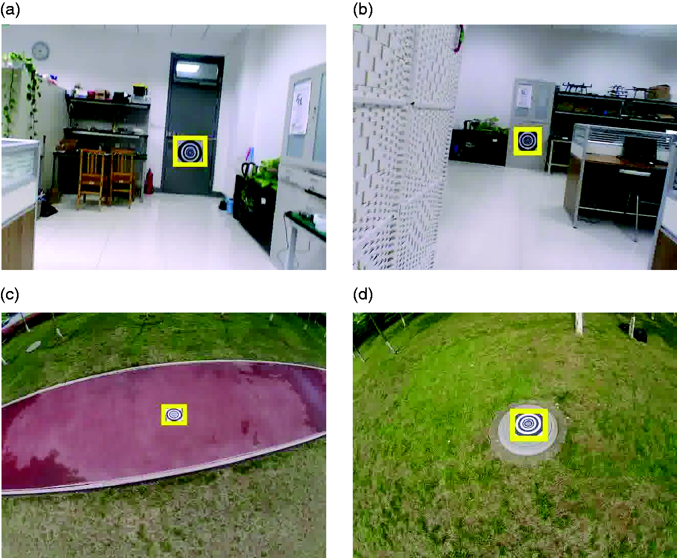
The landmark in various environments: (a) and (b) are indoor environments; (c) and (d) are outdoor environments.
Results for evaluating the detection model for different background environments.

Evaluation of the efficiency of the landmark detection model
To make a quantitative comparison between our method and alternative state-of-the-art methods, we train the tiny models of Yolo 17 and Yolo v2 18 based on the same training dataset as that of our model. We then test the three trained models in terms of average IoU and processing rate (i.e. processed frames per second). The experiments are performed based on the same image frames as those in the first set of experiments. The comparison results are shown in Table 5. We observe that though the Yolo methods are slightly better in terms of accuracy, our model is much more efficient. The MAVs usually have limited computing resources on board (e.g. Manifold), which make the Yolo methods hardly achieve real-time implementation. On the other hand, our model achieves efficient implementation, which enables practical MAV on-board computation.
Comparison in terms of accuracy and efficiency.
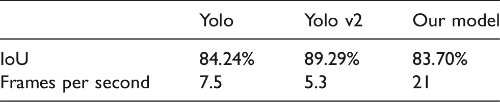
IoU: intersection over union.
The usage of the CPU and memory the detection procedure is reported in Table 6. The landmark detection image processing algorithms use 3/4 of computing resources. Therefore, it allows more accurate control algorithms to execute during the landing procedure, which provides a possible route for improving the landing accuracy.
CPU and memory usage. CPU: central processing unit.

These experiments validate that our CNN model can not only detect the various landmarks, but also produce correct detections under different conditions. We put the detection results in video forms on the URL https://youtu.be/fifCK6BeDH8 for public observation. It is clear that our method is robust and efficient to process landmark information for guiding the MAV autonomous landing.
Conclusions
We have introduced a novel vision guided MAV autonomous landing system based on deep learning. Specifically, we have made three novel contributions. First, we have incorporated a modified SqueezeNet architecture into the Yolo scheme to develop a simplified CNN for detecting landmarks. Second, we have designed a separative implementation strategy which leverages the complex CNN training and the instant CNN detection. We have tested our novel framework in both synthesized and real-world environments and validated its effectiveness for MAV autonomous landing.
Footnotes
Declaration of conflicting interests
The author(s) declared no potential conflicts of interest with respect to the research, authorship, and/or publication of this article.
Funding
The author(s) disclosed receipt of the following financial support for the research, authorship and/or publication of this article: This work was supported by National Natural Science Foundation of China (Grant No.: 61671481 and 61701541), Shandong Provincial Natural Science Foundation(Grant No.: ZR2017QF003), Qingdao Applied Fundamental Research Project (Grant No.: 16-5-1-11-jch), the Royal Society of Edinburgh and National Natural Science Foundation of China joint project 2017-2019 (Grant No.: 6161101383) and the Fundamental Research Funds for Central Universities(Grant No.:15CX05042A and 16CX05004B).