Sage Journals: Discover world-class research

Abstract

The radiofrequency identification (RFID) technology is widely used in modern industry to identify and localize the final manufactured products and their parts. This article analyses and optimizes the localization process of special RFID transponders – markers used to mark the position and type of the underground facility networks (pipes, cables, etc.). The analysis of electric circuits representing the system consisting of the marker and the localization device is performed by numerical solution of the corresponding equations. The results of the numerical solution are then used for calculation of the analytical description of the waveform received as response from the excited marker. The constants obtained from the analytical form of the solution are then used as input parameters for optimization of time window width in the correlation receiver of the marker responses. The optimization is focused on the maximization of the signal-to-noise ratio in the receiving time window. The theoretical calculations are completed by the processing of real signals recorded by an oscilloscope from the localization device where the correlation receiver is planned to apply.

Keywords

Localization radiofrequency identification correlation receiver marker response noise

Introduction

The utilization of radiofrequency identification (RFID) transponders is widely applied in today’s industry applications. The transponders are used to identify and/or to localize various kinds of goods and other items. Special RFID transponders are being used to mark the position of the underground facility networks such as telecommunication and energetic cables or water and gas pipes – such transponders are called markers and they are used especially in the case when the underground pipelines are manufactured from the plastic material or when the optical cables are used (without metal conductor). The markers are buried under the ground surface near the marked facility, especially at the important points of the underground facility, that is, crossing with other cables/pipes, connectors, branches, and so on.

The markers are single-bit RFID transponders¹ consisting of tuned LC circuit. The working frequencies of the markers are in the low frequency (LF) band (77–170 kHz), and they depend on the type of the underground facility, for example, 83.0 kHz markers are being used for the gas pipes, 101.4 kHz for the telecommunication cables and so on up to 169.8 kHz for energetic cables. The localization process of the markers with unknown position under the ground surface is based on searching maximum response from the marker by the localization device manually moved in terrain by the operator, so the localization is based on the very popular Received Signal Strength Indication (RSSI) method, which is widely adopted not only in the RFID application but also in the localization using ambient radio transmitters.²

The antenna of the localization device is inductively coupled with the marker and this fact causes some negative properties of localization process, especially very rapid fall of the marker response amplitude with increasing distance between the marker and the localization device. The response amplitude is inversely proportional on the sixth power of the distance,³ so the markers must be buried in depth no more than 1.5–2 m. This is a very limiting factor for the signal receiver in the localization device, especially due to the noise, and therefore, this article describes an analysis of the localization process and optimization of the correlation receiver adapted for receiving the responses from the markers.

The theory of the correlation receiver was developed for additive white Gaussian noise (AWGN) channels and for constant modulation rate, that is, for constant duration of the received symbols.⁴ Then, the correlation receiver based on the bank of correlators or on the bank of matched filters works on the maximum likelihood principle. But in the case of the marker localization, the received marker response is in fact the symbol with theoretically unlimited duration because the response is essentially a damped sine wave signal with attack and decay time constants, so the duration of the receiving time window must be calculated taking the maximization of signal-to-noise ratio (SNR) into account.

Related works

The localization of the RFID transponders is an actual research topic today. The basic review of RFID transponder localization techniques is given in the study by Sanpechuda and Kovavisaruch.⁵ Most of the research studies deal with the localization of the transponders in the ultra high frequency (UHF) band where propagation of the electromagnetic waves is different from propagation of the waves in the LF band. Therefore, the approaches described in the studies by Han et al.⁶, Alsalih et al.⁷ and Ting et al.⁸ are applicable to the UHF RFID transponder localization, and they are based on the intersection of multiple RFID reader ranges or on radio maps composed of multiple points, so the localization of underground RFID transponders in terrain by these methods would be impractical. The RSSI-based localization of the UHF RFID transponders is described in the study by Zhang et al.,⁹ in which a relationship between the RSSI value and the transmission power of the reader is analyzed. The segmented antenna system used for localization of small animals is designed in the study by Catarinucci et al.¹⁰ The transponders used for this application work in the UHF band but small localization distances in this case enable that the system uses near field of the segmented antenna.

Similar application to that described in this article is introduced in the study by Daly et al.,¹¹ in which the RFID markers are embedded in concrete and they serve as way points in warehouses. For this purpose, the transponders in the UHF band (868 MHz) were selected as the most suitable, and they were tested with standard and redesigned antennas. The LF band markers were evaluated as unsuitable for this application due to their higher dimensions. Another application of the RFID transponder localization where the transponders are static is described in the study by Ota et al.¹² In this article, the microwave transponders (2.45 GHz) are used and the localization reader is moved by a mobile robot. To evaluate the position of the transponder, an adaptive likelihood model of reader read range is used. In the study by Liu et al.,¹³ the static transponder is localized by the reader which is moved in two axes above the plane where the transponder is placed. This approach enables to calculate the position accurately by moving the reader around the transponder position.

In the LF band, the coupling between the marker and the antenna of the localization device can be modelled by mutual inductance. Because both the marker and the localization device antenna are coupled resonant LC circuits, the theoretical analysis in the study by Cohen¹⁴ gives good introduction to the mathematical analysis of the marker localization problem. Similar analyses are provided in the studies by Gurleyuk et al.¹⁵ and Abbasi and Khanzade,¹⁶ in which the Tesla transformer is analyzed in frequency and time domains.

The correlation receiver and/or matched filter applications in the RFID technology are described in many sources. Brandl et al.¹⁷ described a special RFID transponder equipped with a chirp signal generator which transmits the chirp signal into the base stations where the matched filters are used to obtain chirp signal autocorrelation function. The position of the RFID transponder is then estimated by the time of arrival (ToA) method. The matched filter is also applied for baseband data demodulation in the UHF RFID reader working with EPCglobal Class-1 Gen-2 RFID transponders.¹⁸ Such robust data demodulator allows compensation of signal distortion and frequency deviation. In the study by Amin et al.,¹⁹ the novel digital-matched filter without adders is described and applied to demodulation of signals spread by the Barker code, which is being used in IEEE 802.11 compatible RFID transponders. Another application of the correlation receiver is proposed in the study by Liu et al.,²⁰ in which the digital correlation demodulator for the UHF RFID reader can work with a low SNR. Similar digital receiver architecture for demodulation of low SNR signals from the UHF RFID transponders is proposed in the study by Angerer.²¹ Xi and Cho²² demonstrated lower bit error ratio in comparison to the traditional RFID decoder when the matched filter in the decoder is used. The problems with noise in UHF RFID are studied in the study by Blažević et al.,²³ in which the authors measure a distribution of SNR by using a software-defined radio receiver.

The correlation receiver and/or the matched filter is applied not only in the RFID technology but also in many other areas of the communication systems such as the radiolocation and the mobile communications. The reduction in noise by the matched filter is described in the study by Islam and Chong,^24,25 but in these papers the main application is focused on the pulse and continuous wave radars. The authors performed comparison of the matched filter and the wavelet transformation properties in noise reduction. Similar problems are solved in the study by Sarkar and Pal,²⁶ in which the matched filter is applied to reduce the noise in the pulse radar.

In the study by Slock and Trigui,²⁷ the interference cancelling matched filter is analyzed for application in mobile communication where the interferences are considered as interference generated by multiple channel users mixed with Gaussian noise. The optimal selection of the integration time in the ultra-wideband (UWB) correlation receiver is solved in the study by Chao.²⁸ The optimization in this case is focused on calculation of minimal bit error probability of the used correlation receiver. In the study by Chao,²⁸ the similar optimization problem to that in this article is solved, but the difference is in the shape of the received signal – in the study by Chao,²⁸ the power of the received signal decays exponentially, the received marker response which is analyzed in the next chapter has both exponential attack and decay.

Mathematical model of the localization device – marker system and its solution

This model is based on the models which the authors published previously in the studies by Vestenický et al.^29,30 These older models were solved only numerically, and they were used only to obtain the dependence of the marker response amplitude on the distance between the marker and localization device and on the marker resonant frequency. Note that the model in the study by Vestenický et al.²⁹ is simplified and it does not contain the damping resistance and time interval. The model described here is extended by the analytical solution of the marker response waveform which is in next chapters used for optimization of the marker response receiving window width and for comparison of the Simulink model output.

The process of the marker localization is illustrated in Figure 1. The marker is modelled as a serial resonant circuit with parameters R_T (loss resistance), L_T (inductance) and C_T (capacitance), and the antenna of the localization device is modelled similarly with parameters R_R, L_R and C_R. The localization process is divided into three time intervals as follows:

Marker excitation, 0 ≤ t < T₁, when the switch SW1 is in position 0;

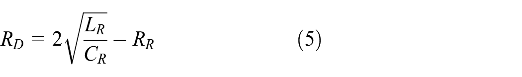
Damping of the antenna self-oscillation, T₁ ≤ t < T₂, when the switch SW1 is in position 1 and the switch SW2 is in position 0, the damping resistor RD is calculated from equation (5); and

Receiving of the marker response, t ≥ T₂, when the switch SW1 is in position 1 and the switch SW2 is in position 1. In this time interval, the antenna current is measured by the current sensing resistor R_S.

Figure 1.

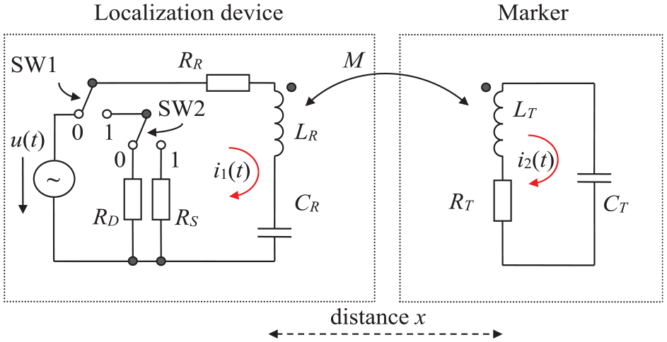
Electrical circuit representing principle of the marker localization process.

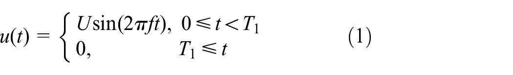
The marker is excited by a harmonic generator with amplitude U and frequency f described by equation (1), M is the mutual inductance between the marker and antenna coils given by equation (2), where µ₀ is the permeability of vacuum, N_R and N_T are the number of antenna and marker coil turns, r_R and r_T are the radiuses of the coils and x is the distance between the antenna and the marker. Note that equation (2) is approximative, and it assumes that the coils have common axis

u (t) = {\begin{matrix} U \sin (2 π ft), 0 \leq t < T_{1} \\ 0, T_{1} \leq t \end{matrix}

(1)

M = \frac{π μ_{0}}{2} \frac{N_{R} N_{T} r_{R}^{2} r_{T}^{2}}{{(r_{R}^{2} + x^{2})}^{3 / 2}}

(2)

The currents i₁(t) and i₂(t) in Figure 1 can be calculated by the loop current method from the system of equation (3). The resistor R is varying and its value is changed in accordance to equation (4) in every of the three time intervals. To obtain solution, the second-order system (3) was transformed into the first-order system by the substitution of x₁(t) = i₁(t), x₂(t) = di₁(t)/dt, x₃(t) = i₂(t) and x₄(t) = di₂(t)/dt, which is given by equation (6)

\begin{matrix} L_{R} \frac{d^{2} i_{1} (t)}{d t^{2}} + R \frac{d i_{1} (t)}{dt} + \frac{i_{1} (t)}{C_{R}} - M \frac{d^{2} i_{2} (t)}{d t^{2}} = \frac{du (t)}{dt} \\ L_{T} \frac{d^{2} i_{2} (t)}{d t^{2}} + R_{T} \frac{d i_{2} (t)}{dt} + \frac{i_{2} (t)}{C_{T}} - M \frac{d^{2} i_{1} (t)}{d t^{2}} = 0 \end{matrix}

(3)

R = {\begin{matrix} R_{R}, 0 \leq t < T_{1} \\ R_{R} + R_{D}, T_{1} \leq t < T_{2} \\ R_{R} + R_{S}, T_{2} \leq t \end{matrix}

(4)

R_{D} = 2 \sqrt{\frac{L_{R}}{C_{R}}} - R_{R}

(5)

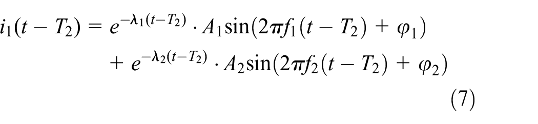
System (6) is nonhomogeneous only in the first time interval (marker excitation), so the solution in the third interval (marker response receiving) where system (6) is homogeneous can be easily obtained in analytical form. The analytical solution is based on the eigenvalues and the eigenvector calculation of the system matrix in equation (6), and the resulting waveform of the current i₁(t) in the antenna coil during the third time interval is described by equation (7), that is, the received response of the marker is composed of two damped harmonic waveforms. It is in conformance with the conclusions in the study by Cohen.¹⁴ The parameters in equation (7) were calculated from the general solution of system (6). The initial conditions, which are necessary to obtain the final solution of system (6), were taken from the numerical solution in time interval <0, T₂) because the analytical solution of system (6) in whole time interval <0, ∞) is complicated due to inhomogeneity of system (6) in the initial time interval <0, T₁).

The damping factors λ₁ and λ₂, frequencies f₁ and f₂ and phase shifts φ₁ and φ₂ in equation (7) were calculated for input parameters given in Table 1

\begin{matrix} (\begin{matrix} \frac{d x_{1} (t)}{dt} \\ \frac{d x_{2} (t)}{dt} \\ \frac{d x_{3} (t)}{dt} \\ \frac{d x_{4} (t)}{dt} \end{matrix}) = (\begin{matrix} 0 & 1 & 0 & 0 \\ \frac{L_{T}}{C_{R} (M^{2} - L_{R} L_{T})} & \frac{L_{T} R}{M^{2} - L_{R} L_{T}} & \frac{M}{C_{T} (M^{2} - L_{R} L_{T})} & \frac{M R_{T}}{M^{2} - L_{R} L_{T}} \\ 0 & 0 & 0 & 1 \\ \frac{M}{C_{R} (M^{2} - L_{R} L_{T})} & \frac{MR}{M^{2} - L_{R} L_{T}} & \frac{L_{R}}{C_{T} (M^{2} - L_{R} L_{T})} & \frac{L_{R} R_{T}}{M^{2} - L_{R} L_{T}} \end{matrix}) \cdot \\ (\begin{matrix} x_{1} (t) \\ x_{2} (t) \\ x_{3} (t) \\ x_{4} (t) \end{matrix}) + (\begin{matrix} 0 \\ \frac{L_{T}}{L_{R} L_{T} - M^{2}} \cdot \frac{du (t)}{dt} \\ 0 \\ \frac{M}{L_{R} L_{T} - M^{2}} \cdot \frac{du (t)}{dt} \end{matrix}) \end{matrix}

(6)

\begin{matrix} i_{1} (t - T_{2}) = e^{- λ_{1} (t - T_{2})} \cdot A_{1} \sin (2 π f_{1} (t - T_{2}) + φ_{1}) \\ + e^{- λ_{2} (t - T_{2})} \cdot A_{2} \sin (2 π f_{2} (t - T_{2}) + φ_{2}) \end{matrix}

(7)

Table 1.

Parameters of the mathematical model.

Quantity	Value
N_r	37
N_t	37
T ₁	1.233 ms
T ₂	1.272 ms
R_S	1 Ω
L_R	925.16 µH
L_T	925.16 µH
C_R	2.663 nF
C_T	2.663 nF
R_D	1168.9 Ω
R_R	9 Ω
R_T	6.549 Ω
F	101.4 kHz
U	12 V

The dependencies of the parameters λ₁ and λ₂, f₁ and f₂, A₁ and A₂ and φ₁ and φ₂ on the distance x between the antenna and the marker are illustrated in the series of the next figures. The parameters of the marker response waveform can be considered as constant for the distances greater than approximately 0.7 m except the amplitudes A₁, A₂, which fall rapidly with the increase in distance. Then, we can consider that the amplitudes A₁=A₂, frequencies f₁=f₂ and phase shifts φ₁ = 0°, φ₂ =−180°, so that equation (7) can be simplified into the following form

i_{1} (t - T_{2}) = (e^{- λ_{1} (t - T_{2})} - e^{- λ_{2} (t - T_{2})}) \cdot A_{1} \sin (2 π f_{1} (t - T_{2}))

(8)

The simplified equation (8) represents the case which occurs under normal operating conditions during the marker localization process because the markers are usually buried in depth approximately 1 m. The damping factors λ₁ and λ₂ in this case converge to the damping factors of separated resonant circuits of the marker and the antenna, see equation (9), where Q_T is the quality factor of marker resonant circuit and ω = 2πf (Figures 2 and 3). Similar calculation is valid for λ₂

λ_{1} = \frac{R_{T}}{2 L_{T}} = \frac{ω}{2 Q_{T}}

(9)

Figure 2.

Dependence of the damping factors (a) and the frequencies of the received marker response on distance (b).

Figure 3.

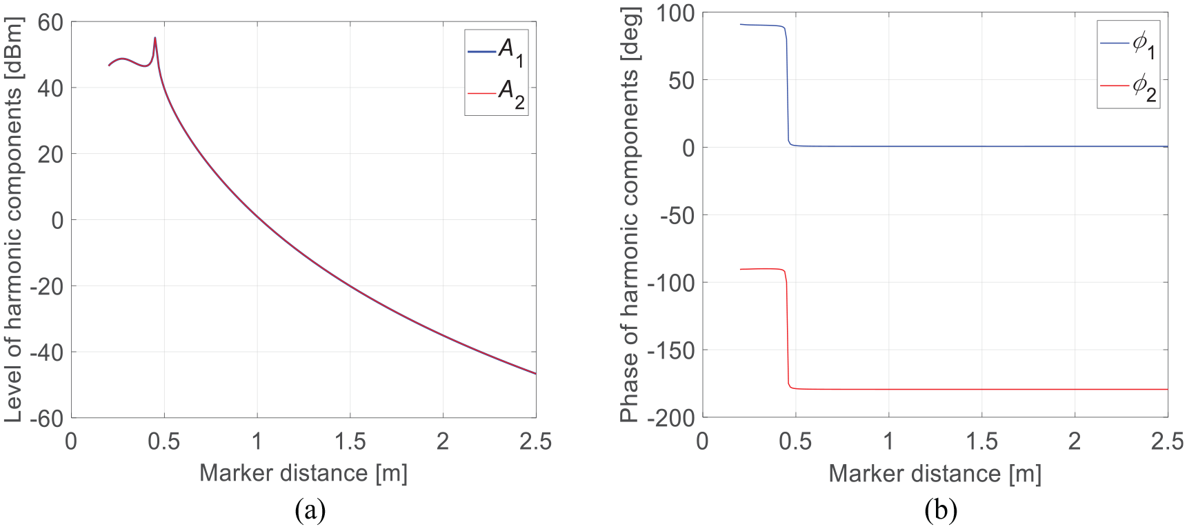
Dependence of the amplitudes (a) and the initial phase shifts of on distance (b).

Simulink model of the localizationdevice – marker system and its evaluation

The model of the system presented in Figure 4 was build up in Simulink environment to enable the simulation of the noisy marker responses and compare the ‘pure’ marker responses to the solution given by equation (7). The proposed model is based on the electrical circuit presented in Figure 1 and supplemented by auxiliary blocks that enable the correct circuit excitation, the time interval switching and export of resulting waveforms to the MATLAB workspace. The white noise source ‘White Noise’ block along with the bandpass filtering block ‘Bandpass filter’ were added to the model to produce noisy marker responses. The coils of the resonant circuits are modelled by the ‘Lr_Lt’ block, with three parameters – inductances of the coils (L_R, L_T) and the coupling factor k given by equation (10)

k = \frac{M}{\sqrt{L_{R} L_{T}}}

(10)

Figure 4.

Simulink model.

The antenna–marker system excitation is accomplished by product of harmonic carrier with frequency f = 101.4 kHz and amplitude U = 12 V generated by the ‘Carrier’ block and binary modulation signal generated by the ‘Modulation’ block. This signal controls the ideal voltage source ‘Modulated carrier voltage source,’ which drives the antenna serial resonant circuit. The modulation signal has the amplitude of 1 in the time interval < 0, T₁) and 0, otherwise. The damping resistor of the antenna circuit and its serial resistance are modelled through voltage controlled resistor ‘RD’ block, which is controlled by another binary signal generated by the ‘Damping’ block. The damping signal has the value of R_D given by equation (5) in the time interval < T₁, T₂) and 0, otherwise. Correct R_R value in the time intervals <0, T₁), < T₂, ∞) is given by the minimum resistance parameter in the ‘RD’ block with assumption that R_S = 0 Ω. There are three parameters of the white noise source block: mean value N_M = 0, variance N_V and random generator seed S which is set to a random number for each run of the simulation. The properties of the filtered noise are determined by the frequency response of used band pass filter in terms of frequency dependence of power spectral density (PSD) and variance parameter N_V in terms of its average power. The parameters of the bandpass filter block were determined in such a manner that the PSD characteristic of generated noise and the PSD characteristic of noise sampled in real localization device are approximately matched (Figure 5). Note that the interferences from the local (unknown) source and from the telemetric transmitter located in Lakihegy, Hungary (135.6 kHz) were omitted. The variance parameter was determined in the manner so that the average powers of both noises are equal. The currents in the circuit loops are measured through the ideal ampere metre ‘I_ANT’ and ‘I_MKR’ blocks. The physical components L_R, C_R, R_R, R_D, L_T, C_T and R_T are modelled by Simscape blocks and therefore they need to use conversion blocks between the Simulink and Simscape signals, ‘S-PS#x’ and ‘PS-S#x’, respectively. The resulting waveforms are exported to the MATLAB workspace by the ‘To Workspace x’ blocks. The antenna current i₁(t) is exported through the ‘To Workspace 3’ block, the marker current i₂(t) is exported through the ‘To Workspace 1’ block and the filtered noise signal and noisy antenna current are exported through ‘To Workspace 2’ and ‘To Workspace’ blocks, respectively.

Figure 5.

PSD of real and simulated noise.

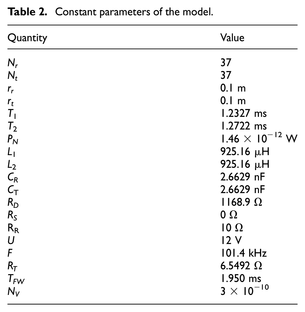
The resulting waveform of i₁(t) obtained from the Simulink model was evaluated against the waveform obtained from equation (7). Both models were fed with equal parameters according to Table 2. The resulting waveforms for selected marker distances (1.2 and 1.65 m) are presented in Figure 6(a), (c) and (b), (d) respectively. The difference between results from both models was evaluated as difference in envelopes of i₁(t) waveforms obtained from both models, and it is presented in percentage scale in Figure 7. It can be seen that the difference slightly increases in time. Peak values of the difference are present mainly for very small amplitudes of i₁(t) at the beginning and at the end of receive window. In the main portion of the receive window, the difference value is kept well below 0.5%. As we want to use i₁(t) to evaluate the correlations of noisy signals, this small difference can be neglected and both models can be assumed as equal.

Table 2.

Constant parameters of the model.

Quantity	Value
N_r	37
N_t	37
r_r	0.1 m
r_t	0.1 m
T ₁	1.2327 ms
T ₂	1.2722 ms
P_N	1.46 × 10⁻¹² W
L ₁	925.16 µH
L ₂	925.16 µH
C_R	2.6629 nF
C _T	2.6629 nF
R_D	1168.9 Ω
R_S	0 Ω
R_R	10 Ω
U	12 V
F	101.4 kHz
R_T	6.5492 Ω
T_FW	1.950 ms
N_V	3 × 10⁻¹⁰

Figure 6.

Antenna current i₁(t) for distance x = 1.2 m (a and c) and x = 1.65 m (b and d) obtained by analytical solution and simulation.

Figure 7.

Percentage difference of i₁(t) envelope for distance: (a) x = 1.2 m and (b) x = 1.65 m.

Theoretical relationship between the SNR and the correlation

Assuming the digital processing of the marker response waveform, the correlation receiver must have in its memory a set of calculated samples i₁(j) of the marker response i₁(t) as a reference signal. The noisy received signal will consist of the components mi₁(j), where m is a scale factor representing the decrease in the response with increased distance x and the noise component n(j). Then, the correlation coefficient Cor between the noisy and the reference signals can be calculated from the well-known Pearson formula

Cor = \frac{\sum_{j = 1}^{l} (m i_{1} (j) + n (j) - m \bar{i_{1}} - \bar{n}) \cdot (i_{1} (j) - \bar{i_{1}})}{\sqrt{\sum_{j = 1}^{l} {(m i_{1} (j) + n (j) - m \bar{i_{1}} - \bar{n})}^{2} \cdot \sum_{j = 1}^{l} {(i_{1} (j) - \bar{i_{1}})}^{2}}}

(11)

Assuming that the noise and the signal are statistically independent and that the mean values of the signal $\bar{i_{1}}$ and the noise $\bar{n}$ are zero, equation (11) can be simplified and the correlation coefficient Cor can be calculated from the next equation where SNR is the signal-to-noise ratio calculated from equation (13)

Cor = \sqrt{\frac{SNR}{SNR + 1}}

(12)

SNR = \frac{\sum_{j = 1}^{l} {(i_{1} (j))}^{2}}{\sum_{j = 1}^{l} {(n (j))}^{2}}

(13)

Optimization of receive window width

In accordance to equation (12), when we need to maximize the correlation between markers noisy response signal and the reference response signal we need to maximize the SNR. SNR can be expressed by equation (13) in the case that we have the discrete signals or by equation (14), if we have the signals defined analytically. Both equations are based on the energy of signal (E_S) and the energy of noise (E_N) ratio. In the case that we have analytically expressed the signal i₁(t), its energy E_S can be evaluated by equation (15) where τ is the upper integration boundary. It is obvious that the marker response signal can be seen in time interval <T₂, ∞) and therefore τ∈<T₂, ∞); moreover, it can be said that τ–T₂ is the receive window width parameter T_W according to equation (16). The energy of the noise E_N can be expressed by equation (17) in the case that the noise has constant average power

SNR = \frac{E_{s}}{E_{N}}

(14)

E_{s} = \int_{T_{2}}^{τ} i_{1}^{2} (t) dt

(15)

T_{W} = τ - T_{2}

(16)

E_{n} = (τ - T_{2}) P_{n}

(17)

Combining equations (7) and (15) new equation (18), which stands for energy of marker response over receive window width TW, can be obtained.

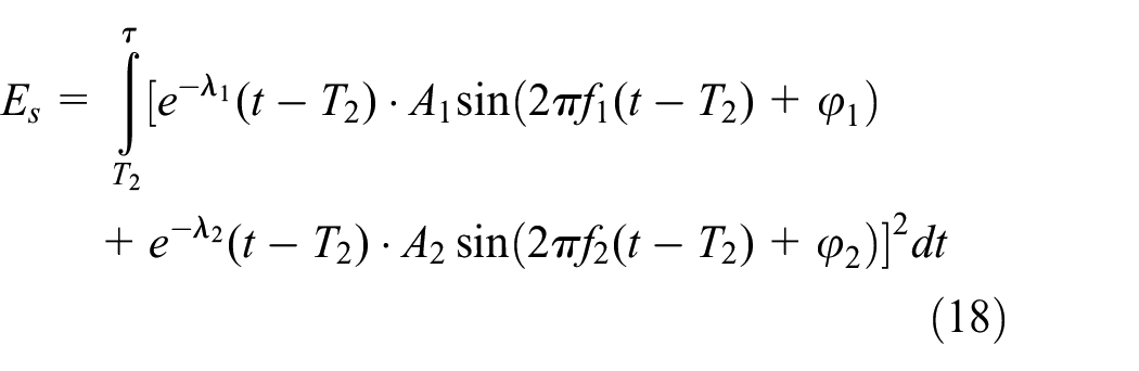
\begin{matrix} E_{s} = \int_{T_{2}}^{τ} [e^{- λ_{1}} (t - T_{2}) \cdot A_{1} \sin (2 π f_{1} (t - T_{2}) + φ_{1}) \\ + e^{- λ_{2}} (t - T_{2}) \cdot A_{2} \sin (2 π f_{2} (t - T_{2}) + φ_{2} {)]}^{2} dt \end{matrix}

(18)

The integral given by equation (18) can be easily evaluated for different parameters of the localization device–marker system and for various widths of the receive window T_W. Equation (18) was evaluated for the parameters summarized in Table 2 for selected marker distances and for receive window width T_W∈<0, 1.95> ms, and it is presented in Figure 8. It can be seen that the energy of signal is monotonically rising and asymptotically limited by upper bound and does not significantly rise with increase in the window width T_W beyond certain point. It is also clear that the energy of noise E_N given by equation (17) will increase linearly with increase in the window width T_W. The SNR dependency on window width T_W was evaluated for selected marker distances, and it is graphically presented in Figure 9. The SNR for each distance has a global maximum for certain value of T_WOPT.

Figure 8.

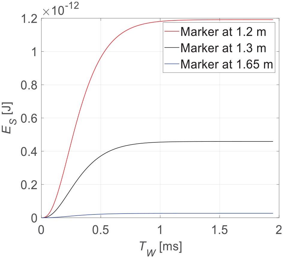
Energy of signal versus window width T_W.

Figure 9.

SNR versus window width T_W.

The evaluation of the SNR was performed for the marker distances from 0.2 up to 2.5 m for window width from 0 ms up to T_FW = 1.95 ms with a given time step of 1 µs. The corresponding T_WOPT value was found for each selected distance of marker by the MATLAB max function. The result of this process is presented in Figure 10. It can be seen that beyond certain distance the optimal window width remains practically constant. This phenomenon can be explained so that the damping factors λ₁ and λ₂ remain almost constant at the higher distances. The lower T_WOPT values for lower marker distances can be explained by the existence of the beats in i₁(t) waveform. The existence of the beats is evident because the frequencies of harmonic components in i₁(t) are not equal – refer to Figure 2(b). The SNR dependencies on marker distance for window width of T_WF and T_WOPT expressed in decibels are presented in Figure 11. The SNR values for optimized receive window width are 3–5 dB higher than the one for full window width. It can be supposed that this difference will increase the value of correlation between the noisy response signal and the reference response signal.

Figure 10.

Dependence of optimal window width on distance.

Figure 11.

Dependence of SNR on distance.

Conclusion

The optimization of the correlation receiver window width in marker localization is forced by a difference between the application of the correlation receiver in classical data transfer and the marker localization. The data transfer technologies usually use set of symbols representing the individual bits or groups of bits which have a constant duration given by inverse value of (constant) modulation rate. In the case of the marker localization, the response can be considered as a single symbol with theoretically infinite duration and considerably variable maximum amplitude dependent on marker distance. Therefore, the optimization of the receive window width is necessary to maximize the SNR.

To evaluate the optimization effect, the correlation between the noisy marker responses ‘I_ant’ and the reference response i₁(t) obtained from the Simulink model was evaluated according to equation (11) for both T_WF and T_WOPT window widths. The reference response was obtained from the Simulink model as a i₁(t) waveform evaluated at the marker distance of 0.6 m. The theoretical estimations of correlation based on SNR values according to equation (12) were also evaluated. The results are presented in Figure 12(a).

Figure 12.

Dependence of the correlations on the marker distance: (a) theoretical estimation versus simulation and (b) theoretical estimation versus real measurement.

Both the correlation curves obtained by the simulation and estimated from equation (12) for T_WOPT window width (orange and red curves) are significantly higher than those obtained for T_FW window width (magenta and blue curves). The correlation value is increased approximately by 0.2 for the marker distance 2.0 m after optimization. It can also be seen that the correlation values for both cases obtained from equation (12) are optimistic estimations. The increase in the correlation values for T_WOPT window width can be utilized in various ways. It can be used for the increase in the correlation threshold value to lower the probability of false marker detection preserving the detection distance or it can be used to extend the detection range preserving the correlation threshold value or the combination of both.

The results of the theoretical and simulation models were compared by the real experiment. In the experiment, the real signals from the marker localization device (an older model of the locator with an analogue signal processing by a phase-locked loop) were sampled by a digital storage oscilloscope with 1 Ms/s sample rate. This sample rate gives approximately 10 samples per period of the marker response signal (101.4 kHz) and such relatively slow sample rate was selected to try out the correlation receiver functionality when only small amount of RAM and CPU power will be usable in a planned battery-operated localization device. The marker responses were measured for marker distances from 0.3 up to 2.5 m with 0.1 m step and always 19 recorded consecutive time windows with the marker responses (such as in Figure 6) were used to calculate the correlation between the sampled signal and simulated response obtained from the Simulink model. The results together with the theoretical curves (for comparison) are presented in Figure 12(b) for a full receive window width and for optimized window width. The measured correlations (green and magenta curves) are slightly lower than theoretical values (red and blue curves) because in the received signal not only the noise but also the deterministic interferences are present (see the spectrum of the real signal, red curve in Figure 5). However, the benefit of the receive window width optimization is evident. For example, the measured correlation was increased by 0.2 from 0.45 up to 0.65 after optimization for marker distance 2.0 m. This corresponds to the increase in SNR by approximately 4.5 dB in accordance to equation (12).

Footnotes

Handling Editor: James Brusey

Declaration of conflicting interests

The author(s) declared no potential conflicts of interest with respect to the research, authorship and/or publication of this article.

Funding

The author(s) disclosed receipt of the following financial support for the research, authorship and/or publication of this article: This work has been supported by the grant of Cultural and Educational Grant Agency of the Slovak Republic (KEGA) No. 038ŽU-4/2017: ‘Laboratory education methods of automatic identification and localization using radiofrequency identification technology’.

ORCID iD

Peter Vestenický

References

Finkenzeller

. 2010 RFID handbook: fundamentals and applications in contactless smart cards, radio frequency identification and near-field communication. 3rd ed. Chichester: John Wiley and Sons.

Brída

Machaj

Benikovský

, et al. An experimental evaluation of AGA algorithm for RSS positioning in GSM networks. Electron Elect Eng 2010; 104(8): 113–118.

Vestenický

Mravec

Vestenický

. Comparison of various marker localization methods. In: Grzenda

Awad

Furtak

, et al. (eds) Advances in intelligent systems and computing: advances in network systems, vol. 461. Cham: Springer, 2017.

Proakis

Salehi

. 2008 Digital communication. 5th ed. New York: McGraw-Hill.

Sanpechuda

Kovavisaruch

. A review of RFID localization: applications and techniques. In: Proceedings of 5th international conference on electrical engineering/electronics, computer, telecommunications and information technology, ECTI-CON 2008, Krabi, Thailand, 14–17 May 2008, pp.769–772. New York: IEEE.

Han

Zhao

Cheng

, et al. Improving accuracy for 3D RFID localization. Int J Distrib Sens N 2012; 8(5): 865184.

Alsalih

Alma’aitah

Alkhater

. RFID localization using angle of arrival cluster forming. Int J Distrib Sens N 2014; 10(3): 269596.

Ting

Kwok

Tsang

AHC

, et al. The study on using passive RFID tags for indoor positioning. Int J Eng Bus Mana 2011; 3(1): 45678.

Zhang

Akré

Baey

, et al. Towards localization of RFID tags based on experimental analysis of RSSI. In: Proceedings of IFIP wireless days (WD), Rio de Janeiro, Brazil, 12–14 November 2014. New York: IEEE.

10.

Catarinucci

Colella

Mainetti

, et al. Near field UHF RFID antenna system enabling the tracking of small laboratory animals. Int J Antenn Propag 2013; 2013: 713943.

11.

Daly

Melia

Baldwin

. Concrete embedded RFID for way-point positioning. In: Proceedings of IPIN 2010, international conference on indoor positioning and indoor navigation, Zürich, 15–17 September 2010. New York: IEEE.

12.

Ota

Hori

Onishi

, et al. Localization of passive RFID Tags with robot using adaptive likelihood distribution algorithm. In: Proceedings of ATNAC 2007, Australasian telecommunication networks and applications conference, Christchurch, New Zealand, 2–5 December 2007, pp.163–168. New York: IEEE.

13.

Liu

Qiu

Yin

, et al. RILS: RFID indoor localization system using mobile readers. Int J Distrib Sens N 2018; 14(8): 155014771877128.

14.

Cohen

. The theory of coupled circuits (Classic reprint). London: Forgotten Books, 2017.

15.

Gurleyuk

Ozturk

Taskin

. Frequency domain analysis of Tesla transformer as a coupled second order system. Int J Appl Electrom 2011; 36(3): 207–215.

16.

Abbasi

Khanzade

. Analysis of dual resonant solid state Tesla transformer. Int J Mod Eng Res 2013; 3 (6): 3456–3460.

17.

Brandl

Posnicek

Kellner

. Position estimation of RFID-based sensors using SAW compressive receivers. Sensor Actuat A-Phys 2016; 244: 277–284.

18.

Jin

Cho

. A robust baseband demodulator for ISO 18000–6C RFID reader systems. Int J Distrib Sens N 2012; 8(9): 406710.

19.

Amin

Reaz

MBI

Jalil

. Design of a novel adder-less Barker matched filter for RFID. Int J Circ Theor App 2014; 42(3): 321–329.

20.

Liu

Huang

Min

, et al. Digital correlation demodulator design for RFID reader receiver. In: Wireless communications and networking conference, Kowloon, China, 11–15 March 2007, pp.1666–1670. New York: IEEE.

21.

Angerer

. A digital receiver architecture for RFID readers. In: International symposium on industrial embedded systems, Le Grande Motte, 11–13 June 2008, pp.97–102. New York: IEEE.

22.

Cho

. A RFID decoder using a matched filter for compensation of the frequency variation. In: 5th International conference on wireless communications, networking and mobile computing, Beijing, China, 24–26 September 2009, pp.1–5. New York: IEEE.

23.

Blažević

Solic

Škiljo

, et al. Signal-to-noise ratio measurements and statistical characterization in Gen2 RFID. In: 2nd International multidisciplinary conference on computer and energy science (SpliTech), Split, 12–14 July 2017, pp.1–4. New York: IEEE.

24.

Islam

Chong

. Comparative analysis of matched filter and wavelets for radar noise reduction. Int J Inf Electron Eng 2014; 4(2): 116–120.

25.

Islam

Chong

. Noise reduction of continuous wave radar and pulse radar using matched filter and wavelets. EURASIP J Image Vide 2014; 2014: 43.

26.

Sarkar

Pal

. Use of matched filter to reduce the noise in radar pulse signal. Int J Recent Eng Res 2016; 2(2): 282–286.

27.

Slock

DTM

Trigui

. An interference cancelling multichannel matched filter. In: Proceedings of GLOBECOM’96, IEEE global telecommunications conference, London, 18–28 November 1996, pp.214–218. New York: IEEE.

28.

Chao

. Optimal integration time for UWB transmitted reference correlation receivers. In: Conference record of the 38th Asilomar conference on signals, systems and computers, Pacific Grove, CA, 7–10 November 2004, pp.647–651. New York: IEEE.

29.

Vestenický

Mravec

Vestenický

. Mathematical modelling of single-bit passive RFID marker localization methods. In: ELEKTRO 2014, 10th International conference, Rajecké Teplice, 19–20 May 2014, pp.504–507. New York: IEEE.

30.

Vestenický

Mravec

Vestenický

. Analysis of inductively coupled RFID marker localization methods. In: Federated conference on computer science and information systems (FedCSIS) (Book Series: ACSIS-Annals of Computer Science and Information Systems), Lodz, 13–16 September 2015, pp.1291–1295. New York: IEEE.

Optimization of receiving window width of the correlation receiver for radiofrequency identification marker localization

Abstract

Keywords

Introduction

Related works

Mathematical model of the localization device – marker system and its solution

Simulink model of the localizationdevice – marker system and its evaluation

Theoretical relationship between the SNR and the correlation

Optimization of receive window width

Conclusion

Footnotes

Declaration of conflicting interests

Funding

ORCID iD

References