A hybrid clustering routing protocol based on machine learning and graph theory for energy conservation and hole detection in wireless sensor network

Abstract

In this work, a new hybrid clustering routing protocol is proposed to prolong network life time through detecting holes and edges nodes. The detection process attempts to generate a connected graph without any isolated nodes or clusters that have no connection with the sink node. To this end, soft clustering/estimation maximization with graph metrics, PageRank, node degree, and local cluster coefficient, has been utilized. Holes and edges detection process is performed by the sink node to reduce energy consumption of wireless sensor network nodes. The clustering process is dynamic among sensor nodes. Hybrid clustering routing protocol–hole detection converts the network into a number of rings to overcome transmission distances. We compared hybrid clustering routing protocol–hole detection with four different protocols. The accuracy of detection reached 98%. Moreover, network life time has prolonged 10%. Finally, hybrid clustering routing protocol–hole detection has eliminated the disconnectivity in the network for more than 80% of network life time.

Introduction

In the past few years, wireless sensor networks (WSNs) applications have been embedded in different areas, such as, medical, military, and geographic. WSN have been utilized in object detection, object motions recognition, ¹ harvesting weather and nature data and monitoring, ² and surveillance applications. ³

Due to the random distribution of nodes and the nature of the terrain in which nodes are deployed, some problems may occur. These problems include geographical obstacles occurrences, node failures, unfair node density distribution, and unequal energy consumption of nodes to name a few. As a result, black holes exist in the network. These holes reduce the efficiency of WSN applications. Moreover, these holes may create disconnected graphs with isolated nodes and uncovered areas. These issues impact the normal operation of routing protocol and data handling ⁴ on one hand and increase the burden of energy consumption of nodes around the holes on the other hand. If holes occur in a WSN, few nodes are required to consume more energy to route data to preserve a one connected graph.

Many WSN holes and boundary detection and recognition algorithms have been proposed. ⁵ Nevertheless, these algorithms require nodes to consume more energy in the hole detection process. Moreover, some of these algorithms require the addition of extra electronic equipment, such as, GPS and compass. ⁶ These tools increase the cost, size, and energy consumption of nodes. Moreover, they reduce the life time of nodes. This impedes the development of WSN applications. The question is how to develop a routing protocol that can detect holes, reduce energy consumption, and preserve a one connected graph?

In this work, we propose a new hybrid clustering routing protocol–hole detection (HCRP-HD). This protocol is capable of detecting holes and boundaries without consuming additional energy. Moreover, it reduces energy consumption of routing data in the network to prolong network life time. Finally, it has the ability to preserve the connected graph for longer time by reducing energy consumption of bottleneck nodes that may generate isolated nodes. HCRP-HD utilizes soft-clustering technique to classify network nodes into boundary and inner nodes. This classification requires features that can be collected and calculated from the network graph at run time at the sink node. Subsequently, the sink node ranks nodes in the network according to their importance to reduce the energy consumption of important nodes. HCRP-HD is distributed and centralized protocol. It is centralized in holes detection, which is made by sink node. It is distributed since sensor nodes decide how to route data. Clustering has been used since it is dominant in energy reservation in routing protocols. ⁷ Our contribution in this work is summarized in the following:

1. Proposing a hole and boundary detection algorithm that utilizes graph metrics, betweenness, closeness, node degree, ⁸ cluster coefficients, and page-ranking algorithm. These graph metrics have been harvested and calculated. Subsequently, these values have been fed into information gain algorithm to select features that can be used in the classification process.

2. Utilizing unsupervised estimation maximization (EM) soft-clustering algorithm to classify nodes into boundary and inner nodes. The classification is executed by the sink node to reduce nodes energy consumption of hole detection process. This method has been compared with BDP and THD protocols for accuracy, overhead, and energy usage.

3. Proposing HCRP-HD that utilizes the classification information calculated by the sink node to route data in the network. HCRP-HD energy consumption has been compared with low-energy adaptive clustering hierarchy—tree (LEACH-T) protocol and stable election protocol (SEP).

The rest of this article is organized as follows. “Related works” section overviews the related works that have been conducted in this field. “HCRP-HP” section demonstrates the proposed HCRP-HD algorithm. “Graph metrics” section introduces the experiment setup, and overviews the collected results. We conclude this article in “ML” section.

Related works

Boundary and hole detection and recognition algorithms are classified into three main classes according to method of operation, geometry, statistical and topology. Moreover, after recognizing and detecting holes, different methods have been utilized to measure holes areas. ⁹

In the topological class, detection of holes is based on information that nodes can be harvested from neighbor nodes without the help of any special purpose equipment. In Beghdad and Lamraoui’s work, ¹⁰ the author proposed an algorithm in which every node in the network self-detects whether it is a boundary node or an inner node by utilizing the available connectivity information and making no assumptions about the location awareness. The proposed self-detection algorithm has three phases. The first phase is the information harvesting phase in which a node gathers the connectivity information of its 2-hop neighbors. In the second phase, nodes construct path among its 2-hop neighbors to produce a complete path. Finally, in the third phase, nodes’ types are determined by checking the complete path. In Nguyen and Bai, ¹¹ they proposed a similar self-three phases detection method. This method is a graph topological method that utilizes independent sets property. Both of these algorithms require massive computations to be done by each sensor node. In Dong et al., ¹² they proposed an algorithm that depends on two hops information to detect holes based on Rips complex. The proposed algorithm is a distributed algorithm, and it is a complex one. However, its accuracy exceeds the previous algorithms.

In Wang et al., ¹³ topology boundary recognition algorithm (TBRA) has been proposed; this algorithm recognizes holes and obstacles through detecting anomaly in nodes’ shortest paths. This graph-based algorithm detects holes with high accuracy. In Hsieh and Sheu, ¹⁴ authors proposed a similar algorithm, called, distributed boundary recognition algorithm (DBRA). DBRA is distributed detection algorithm that requires all nodes in the network to participate in detecting boundary nodes. The protocol consists of four phases that requires flooding of many control overhead packets. These two algorithms increase network overheads and increase energy consumption that reduces network life time.

In Gu et al., ¹⁵ the author proposed distributed algorithm for boundary recognition based on iso-contour property. The algorithm works fine for dense networks with greater than 10 nodes surrounding each node. In Deogun et al., ¹⁶ author proposed a distributed topological algorithm to detect boundaries named choose good neighbors algorithm (CGN). The algorithm only operates with no holes in the network. In Simek et al., ¹⁷ two new algorithms, Boundary Recognition using C-set (BRC), Boundary Recognition using B set and C set (BRBC), have been proposed based on CGN. These algorithms require that nodes have at least three neighbors in their transmission range. In other words, the network should be dense for this protocol to work. In addition, author results claimed that HNT, leaf node identification (LNI), and CGN algorithms have high fault detection for inner nodes.

Another two novel topological algorithms have been proposed to identify the coverage holes in WSNs. ¹⁸ The first algorithm is called distributed sector cover scanning (DSCS). It is used to identify boundary nodes. DSCS has been proposed based on the idea that sensing area is divided into different sectors by neighbors nodes. The second algorithm, directional walk (DW), locates the coverage holes based on the boundary nodes identified with DSCS. The algorithms are complex and require massive control overhead.

In the statistical class, node distribution in the network follows statistical properties, such as, in works of Destino and De Abreu’s ⁶ and Funke’s. ¹⁹ These methods do not require any extra component. However, some time they require special assumptions. The works in this class requires calculation of different properties. In Zhao et al., ¹⁸ the author utilizes clustering graph theory property to convert network into small graphs to detect network holes. The proposed algorithm was named BRGT. The algorithm is centralized where all calculations take place in a central point. In Lianming et al., ²⁰ graph theory was utilized to detect boundary nodes and isolated nodes. The proposed method operates as follows, when the degree of the node is smaller than the average network connectivity, it will be marked as a boundary node. In addition, when the degree of node is smaller than the average network connectivity, but falls into a certain range, it will be marked as an isolated node. Simulation shows that this method extracts isolated and boundary nodes. However, more tuning is required for its accuracy.

Finally, in the geometry class, nodes are equipped with special electronics that measures and calculates nodes locations. In Fekete et al., ²¹ the author proposed a novel algorithm that consists of two phases treasury network (TNET) and bound hole. The proposed algorithm detects holes based on local minima and utilizes the collected information to route data around the hole. The algorithm is a distributed algorithm, which requires sensor location information. In Li and Zhang, ²² author presented a novel algorithm that uses the properties of empty circles. The algorithm requires location information measurement through direct GPS as in Li et al. ²³ or indirect angle of arrival measurement as in Mao et al. ²⁴ The required measurement tools and electronics are expensive on one hand and consume node energy on the other hand.

In Sahoo et al., ²⁵ the author proposed sequential boundary node selection (SBNS) and distributed boundary node selection (DBNS) distributed algorithms. The algorithms require location information of nodes. Moreover, sink location is fixed in one corner of the network. The right hand role is used to construct circles to detect boundary nodes.

Each one of these classes has advantages and disadvantages. Statistical algorithms have less overhead compared with topological methods. In addition, they are cheaper in cost and energy consumption than geometry methods. However, they require massive computation inside sink node. Nevertheless, the computation has no energy cost since sink node is a stand-alone node with a energy supply. One thing to be mentioned is that, hole detection algorithms presented here are centralized and distributed algorithms. It has been claimed that centralized methods cannot scale for large networks. ¹¹ However, centralized methods reduce energy consumption. In addition, in WSN, all sensed data should be harvested in a central node.

This work defers from the previous works in three main folds. First, the hole-edge detection algorithm has been proposed with energy reduction mechanism. Energy reduction requires less computational process at each sensor node. This is the reason to adopt a central hole-edge detection algorithm. All the detection is performed in the sink node, which has no battery limitations as sensor nodes. Second, a routing protocol has been proposed to eliminate the usage of hole-edge nodes to prolong the life time of the network and reduce the probability of having disconnected graphs. For the best of our knowledge we are the first to study this issue in hole-edge routing process. Finally, to allow the network to scale for a massive number of nodes, the routing protocol has been constructed in a decentralized manner. In this way, nodes construct clusters in a decentralized dynamic manner. In this way, the complex calculations of graph metrics take place in the central node. However, simple computations can be carried out in sensor nodes. This makes the proposed model the first hybrid centralized-decentralized protocol.

HCRP-HP

HCRP-HD protocol is a clustering routing protocol with a hole detection support. Hole detection process is based on graph theory metrics and unsupervised soft-clustering machine learning (ML) technique. The following sections introduces the graph metrics, ML, feature selection for the clustering process. Subsequently, soft-clustering procedure and HCRP-HD algorithm will be introduced. Table 1 shows the definitions of all variables used in this work.

Table 1.

Variables definitions.

Variable	Definition
$B_v$	Betweenness value of node v
$P_{\mathrm{st}}$	Shortest path from node s to node t
$P_{\mathrm{st}}(v)$	Shortest path from node s to node t that passes through v
$\mathrm{PR}(x)$	PageRank value of node x
$T_{\mathrm{mn}}(v)$	Triangle between m, n and node v
$L(v)$	Number of links from node v
$Q_v$	Local cluster coefficient of node v
$C_y$	Closeness value of node y
$E(X)$	Entropy of X
$P(x)$	Probability of x
$\mathrm{IG}(x,y)$	Information gain of example set x on attribute y
$S_v$	Subset of S for which an attribute A has value v
$|S_v|$	Number of elements in $S_v$
$|S|$	Total number of elements in $S$
$P(x|\mu ,{\sigma }^2)$	Gaussian density function with mean $\mu$ andvariance ${\sigma }^2$
∑	The covariance matrix
$\mathrm{Et}(k,d)$	energy consumption in transmitting k bits over d distance
$\mathrm{Er}(k)$	energy consumption in receiving k bits
$I$	Number of instruction
${\varphi }_{\mathrm{amp}}$	Transmitter’s amplifier utilized power
$V$	The operational voltage of the microcontroller
$f$	Oscillator frequency
$i$	Consumed current
$T$	Maximum transmission range
$N$	Total number of nodes in the network
$M$	length of a square network area

Graph metrics

Graph metrics are set of measurements that characterize a graph. Five different graph metrics will be defined and presented: node degree, betweenness, closeness, page ranking, and cluster coefficient. These metrics have been utilized in studying Internet graphs,^26,27 citation networks, ²⁸ and social networks. ²⁹ However, before we start, a graph should be defined.

A graph G is defined as a set of nodes and a set of edges or links that connect these nodes. Graphs are divided into two classes: directed and undirected graphs Kira and Rendell. ³⁰ In the directed graphs, each link has a direction. In the undirected graph, links have no direction. Undirected graph type is used in this work to model WSN.

Node degree

Node degree is defined as the number of links that a node has with other nodes in the graph. In networking, this number refers to the number of neighbors or nodes in the transmission range of any node. Node degree in WSN can be easily counted by listening to the broadcast messages of other nodes.

Betweenness

Betweenness counts the total number of shortest paths that pass through a node. Higher betweenness value means higher number of shortest paths the node participates in. Betweenness is calculated using equation (1)

$$B_v=\sum _{s\ne t\ne v}\frac{p_{\mathrm{st}}\left(v\right)}{p_{\mathrm{st}}}$$

(1)

Closeness

Closeness is defined as the average length of the shortest paths between a node and all other nodes in the graph. Smaller closeness means more close to other nodes in the graph. The main difference between betweenness and closeness is that betweenness requires all shortest paths of all nodes to be calculated in the network to count the fraction that passes through a node. However, closeness is calculated for every node alone as shown in equation (2)

$$C_y=\frac{1}{\sum _x{p}_{\mathrm{xy}}}$$

(2)

Cluster coefficient

Cluster coefficient is defined as the ratio of the total number of links between nodes’ neighbors over the maximum allowed number. In other words, cluster coefficient answers the question how much does my neighbors know each other? This definition leads us to define a triangle relation between nodes. These triangles are used to calculate cluster coefficient. Cluster coefficient has two types: local and global. The local one is measured for each node. However, the global one is a general property of the whole network. In this work, local clustering coefficient has been utilized as shown in equation (3)

$$Q_v=\frac{\sum _{n\ne m\ne v}{T}_{\mathrm{mn}}\left(v\right)}{\sum _n{T}_{\mathrm{nv}}}$$

(3)

PageRank

PageRank is the algorithm used by google to rank website. Its popularity allowed it to be one of the graph metric measurement tools. This algorithm rank websites (nodes) in a graph according to the number and quality of links that the node has. PageRank is calculated utilizing equation (4)

$$\mathrm{PR}\left(v\right)=\frac{\sum _n\mathrm{PR}\left(v\right)}{L\left(v\right)}$$

(4)

ML

ML is computer science field that is responsible for developing mathematical models for regression, clustering, and classifications. ML requires massive amount of data to train the mathematical models. ML is divided into three categories: supervised, unsupervised ML, and reinforcement learning. Supervised learning utilized to train a mathematical model if the data harvested consist of input data (features) and output information. The input–output map is leveraged to train a mathematical model to optimize the weights of the input features in calculating the output information. Artificial neural networks, support vector machine and logistic regression are the most popular examples of this category. In unsupervised ML, the input data (features) are utilized for the clustering process to classify the data into number of classes without any output information. K-mean and soft clustering dominated in this category. Finally, the last category is utilized if the amount of data harvested to train the model is small.

It is worth that ML requires the extracting of useful features from the harvested data to construct the mathematical models. Extracting these features is a challenging process. In these work, graph metrics will be leveraged to construct features that helps in the clustering process of the nodes. However, which features are the most relevant to our protocol? The following subsection overviews the selection process of the features.

Feature selections

As we observe from equation (4), PageRank score of a node in a network depends on the score of all nodes in the network. This makes this process an iterative process to obtain the score value of each node in the network. This shows that page-ranking score reflects the popularity of a node in a network, which reflects its location in a network. This is the reason for selecting PageRank algorithm as a metric in this work.

In this work, unsupervised soft-clustering algorithm will be utilized to cluster nodes into edge nodes and inner nodes. Any machine-learning algorithm requires a set of data (features) to use in learning process. In this work, graph metrics will be used for this process. However, which graph metrics should be selected? Which metrics have more impact in the clustering process?

To answer these questions, feature selection is used. Information gain (IG) ³⁰ is one of the theoretical concepts that have been utilized in feature extraction, selection, and design of ID3 algorithm. ³¹ ID3 attempts to construct tree using features with higher impact on the output of the decision process. This is the reason behind selecting IG for feature selection.

In the core of IG, entropy is used. Entropy is a probabilistic measurement of the amount of information that data provide. IG is calculated as in equation (5). Moreover, entropy is calculated in equation (6)

$$E\left(X\right)=-\sum _{i}P\left(x_i\right)\log \left(P\left(x_i\right)\right)$$

(5)

$$\mathrm{IG}(v,a)=E\left(S\right)-\sum _i\frac{S_v}{S}E\left(S_v\right)$$

(6)

EM soft clustering

Soft clustering is a global unsupervised machine-learning clustering technique. K-mean clustering is a special case of EM. ³² In EM clustering, probability values are assigned for each data features (row). This value shows the possibility of a point to be in a particular cluster. A point may belong to different clusters in EM. This is why it is called soft clustering. A threshold value should be used to convert soft clustering into hard clustering. However, in this work, we prefer to have edge, inner and unclassified nodes classes, rather than having false estimated nodes, the case in which inner nodes are classified as edge nodes. In this way, the protocol can tune its operation by adding the unclassified nodes into inner or edge nodes classes as energy consumption increases in the network.

EM is a simple protocol, it calculates the probability of a node to be in each class. Subsequently, it tunes the probability distribution function parameters according to the new points in each cluster. After that, it repeats these two processes. In this work, Gaussian distribution is used. Two clusters are required. Three features have been selected for each node in the network. Multivariate Gaussian distribution (MGD) has to be used for this purpose as shown in equation (7). In this distribution, data point, x, is fed as a vector. Moreover, the variances of clusters are used to construct the covariance matrix. In this way, many features can be handled in Gaussian distribution. However, this distribution requires mean and variance values to be calculated. How to estimate these values

$$P(x|\mu ,{\sigma }^2)=\frac{1}{\sqrt{2\pi }|\Sigma {|}^{\frac{n}{2}}}\stackrel{(-\frac{1}{2}{(x-\mu )}^T{\Sigma }^{-1}(x-\mu ))}{\exp }$$

(7)

Maximum likelihood (ML) is used to estimate the values of mean and variance. ML is used always to estimate the missing probability distribution parameters. In theory, ML is the multiplication of the probability of data points. Subsequently, the derivative of the output is calculated to obtain the global maximum value. This value is the missing value in the distribution function. Equation (8) shows how ML is calculated

$$\begin{array}{c}\multicolumn{1}{c}{{(\hat{\mu },\widehat{{\sigma }^2})}_{\mathrm{MLH}}=\max \left(l(\mu ,{\sigma }^2;x_1,x_2....x_n)\right)}\\ \multicolumn{1}{c}{=\max \left(f(x_1,x_2....x_n;\mu ,{\sigma }^2)\right)}\\ \multicolumn{1}{c}{=\max (P(x_1|\mu ,{\sigma }^2)}\\ \multicolumn{1}{c}{*P(x_2|\mu ,{\sigma }^2).....P(x_n|\mu ,{\sigma }^2))}\\ \multicolumn{1}{c}{=\max \left(\underset{i=1}{\overset{n}{\Pi }}P(x_i|\mu ,{\sigma }^2)\right)}\end{array}$$

(8)

The procedure of EM in our work starts by harvesting features. This can be done by HCRP-HD. Subsequently, EM normalizes the collected features, calculates means and variances of data through ML method using equations (9) and (10). Subsequently, MGD is used to calculate the probability of a node being in each cluster. After that, the process repeats itself

$$\hat{\mu }=\frac{1}{N}\sum _{i=1}^n{X}_i$$

(9)

$${\hat{\sigma }}^2=\frac{\sum _{i=1}^n{(X_i-\hat{\mu })}^2}{N}$$

(10)

HCRP-HD protocol

HCRP-HD protocol consists of three phases: initialization phase, clustering phase, and data forwarding phase. These phases will be explained in the following subsections. However, before describing the HCRP-HD protocol, the energy model used in this work is introduced.

Protocol energy model

To measure energy consumption of routing protocols, an energy model should be adopted. The popular energy model that has been used in LEACH protocol analysis and its derivative protocols ³³ has been adopted. In this module, each node has a transmitting and receiving units. The energy consumed by transmitting data depends on two factors: transmission distance and data size without any limitation on the maximum transmission range. In this work, a boundary has been added for the transmission energy module as shown in equation (11). On the other hand, the amount of energy consumed by the receiver module depends only on data size.

This model has neglected the required energy consumed by the node’s sensors during the sensing phase; it also neglects the energy consumed by computation and processing of data. However, these two factors are important in energy consumption calculations. Nevertheless, it is hard to predict or estimate nodes’ energy consumption in general purpose WSN nodes since any number and type of sensors and processors can be deployed on them. In the result section, the LEACH computational energy consumption will be compared with the proposed protocol. Finally, sensing energy consumption will be neglected in this model. Figure 1 shows the architecture of our WSN node adopted in this work.

Figure 1.

Sensor node structure.

To estimate the computational energy models, we attempted to obtain physical real number harvested in the literature. In Moschitta and Neri, ³⁴ the authors attempted to assess energy consumption of different popular sensor nodes. However, it was hard to conclude computation energy usage in this work. In Castillo et al., ³⁵ the authors demonstrated the calculation process of energy usage of microcontroller per instruction. A case study has been used for ARM9TDMI processor. They found that this processor consumes 1.125 nJ/instruction. To calculate the computational energy consumption of microcontroller, five main variables are required: the operational voltage, the consumed current, the oscillator frequency, number of instructions, and the microcontroller cycles per instruction (CPI). These variables can be extracted simply from the datasheet of any microcontroller. To calculate the computational energy consumption, equation (13) is utilized.

One thing to be mentioned is that we have adopted ATmega328A microcontroller in our simulation in this work for four reasons. First, it is easy to implement and programmed since it can be found in Arduino mini development kits. Second, it is easy to be programmed with processing development IDE. Third, this controller has been designed for low energy consumption with low oscillator frequency. With 3.3 voltage source and 8 MHz oscillator, this controller consumes 3 mA current. Finally, this controller has a small CPI value compared with other controllers from other vendors. Its CPI value is approximately 1. According to equation (13), this controller consumes 1.237 nJ/instruction. This value will be referred as $E_{\mathrm{inst}}$ in this work.

To summarize our energy model, equation (11) shows the transmission energy consumption. Equation (12) shows the receiving energy usage. Finally, equation (13) shows the computational energy usage. Table 2 shows the constant values utilized in these equations

$$E_t(k,d)=E_{\mathrm{elec}}*k+{\varphi }_{\mathrm{amp}}k*d^2\mathrm{if}d<T$$

(11)

$$E_r\left(k\right)=E_{\mathrm{elec}}*k$$

(12)

$$E_c=\frac{V*i*\mathrm{CPI}}{f}\times I$$

(13)

Table 2.

Energy model constant values.

Constant	Value
$E_{\mathrm{elec}}$	50 nJ/bit
${\varphi }_{\mathrm{amp}}$	100 pJ/bit/m2
$E_{\mathrm{inst}}$	1.237 nJ/instruction

HCRP-HD initialization phase

In this phase, nodes are randomly distributed in the required environment area. The sink is located in any geographical location. When sensor nodes are turned on, they initialize two tables; neighbor and gateway tables. The first table is required to store a list of neighbors’ nodes. The second table is required to store a list of all nodes that can route data to sink node. When the sink boots up, it broadcasts a hello Message (MSG). The MSG contains a special value called Ring_ID. This value equals to a local variable stored in the node known as level_ID. The level_ID allows the node to know the number of rings or level between itself and the sink node. The sink node sets Ring_ID to zero, which is its level_ID, before broadcast the MSG. Any node in the network receives a broadcast hello MSG has two operations. First, copies the Ring_ID from the MSG and compares to its level_ID. One of the three results occur from the comparison process and each one of these results require different processing of the MSG. These results are as follows:

• If Level_ID < Ring_ID of the MSG. A node discards the MSG and never broadcasts it again.

• If Level_ID = Ring_ID of the MSG. A node copies the sender address from MSG and stores it in its neighbor table. Subsequently, the node will not broadcast MSG.

• If level_ID > Ring_ID in MSG or the node’s Level_ID is “empty.” The node copies the Ring_ID, increments it and stores it in its level_ID. Moreover, the node will broadcast the hello MSG with the new incremented Ring_ID. Finally, the node will add the sender address into its gateway table.

Figure 2 shows the propagation of the broadcast hello MSG.

Figure 2.

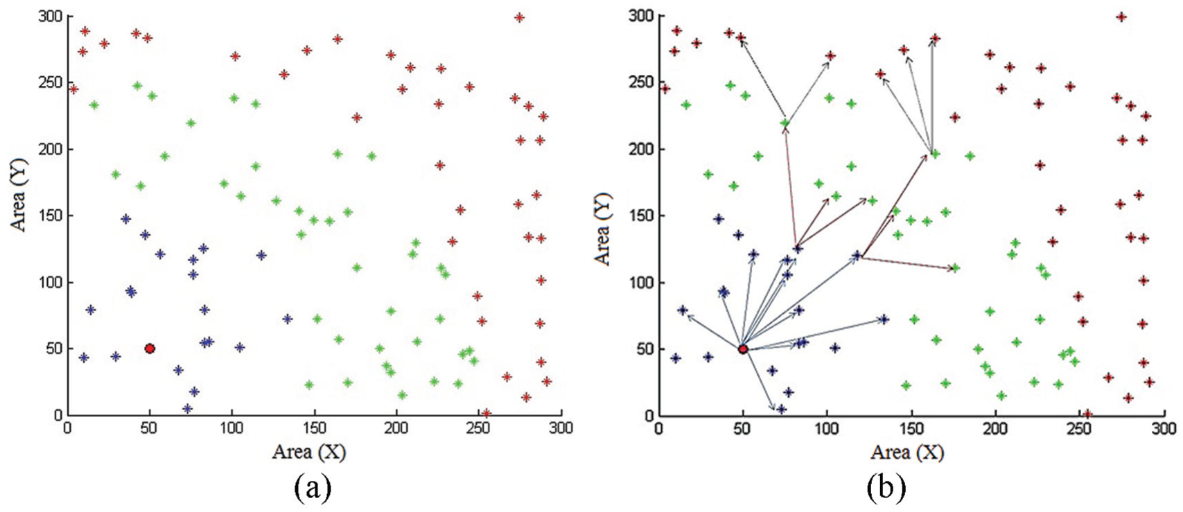
Phase 1 (a) random distributed nodes with different colors show different rings in the network and (b) initial MSG flooding from sink node into other nodes.

Finally, each node will at least broadcast one hello MSG. However, the node may broadcast more than one hello MSG if the node receives a hello MSG with Ring_ID less than its level_ID. The Ring_ID value in this message is also utilized to eliminate broadcast storm and packet loops. At the end of this phase, all nodes in the network receives the flood hello MSGs. Moreover, all nodes will have a full gateway and neighbor table.

HCRP-HD clustering phase

One of the two main methods can be adopted for clusters formation: distributed and centralized. In the distributed method, each ring with the same Ring_ID generates clusters based on LEACH clustering protocol. The optimal number of cluster heads in each ring is calculated using the same equation that has been derived in SEP routing protocol ³⁶ of all nodes in the ring.

After the completion of the selection process, each node forwards its neighbor table to its cluster head. Cluster heads compress these tables and forward them to any node in their gateway tables. The gateway nodes forward these tables to other gateway nodes in rings closer to the sink node. This process continues until nodes’ neighbors’ compressed tables reach sink node.

In the centralized method, each node sends its neighbor table to one of the nodes in its gateway table and waits for an acknowledgment (ACK). If no ACK is received, the node forwards its table to another node in its gateway table. After all neighboring tables reaches the sink node, the sink node selects the clusters and elect cluster heads. The election process is not similar to centralized LEACH since holes, edges, and transmission range are main parts of this protocol. Nodes-Rings Clustering Algorithm (NRCA) is utilized for the clustering process. NRCA will be introduced in the next section.

Moreover, the sink node generates a sequence for the nodes in each cluster to rotate the cluster head process between them without going to election process in each round. This sequence depends on nodes address “higher node address start first.” This process reduces the network overhead and energy consumption. In addition, round timers will be sent by the sink node to all nodes. These timers allow the nodes to calculate when they will act as cluster head in their cluster sequence. However, what if a node dies in the cluster that should become the cluster head next round? How the nodes in the cluster will react?

To overcome this situation, each node in the network broadcast an alive message after the expiration of a stored timer. Each node receives this alive message updates its neighboring table, gateway table and knows if the next cluster head is alive or not. If the next cluster head did not broadcast alive messages for two periods, all nodes in the cluster will delete this node from the neighboring table and from the cluster head stored sequence. In the simulation part, we attempted to simulate the centralized version of this protocol since it reduces energy consumption and messages overhead more than the distributed one.

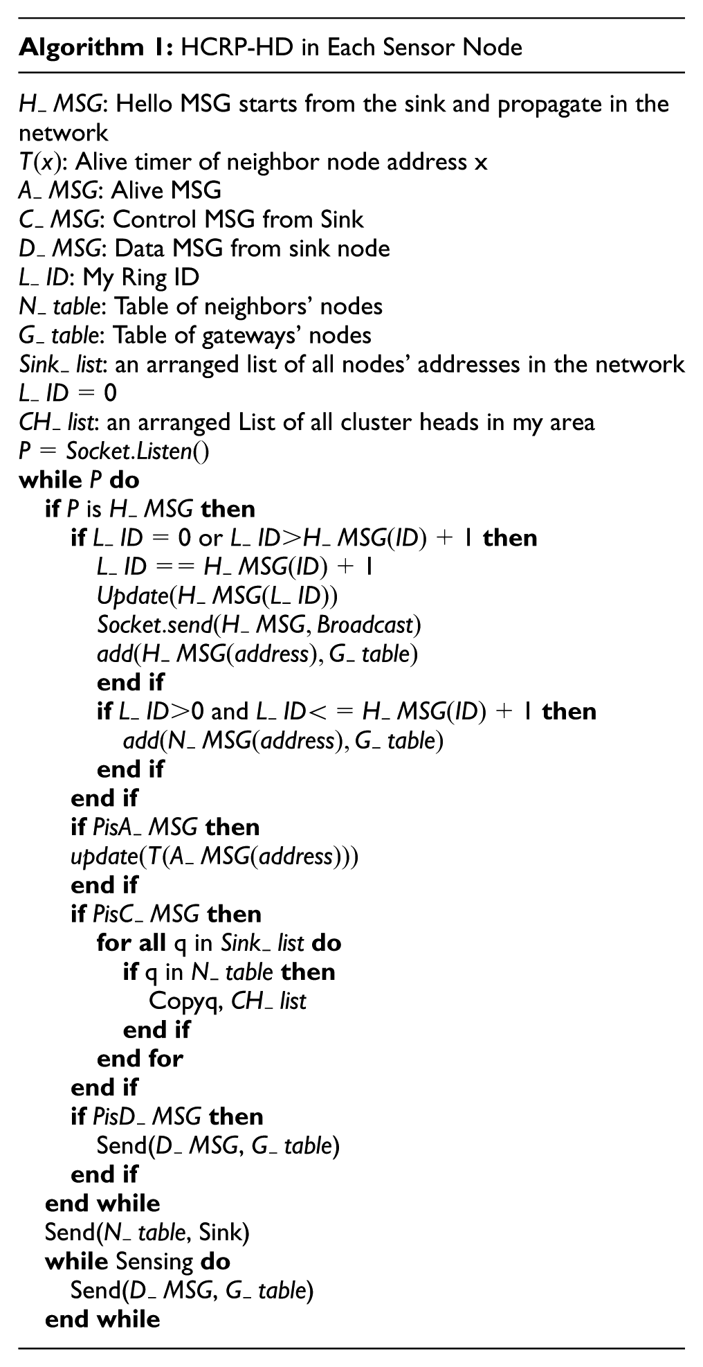
The sink node has another major role in this phase. When the sink node receives these tables, graph metrics are calculated to construct the features utilized in equations (1)–(4). Subsequently, the calculated features are fed into soft clustering to recognize outer and inner nodes. If a node is recognized as edge node, the node ID will be discarded from the cluster heads’ sequences generated by the sink node. In other words, these nodes will never be elected as cluster heads. In the following subsection, the clustering algorithm adopted in sink node will be described. Algorithm 1 shows the pseudo code of HCRP-HD runs in each node and Algorithm 2 shows the code runs in the sink node.

Algorithm 1: HCRP-HD in Each Sensor Node

$H\_\mathrm{MSG}$ : Hello MSG starts from the sink and propagate in thenetwork $T(x)$ : Alive timer of neighbor node address $\mathrm{x}$ $A\_\mathrm{MSG}$ : Alive MSG $C\_\mathrm{MSG}$ : Control MSG from Sink $D\_\mathrm{MSG}$ : Data MSG from sink node $L\_\mathrm{ID}$ : My Ring ID $N\_\mathrm{table}$ : Table of neighbors’ nodes $G\_\mathrm{table}$ : Table of gateways’ nodes $\mathrm{Sink}\_\mathrm{list}$ : an arranged list of all nodes’ addresses in the network $L\_\mathrm{ID}=0$ $\mathrm{CH}\_\mathrm{list}$ : an arranged List of all cluster heads in my area $P=\mathrm{Socket}.\mathrm{Listen}()$ while $P$ do  if $P$ is $H\_\mathrm{MSG}$ then   if $L\_\mathrm{ID}=0$ or $L\_\mathrm{ID}>H\_\mathrm{MSG}(\mathrm{ID})+1$ then     $L\_\mathrm{ID}==H\_\mathrm{MSG}(\mathrm{ID})+1$     $\mathrm{Update}(H\_\mathrm{MSG}(L\_\mathrm{ID}))$     $\mathrm{Socket}.\mathrm{send}(H\_\mathrm{MSG},\mathrm{Broadcast})$     $\mathrm{add}(H\_\mathrm{MSG}(\mathrm{address}),G\_\mathrm{table})$    end if    if $L\_\mathrm{ID}>0$ and $L\_\mathrm{ID}<=H\_\mathrm{MSG}(\mathrm{ID})+1$ then      $\mathrm{add}(N\_\mathrm{MSG}(\mathrm{address}),G\_\mathrm{table})$    end if   end if   if $\mathrm{PisA}\_\mathrm{MSG}$ then    $\mathrm{update}(T(A\_\mathrm{MSG}(\mathrm{address})))$   end if   if $\mathrm{PisC}\_\mathrm{MSG}$ then    for all q in $\mathrm{Sink}\_\mathrm{list}$ do     if q in $N\_\mathrm{table}$ then      Copyq, $\mathrm{CH}\_\mathrm{list}$     end if    end for   end if   if $\mathrm{PisD}\_\mathrm{MSG}$ then    Send( $D\_\mathrm{MSG}$ , $G\_\mathrm{table}$ )   end if  end while  Send( $N\_\mathrm{table}$ , Sink)  while Sensing do   Send( $D\_\mathrm{MSG}$ , $G\_\mathrm{table}$ )  end while

Algorithm 2. HCRP-HD in Sink Node

$H\_\mathrm{MSG}$ : Hello MSG starts from the sink and propagate in the network $T(x)$ : Alive timer of neighbor node address $\mathrm{x}$ $C\_\mathrm{MSG}$ : Control MSG $N\_\mathrm{MSG}(x)$ : Table of neighbors’ nodes of sensor node $\mathrm{x}$ $L\_\mathrm{ID}$ : My Ring ID $N\_\mathrm{table}$ : Table of all neighbors’ nodes table received $\mathrm{Sink}\_\mathrm{list}$ : an arranged list of all nodes’ addresses in the network $\mathrm{NRCA}$ : Nodes-Rings Clustering Algorithm $L\_\mathrm{ID}=0$ $\mathrm{Send}(H\_\mathrm{MSG},L\_\mathrm{ID})$ $P=\mathrm{Socket}.\mathrm{Listen}()$ While $P$ do  if $P$ is $N\_\mathrm{MSG}$ then   add( $N\_\mathrm{table}$ , $N\_\mathrm{MSG}$ )  end if   $\mathrm{Sink}\_\mathrm{list}$ = NRCA( $N\_\mathrm{table}$ )   $\mathrm{Send}(C\_\mathrm{MSG},\mathrm{Sink}\_\mathrm{list})$

Nodes-rings clustering algorithm

Nodes-rings clustering algorithm (NRCA) is a simple, hybrid “distributed-centralized,” and easy to implement clustering algorithm. It is constructed based on three main constraints. First, the number of nodes in all clusters should be approximately equal. This constraint is an important one since it was assumed in SEP protocol ³⁷ in deriving the optimal number of clusters in a network. Moreover, it was shown that heterogeneity in node numbers in clusters leads to disconnected graphs and holes in a network. ³⁶ The second constraint is to elect clusters’ heads without considering edge nodes, then finding a cluster-head sequence for all nodes to follow until the death of the network. Finally, the clustering process will not be adopted in any ring if the number of nodes in the ring is less than a threshold value. This last constraint reduces the overhead and energy consumption in the rings near the sink node. To be noted here that data required for these steps have been transmitted in the first phase of the protocol.

NRCA starts by dividing the nodes into rings according to their Ring_ID. After that, NRCA randomly selects a node with any Ring_ID from all nodes in the network to be the first cluster head in the first sequence. Subsequently, it eliminates all of its neighbors and gateways from the network. Next, another node is selected randomly as before and the process continues until no nodes remains in the network. The output of this process is the first cluster-head sequence. NRCA repeats this process again by randomly selecting a new node for the second cluster-head sequence after eliminating the nodes in the first sequence from the network. Two types of nodes are neglected in cluster heads selection process: edge nodes and nodes in rings with a number of neighbors nodes less than a threshold. In other words, these nodes are eliminated from the network before starting the first cluster-head sequence formation. The iteration process continues until all nodes in the network are participated in any cluster-head sequences. This process allows cluster heads to be distributed in the network. In other words, it is impossible to select two different cluster heads in the same range. This property is very hard to be found in distributed clustering protocols without exchanging a massive number of control overhead messages.

The threshold value that has been selected in NRCA equals the average number of neighbors for each node. To estimate this number, node density is multiplied by the maximum transmission covered area. Equation (14) shows this value. This equation can be utilized to estimate the number of nodes in each ring. However, the maximum transmission area is replaced by the size of annulus around the sink. Algorithm 3 shows the pseudo code of NRCA

$$\mathrm{Threshold}=\frac{\pi *T^2*N}{M^2}$$

(14)

Algorithm 3. NRCA

$C\_\mathrm{MSG}$ : Control MSG $N\_\mathrm{table}$ : Table of all Neighbors’ Nodes Table Received $\mathrm{Sink}\_\mathrm{list}$ : an Arranged List of all Cluster Heads in the Network $\mathrm{CH}\_\mathrm{list}(x,y)$ : Possible Cluster Heads List Nodes. Each entry hastwo properties, $\mathrm{x}$ , number of neighbors and $\mathrm{y}$ , type of the node $\mathrm{GM}\_\mathrm{table}$ : Graph metric Properties of all nodes in the network $\mathrm{TShold}$ : Average number of node’s neighbors $\mathrm{degree}(x)$ : node degree of node $\mathrm{x}$ $\mathrm{neighbors}(w)$ : neighbor nodes of node $\mathrm{w}$ $\mathrm{GM}\_\mathrm{table}$ =Calculate((Degree, PageRank, Cluster), $N\_\mathrm{table}$ ) array=Calculate(SoftCluster, $\mathrm{GM}\_\mathrm{table}$ ) for all p in $\mathrm{GM}\_\mathrm{table}$ do  if array(p)==0 and degree(p)> $\mathrm{TShold}$ then   Update( $\mathrm{CH}\_\mathrm{list}$ (degree(p), array(p)))  end if end for whilelen( $\mathrm{Sink}\_\mathrm{list}$ )<len( $\mathrm{CH}\_\mathrm{list}$ ) do  temp= $\mathrm{CH}\_\mathrm{list}$  while temp>0 do    w= $\mathrm{CH}\_\mathrm{list}(\mathrm{rand})$    add( $\mathrm{Sink}\_\mathrm{list}$ ,w)    delete(temp,w)    delete(temp, neighbors(w))   end while  end while Send( $C\_\mathrm{MSG}$ , $\mathrm{Sink}\_\mathrm{list}$ )

To show the threshold value in action, 3000 nodes have been simulated in a squared area with side length equal 500 m using Matlab. Sink node has been located in point (0,0). The maximum transmission range has been selected to be 20, 30, and 50 m. Table 3 shows a comparison of estimated numbers and numbers harvested from the simulation.

Table 3.

Threshold value simulation results.

Parameter	20 m	30 m	50 m
Estimated numberof neighbors	15.07	33.92	94.2
Average number of neighbors	15.4	33.27	86.8
Estimated number of nodes in the first annulus	3.7	8.4	23.5
The number of nodesin the first annulus	4	8	25
Number of annulusor rings	43	26	15
Number of annuluswith rings	37	21	11

One thing to be mentioned that NRCA updates the cluster-heads sequences for the network after the number of remaining nodes in the network become less than a second threshold value. The sink node receives the harvested or sensed data from all nodes in the field. When a node dies, no data will be harvested from this node. The sink node tracks these nodes to find the remaining alive nodes in the network. When a threshold value is reached, the sink node updates the cluster heads sequence for all nodes in the network.

When NRCA finishes its iterations, it forwards the sequences to all nodes in the network. Subsequently, each node marks the cluster heads in its field for each round. Moreover, it sends a joining message to one of these nodes following two main priorities. First, the node selects a cluster head if its on the node’s gateway table. Second, if no cluster head found in the gateway list of the node, the node selects the cluster head with the shortest distance.

HCRP-HD routing or data forwarding phase

The final stage of HCRP-HD is to notify edge nodes by sending a notification MSG to these nodes. When cluster heads receive notification MSG it forwards them to destinations. Other nodes in the cluster hear this MSG and mark edge nodes in their neighbor tables. In this process, edge nodes will never participate in cluster head selection. In this way they will live for longer time. However, they will participate in clusters as normal nodes.

When sensor nodes want to send data to sink node, data are forwarded to cluster head. The cluster head is responsible of gathering data from its cluster members in each ring. After that, cluster heads select a node from the gateway table and forward the gathered data to it. If the gateway table has many nodes, the cluster head will select any node not marked as an edge node. However, if the table has only edge nodes, the cluster head may select any one of these nodes. In this way, the network can scale freely in a dynamic way with any number of rings and clusters in each ring.

Experiment

To test the performance of HCRP-HD, a simulator has been developed utilizing MATLAB. Four different protocols have been programmed; two of them are used to compare energy consumption in hole and edge detection. The other two protocols are used to compare energy usage in routing process. Topological hole detection (THD) ¹⁹ and border and hole detection protocol (BDP) ⁸ have been programmed to compare holes detection and energy usage with HCRP-HD protocol. BDP has been utilized since it performed better than other protocols such as SBNs, CBNS, and DBNS ³⁸ and SDBR. ³⁹ BDP consists of three phases. In the first phase, each node collects its one hop neighbor information. In the second step, independent sets are established for nodes. These sets are used to make decisions if a node is an internal or border node as the final phase. THD on the other hand, was proposed based on isocontours. Four beacons are selected in THD. Each node, which has an equal hop count beacon, belongs to the same isocontour. Subsequently, these contours will be transformed into connected components and holes will be detected. This protocol has been selected since it is easy to implement.

The third protocol, which has been written is LEACH-T Al. ⁴⁰ This protocol is one of the LEACH family members that adopt the hieratical routing in the network. It has been programmed to compare energy usage of the routing process through the network without edge and hole boundary nodes. LEACH-T is a LEACH-based protocol that converts the network into number of clusters. Each cluster contains a head node that has been elected to collect data from other nodes. The protocol routes data from head nodes to sink node in a direct connection if the distance between the head and the sink is less than a threshold. However, if the distance is larger, an intermediate head from another cluster is responsible of delivering the data. Another threshold value is used to route data from the intermediate head to another head more near to the sink node if the distance crossed the second threshold. This protocol has been used since it tolerates long transmission distances with multilayered routing of data.

The final utilized protocol is the SEP protocol. Unlike the first three protocols, this protocol adopts energy heterogeneous model of the nodes in the WSN field. This protocol is also a member of the LEACH family, which adopts the same cluster formation process. It has been used in this work to show how the heterogeneity property of the nodes is not important than edge nodes and disconnected network graphs.

A network consists of 3500 nodes distributed randomly in an area of 500 × 500 m. Two holes have been generated in the network as squares with 100 × 100 m size. This model has been utilized in Nguyen and Bai. ¹¹ A sink node has been added to the network in location (0, 0). An energy of 0.5 J has been added into each node in the network. A packet size of 2000 byte is transmitted in each round in the clustered protocol. Table 4 summarizes the environment configuration parameters.

Table 4.

Environment configuration variables.

Variable	Value
Number of nodes	3500
Size of network	500 × 500
Packet size	2000 bytes
Sink node’s location	(0,0)
Initial start-up energy	0.5 J
Number of holes	2

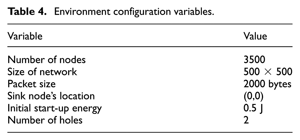
Figure 3 shows the network after distributing the nodes. Two simulation applications have been used; MATLAB and Gephi. ⁴¹ Gephi is a graph analyzing software that is capable of extracting graph properties and filter their results. In this work, Gephi has been leveraged for feature selection process. In the following sections, we will explain the conducted experiments and results of feature selection, soft clustering, and HCRP routing.

Figure 3.

WSN environment with holes (a) nodes distribution in MATLAB and (b) network view in Gephi.

Feature selection

To select features, IG is used. However, to show the impact of graph metrics in detecting holes and edges’ nodes, Gephi has been used. Gephi, as mentioned, is open source software that has been developed to study different type of graphs. Gephi has the ability to filter graphs according to different graph metrics. It also has s presentation view of graphs with different drawing algorithms. For example, Figure 3(b) has been drawn using force2 algorithm. We used Gephi to calculate five graph metrics, node degree, local cluster coefficient, betweenness, closeness, and PageRank. Subsequently, for each metric, we have filtered nodes according to the calculated values. We utilized this graphical method to present the impact of graph metrics in holes and edges’ detection. Figure 4 shows the output of Gephi. We have filtered nodes according to 100%, 75%, 50%, and 10% value of each parameter or metric.

Figure 4.

Graph metrics filtering according to (a) closeness values, (b) local clustering coefficient values, (c) betweenness value of each node, (d) PageRank value, and (e) node degree.

We can observe from Figure 4 that closeness centrality graph metric can detect edges’ nodes. However, holes’ nodes cannot be detected. We can observe this from the last network in Figure 4(a). We also can observe that corner nodes can be recognized easily with this metric. Local clustering coefficient can detect edges and holes. However, we can observe the missing properties of holes in the last network in Figure 4(b). In Figure 4(c), Betweenness centrality is shown. As in closeness, betweenness is good in detecting network edges’ nodes. However, the characteristics of holes are missing in the last network in Figure 4(c). In Figure 4(d), PageRank algorithm has been used. We can observe that its accuracy is better than local clustering coefficient. Finally, in Figure 4(e), node degree is used. The output in the last network detects all edge and inner nodes. However, it requires more filtration.

To find the impact of each one of the graph metrics on the detection process of nodes mathematically, IG has been leveraged. Each node has been classified as inner or outer node. Outer nodes are the edge nodes beside holes or at network borders and inner nodes are the rest. Equations (5) and (6) have been used to calculate IG. Table 5 shows the output. We can observe that node degree, PageRank, and local cluster coefficient have the highest impact in this clustering process. These three metrics have been selected as features in the clustering process.

Table 5.

IG values for different features.

Feature	Value
Node degree	0.89
PageRank	0.88
Local cluster coefficient	0.82
Betweenness	0.41
Closeness	0.32

Soft clustering (EM)

In this section, we utilized the graph metrics PageRank, local cluster coefficient and nodes degree in clustering nodes into inner and outer nodes. MGD has been used with ML. The clustering process output has three different clusters: inner “not beside borders or holes,” outer “beside holes or at the edge,” and unclassified nodes. The unclassified nodes can belong to any one of these clusters. When the threshold value increases, these nodes finds a cluster and participates in one cluster. Figure 5 shows the clusters in this network. Three colors have been used: red, blue, and black. We can observe that unclassified (black) nodes are located in areas with less dense nodes than other locations. These nodes are not edge or hole nodes. The low density of the nodes in their areas tricks the clustering algorithm. However, the algorithm does not classify these nodes and keeps this process to the user to classify them in any cluster. Figure 5 compares HCRP-HC clustering with BDP and THD protocols. However, it is very hard to compare these models pictorially. We compared the accuracy of these algorithms in Table 6. Missed nodes in this table are the edge or hole nodes that have not been detected and incorrect nodes are the inner nodes that have been classified as edge nodes. We can observe that HCRP-HD did not classify any outer nodes as inner nodes.

Figure 5.

Comparison of edge and hole detection (red: edges nodes, blue: internal nodes), (a) HCRP-HD protocol (black nodes are not classified as holes or internal nodes), (b) BDP protocol and (c) THD protocol.

Table 6.

Accuracy comparison.

Protocolname	Missed nodes (%)	Incorrectnodes (%)
BDP	1	3
THD	2	12
Proposed	0	1

Finally, we have generated different holes’ shapes to show the accuracy of the clustering technique. Figure 6(a) shows an E-shaped hole. Figure 6(b) shows a random shaped hole. We can observe how the clustering adapts to different shapes. We can observe in the random hole network that the clustering process has too many unclassified nodes “black colors” since the density of nodes in many areas in this network is lower than other configurations. We also can observe how the “E” hole has been detected in an accurate way.

Figure 6.

Different holes’ shapes, (a) E-shaped hole, and (b) random shaped hole.

HCRP-HD cluster formation

To study power consumption of HCRP-HD, the clustering formation process is studied. HCRP-HD divides the network into a number of rings. In each ring, a number of clusters are constructed. However, if the number of nodes in the ring is under a threshold value, no cluster formation occurs. Figure 7 shows the relationship between ring formation and the transmission range of all nodes. We can observe that with lower transmission range the number of constructed rings increased. This will increase the number of hops in the path between the source and destination. However, the energy consumption will not increase compared with LEACH-T as shown in the last section. Figure 7 has been generated with averaging 30 iterations of node distribution for each transmission range.

Figure 7.

Relationship between transmission range and number of rings in the network.

To study the impact of edge and hole boundary nodes elimination from the routing path to the sink node, HCRP-HD protocol has been utilized with and without the elimination process of outer nodes from the routing path. 30 iterations have been recoded. The average routing path has been calculated for each node in the network. Subsequently, these paths have been averaged over 30 iterations. The final paths have been added and averaged over the number of nodes in the network. Table 7 shows a comparison between path length in both cases. We can observe that the average length of paths with and without the elimination process are approximately the same since the number of nodes in the network is large. This shows that the elimination process of outer nodes from the routing process will not reduce the network performance, and it will not increase the delay. However, it will keep the network connected for longer time.

Table 7.

Comparison between path lengths of HCRP-HD with and without hole and edge nodes elimination.

Protocol	Path length (hops)
HCRP-HD with elimination	5.4 hops
HCRP-HD without elimination	5.3 hops

HCRP-HD energy consumption

This section is divided into two subsections. In the first part, computation energy consumption by the HCRP-HD protocol is estimated. In the second part, energy consumption in hole detection and data forwarding will be shown.

Computational energy consumption

To estimate energy consumption due to computational complexity of the protocol, we programmed the protocol using C language and implemented it in ATmega328A microcontroller with Xbee module for data transmission. Moreover, we programmed the LEACH clustering protocol for the same platform to compare computational energy consumption of HCRP-HD and LEACH. ATmega328 has been selected with low oscillation frequency of 8 MHz, 3.3 v, and 3 mA. The CPI of this controller is approximately 1. We programmed the clustering process, a semi-TDMA selection, joining and data harvesting processes. However, the protocols have not been experimented in massive platform since our objective here is to estimate the number of instructions in each protocol.

After compiling the C code for each controller, the output HEX file has been used to count the number of instructions, the format of this file follows Intel HEX file format with eight 16-bit instructions in each line. Moreover we counted the number of instructions that will be repeated each round in each protocol. For HCRP-HD, the number of instructions was 3208 instruction with 290 repeatable instructions in each round. However, for LEACH, the number of instructions was approximately 8320 with approximately 1200 repeatable instructions each round. This means that HCRP-HD consumes 3900 nJ in the initialization phase and for each round 358 nJ. On the other hand, LEACH requires 0.01 mJ for initialization and about 1.48  $\mu$ J each round. It is worth mentioning that the power consumption of HCRP-HD in the clustering process has not been estimated since the sink node is responsible of this part.

It is worth mentioning that the number of instructions should be counted only in run time to count the number of assembly instructions inside loops. However, in our situation, it was easy to count them before run time. In cluster WSNs, nodes are categorized as normal and cluster heads. Cluster heads codes have loops with “while” conditions that depend on the number of nodes connected to them. The number of executed instruction in these nodes can only be counted at runtime. We did not estimate power consumption of these nodes. What we have done is counting the number of instructions in normal nodes.

In the proposed protocol, these nodes sense the environment and forward the data. When the hex file has been read, we searched for the “conditional Jump” instruction to count the number of repeated instruction. All the conditional Jump instructions have the same conditions that do not depend on any run time variables. However, in LEACH an issue has been found.

For LEACH, in each round the clustering phase “voting or cluster head selection process” occurs. Five percentage of the nodes is selected as cluster heads in each round. Moreover, any node becomes a cluster head every 20 rounds ones. These numbers are real assumption from the LEACH implementation. In this phase, each node calculates the probability variable that shows if a node will become a cluster head or not. If the node is not a cluster head, the nodes will wait to receive messages from all new cluster heads to select one of them. The selection process is a loop over all the messages to find the nearest cluster head using the highest RSSI value. This loop depends on a run time variable, which is the number of cluster heads in the network. We have counted the cluster head selection instructions only one time and neglected this loop since the number of cluster heads will be limited and this loop consisted of only one instruction.

Finally, it is worth mentioning that the number of instructions in each protocol can be optimized or reduced if other programmer develop these protocols. Moreover, the physical implementations of these protocols are impossible with the adopted energy transmission model. These facts motivated us to neglect the computational energy consumption in the next sections.

Hole detection energy consumption

Figure 8 shows the energy consumption of THD, BDP, and HCRP-HD in the hole detection process. 30 runs have been averaged to produce this figure since nodes are distributed randomly in each run. We can observe that energy usage is massive in these protocols compared with HCRP-HD since the detection process is a centralized process done by the sink node. One thing to be mentioned that energy usage in the computational process have been neglected. If equation (13) is utilized, energy usage of THD and BDP will be massive. The massive consumption of energy reduces network life time, and it will increase the number of produced holes in the network. Moreover, these protocols have been proposed for holes detection process only. HCRP-HD has been constructed with the detection process and the routing procedure to leverage the detection results.

Figure 8.

Energy consumption of hole detection process.

Figure 9 shows the number of overhead messages utilized in the detection process. This number depends on the number of nodes in the network. The overhead messages are divided into two main messages, holes detection and cluster formation messages. The second type of messages have been neglected in HCRP-HD protocol since these messages are not implemented in THD or BDP. We also can observe that the number of overhead control messages in HCRP-HD is small compared with THD and BDP. This prolongs network life time in one hand and reduces traffic congestion on the other hand.

Figure 9.

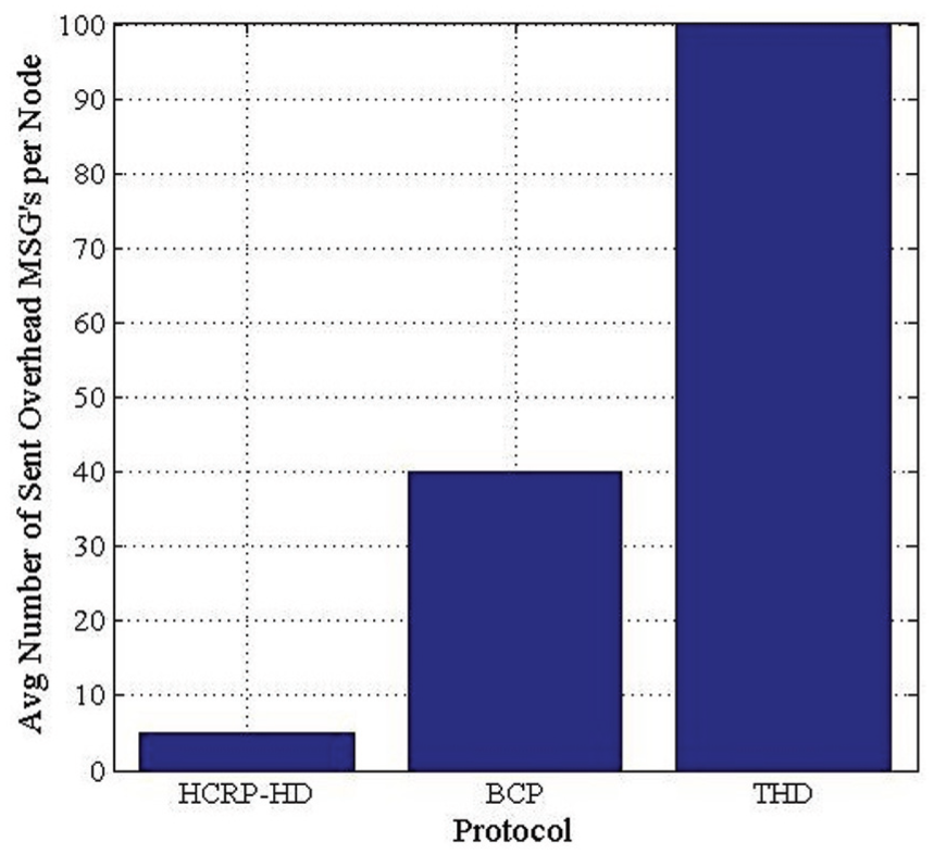
Number of overhead messages utilized in the detection process.

Routing process energy consumption

Finally, we compared HCRP-HD routing process with LEACH-T protocol and SEP. Figure 10 shows a comparison of network life time of the three protocols. We can observe from the CDF that approximately 50% of the nodes lived more than 1600 rounds, which is a massive number compared with LEACH-T and SEP. On the other hand, we can observe that LEATH-T extended the network life time more than SEP since it adapts a hierarchical routing with the clustering unlike SEP that utilizes clustering with linear routing of the data from cluster heads to sink node with only one hop. This module is impossible in real situation. Finally, We can observe that the network life time was prolonged by 10% or more compared with LEACH-T.

Figure 10.

Average energy consumption in each protocol.

In Figure 11(a) and (b), only LEACH-T and the proposed protocol has been compared since in SEP no disconnected graphs or isolated nodes may occur according to the assumption they adopted in the power model, which note that any node can reach the sink node at any distance. Figure 11 shows the number of disconnected graphs generated in both protocol through the simulation process.

Figure 11.

LEACH-T comparison: (a) number of disconnected graphs and (b) number of isolated nodes.

We can observe that LEACH-T generated many isolated clusters that data cannot be harvested from them. These clusters collect data that cannot be passed to the sink node. Finally, Figure 11 shows the number of isolated nodes in the simulation process in HCRP-HD and LEACH-T. We can observe that far nodes become isolated in HCRP-HD after 60% of nodes in the network die. This percentage can be enhanced with the enhancement of the clustering process in each ring.

Conclusion

In this work, a new hybrid clustering routing protocol in WSN is proposed, namely, HCRP-HD. This protocol aims to prolong network life time through detecting holes and edges nodes. The protocol consists of two main layers: hole detection and packet routing. The detection process attempts to generate a connected graph without any isolated nodes or clusters that have no path to the sink node. EM soft-clustering technique has been utilized with three graph metrics: PageRank, node degree, and local cluster coefficient. In the routing process, HCRP-HD converts the network into a number of rings to overcome energy consumption of different direct transmissions between cluster heads and the sink node. We compared HCRP-HD with three different protocols; BDP, THD, and LEACH-T. Our result shows that holes detection accuracy reached 98%. Moreover, network life time has prolonged 10%. Finally, HCRP-HD eliminated the disconnectivity in the network for more than 80% of network life time. In the future, we will attempt to deploy this protocol in real nodes.