Sage Journals: Discover world-class research

Abstract

In the last decades, studies on travel mode detection from location data have been increasing exponentially. However, these studies have struggled with three limitations: data collection-, feature selection-, and classification approach–related issues. Thus, we propose a novel framework to collect trajectory data and infer travel modes by making a great deal of effort. First, we conduct a travel survey with smartphones in Shanghai City, China. Furthermore, we use a prompted recall survey with surveyor intervention by telephones. In the survey, the surveyor asks respondents to validate the travel information automatically detected from trajectory data. Second, we use well-known sequential forward selection procedures to select the most reasonable combination of features. This set of features is expected to help achieve high classification accuracy with few features. Third, as a machine learning approach incorporating high resistance to noise in features, a continuous hidden Markov model is used to classify segments in dataset 1 that comprises Global Positioning System data alone. Consequently, 94.37% of segments are flagged correctly for the training dataset, while 93.47% are detected properly for the test dataset by making a comparison between detected travel modes and travel modes validated during the prompted recall survey. A higher accuracy (95.28%) is achieved in the test dataset on dataset 2 that consists of Global Positioning System, accelerometer, Global System for Mobile communication, and Wi-Fi data. The promising results obtained with this method provide a new perspective in understanding travel mode detection and other related issues in Global Positioning System travel surveys, including trip purpose detection.

Keywords

Travel mode travel survey continuous hidden Markov model classification combination of features

Introduction

Traffic congestion in cities has increasingly spread in terms of temporal and spatial ranges. Transportation infrastructure investment was significantly increased to ease congestions by increasing the supply of transportation. However, this strategy did not evidently improve the performance of transportation networks as we expected because increased traffic demand was stimulated using newly built traffic facilities.¹ In the past couple of decades, transportation planners have, therefore, attempted to regulate traffic demand by establishing and implementing feasible demand management policies that depend on daily travel patterns of residents.^2,3 Household Travel Surveys (HTSs) and Personal Travel Surveys (PTS) are generally used to collect explicit travel attributes, including travel destinations, travel timing, travel modes, trip purposes, and sociodemographic characteristics.⁴ The data collected are usually used to derive daily travel patterns and policies for transportation demand management.

Traditional HTSs/PTSs are generally executed through retrospective surveys or diary surveys, in which respondents either report their travel information in face-to-face/telephone interviews or record their travel information on paper-based/Internet-based questionnaires. Therefore, respondents need to remember start and end times, origination and destination locations, travel modes, and trip purposes and undertake a heavy burden. Moreover, respondents tend to approximate travel timing as the adjacent 5 min, 10 min, and even half-hour, as well as underreport trips with a short distance or duration. These issues encountered by traditional HTSs/PTSs necessitate the development of a new mode of travel surveys.⁵ As Global Positioning System (GPS) positioning devices with high accuracy have become technically mature and economically acceptable, researchers gradually conduct HTSs/PTSs with GPS as viable alternatives to conventional surveys. As a new technology, GPS has been applied in travel surveys since the later part of the 1990s. The first travel survey with GPS was implemented by the Federal Highway Administration in 1996 to track vehicles and to record vehicle trajectories of respondents.⁶ Thereafter, travel surveys with GPS have been increasingly applied in a large number of countries, including Canada, Denmark, Israel, the Netherlands, Sweden, Australia, United States, United Kingdom, Austria, France, Japan, and Switzerland.⁷

Travel information, including travel modes and trip purposes, cannot be derived directly from travel surveys.^8–10 This study aims to derive travel modes automatically from GPS trajectory data. Travel mode detection is a classification issue, which is an example of pattern recognition in computer science. In this issue, the problem of identifying the set of travel modes to which a new observation belongs is based on a training dataset of samples (or observations) whose travel modes are known.^11,12 Travel mode detection is also a multiclass classification problem, which often requires the combined use of multiple binary classifiers because many classification methods are developed particularly for binary classification. Travel modes are generally detected with rule-based or machine learning approaches. Rule-based approaches are easy to understand and produce a good classification result in some situations. However, machine learning approaches have an advantage over rule-based approaches because of the preferable generalization ability and potentially flexible and robust superiority of the former in handling issues in multiple contexts.¹³ Travel mode detection with machine learning approaches consists of three steps: data collection (involving the device used to record GPS data, the method of validating travel information, and sample size), feature selection for classification (involving the selection of the best feature set), and classification approaches (involving details of classification approaches used). Accordingly, the limitations on these efforts can be classified into three categories: data collection-, feature selection-, and classification approach–related issues.

Issues associated with data collection in HTSs/PTSs with GPS compromise the device for recording trajectories and methods for validating travel information. Most existing studies used dedicated GPS devices in collecting GPS data. However, travel surveys with dedicated GPS devices incorporate the following limitations: (1) the high cost for purchasing devices is undertaken, (2) incomplete data are usually collected because respondents often forget to take along the devices with them (3) devices must be distributed/recovered as long as a respondent participates in/exits this survey, and (4) sample size is limited by the number of dedicated GPS devices available.¹⁴ Another issue on data collection is the validation of travel information, which is crucial in developing automated algorithms to extract travel information from the raw GPS positioning data streams. Prompted recall (PR) surveys have emerged as effective surveys to improve the accuracy of the travel information collected. In the PR survey, respondents usually receive a map with travel trajectories of a whole day based on geographical information system (GIS) sources. This map can be used to prompt respondents to recall detailed travel information. A recent PR survey by Cottrill et al.¹⁵ allowed respondents to modify the detected travel information (e.g. inserting/deleting trips and changing travel modes/trip purposes) online to derive the actual travel information. However, respondents may not easily master the operation to modify the derived travel information even when detailed explanations and materials are provided. For example, respondents could not easily understand the difference between a trip and an activity. Therefore, self-administered travel surveys may result in because no surveyors prompt respondents to recall detailed information.¹⁶

Feature selection is one of the most crucial issues related to travel mode detection from GPS data. The central premise to use a feature selection technique is that features extracted from the input data are irrelevant or redundant; thus, certain features can be removed without incurring considerable loss of information.¹⁷ The features used in existing studies on travel mode detection from GPS trajectory data generally include speed, maximum speed, 95th percentile speed, median speed, and acceleration. These speed-related features may have a strong correlation with one another. However, most studies did not discuss feature selection techniques in detail and explore the method to choose an appropriate feature selection technique thoroughly.

The machine learning approach determines the classification accuracy of travel mode detection to a large extent.¹⁸ From an empirical perspective, a variety of machine learning approaches are used in existing literature, including decision trees,¹⁹ Bayesian networks (BNs),²⁰ naive Bayesian classifier,²¹ fuzzy logic,²² hierarchical conditional random fields,²³ discriminant function analysis,²⁴ and support vector machines (SVMs).²⁵ A few studies detected travel modes based on single-mode trip legs (hereafter referred to as “segments”) or split trajectories according to a given length or duration to maximize information stored in the trajectories with small time windows, such as 1 or 2 min. A segment is a portion of travel on exactly one transportation mode. In order to divide a trip into segments, mode change points must be identified. They are the first and last points of a gap or of a walk segment that is longer than 60 s. Mode change points divide a trip into multiple segments. Parlak et al.²⁶ imputed travel modes based on GPS trajectory data with “instant mode determination” and “trip mode determination” steps. In the first step, segments were derived with a threshold of 10 min, and each segment was matched with a travel mode using the random forest classifier. In the second step, a discrete hidden Markov model (DHMM) was trained for each class with actual travel modes as the hidden state set and the estimated travel modes as the observation symbol set. Travel modes were detected at the trip level. Similarly, a DHMM was used to detect travel modes.²⁷ As a classifier to cope with sequence data, a hidden Markov model (HMM) is an appropriate approach for detecting travel modes. The most significant advantage of an HMM versus aforementioned classifiers is the direct application of the former to the continuous data stream, which enables pattern recognition based on features with small granularity.²⁸ Travel mode detection with the aforementioned classifiers consists of the feature extraction and the class determination. The feature extraction transforms raw trajectory (including a number of GPS points) into a few features according to predefined formula, and the extracted features are fed into classifiers to determine travel modes. For example, the instantaneous speed of all GPS points is averaged into the feature named “average speed.” In this case, the information loss is inevitable due to the dimension reduction. In comparison, HMM takes full advantage of the information stored in the trajectory by analyzing the GPS points directly. The main difference between a DHMM and a continuous HMM (CHMM) is the treatment of observation. Specifically, observation probabilities are computed from a look-up table in a DHMM and are calculated based on the continuous feature vectors in a CHMM. A DHMM generally takes less time than a CHMM, but the former may incorporate lower prediction ability than the latter.²⁹ In the current study, travel modes are detected after the data collection process rather than simultaneously with this process. Therefore, more emphasis should be placed on prediction ability than computation time.³⁰ On the contrary, a DHMM is a powerful classifier that performs well on classification problems for a large training dataset with the temporal dimension, particularly tens of thousands of training samples for each class in a classification issue, whereas a CHMM is an appropriate classifier when a training dataset is small. Although we have recruited hundreds of respondents to take part in the smartphone-based travel survey in this study, the sample size might be too small to enable the sufficiently powerful prediction capability of a DHMM. In case studies, the application of a CHMM was recommended because of its prediction accuracy in most of the existing works comparing a CHMM with a DHMM; these works include studies on speech recognition.²⁹ An exception is an effort on handwriting recognition by Rigoll et al.³¹ Although the authors attributed this result to an unusually high number of states per HMM, they believed that the result is generally not the case. In the current study, CHMM is used based on the theoretical analysis and results from case studies.

Thus, we try to understand and improve on the travel mode detection in the current study. First, we conduct a travel survey based on smartphones in Shanghai City, China. In this survey, we use a PTS with a surveyor-intervened PR survey with telephones, in which the surveyor reminds the respondents to check travel information imputed from GPS trajectory data. Second, we use well-known sequential forward selection (SFS) procedures to extract the most reasonable set of features. This set of features is expected to help achieve high classification accuracy with few features. Third, as a machine learning approach incorporating high resistance to the noise in features,³² a CHMM is used to classify GPS data into one of the five travel modes (i.e. walk, bicycle, e-bicycle, bus, and car).

The remainder of the article is arranged as follows. The procedures of the smartphone-based travel survey with a surveyor-intervened PR technique are reported under the “Data collection and description” section, whereas the distribution of features and the details associated with SFS are presented under the “Feature extraction and selection” se1ction. The theoretical foundation of CHMM and its application in detecting travel modes are elaborated under the “Travel mode detection with CHMMs” section. Finally, conclusions and future directions are presented under the “Discussion and conclusion” section.

Data collection and description

Data collection comprises respondent instruction and data validation. Each respondent is assigned a dedicated user ID generated automatically after installing a designated application (iOS and Android versions are available so far). The respondents are also asked to start the positioning application and then upload the positioning data each day during the period of the survey. The application can record altitude, longitude, latitude, time, instantaneous speed, and accuracy with 1 Hz frequency for both Android and iOS versions. In the absence of a GPS location service, both Android and iOS versions record the estimated location according to Global System for Mobile communication (GSM)/Wi-Fi networks. However, the iOS version does not share the source of location data with applications and thus, we cannot determine whether the location data are from GPS or GSM/Wi-Fi.³³ As a result, we can only delete possible GSM/Wi-Fi location data for the iOS version based on the accuracy measure, and the remaining location data are regarded as GPS data.²⁶ The accelerometer data are collected by the application for Android operating system with 1 Hz frequency, which is expected to improve the accuracy for travel and activity recognition.³⁴ Data validation is performed in such a way that surveyors call respondents to remind them to validate the travel information derived from the trajectory data. Figure 1 shows the flowchart of the survey. In this survey, PTSs are undertaken instead of HTSs because other household members may not use a smartphone when a certain member is recruited.

Figure 1.

The flowchart of the smartphone-based travel survey.

Respondent instruction

Survey instructions, including survey purposes, operation manual of the application, and other issues, are also vital to the survey in this study. Respondents can be encouraged to participate in this survey, start the application in time, and validate the derived travel information by elaborating survey purposes. Respondents can be encouraged to participate in this survey, start the application in time, and validate the derived travel information by elaborating survey purposes. Other issues include the application and embedded GPS units should keep running between the beginning of the first trip and the ending of the last trip, and the explicit attributes of all trips should be under attention during the whole survey period. All these requirements are designed to enable complete positioning data streams and to enable respondents to maintain a clear memory of the actual travel attributes. In addition, it is crucial for this survey to handle privacy issues reasonably. To decrease the worries of respondents about privacy issues, we explicitly explain the measures that are taken to overcome the privacy issues. On the one hand, respondents can examine the authorities achieved by the app and check whether the app collects sensible information; on the other hand, respondents can receive a commitment letter explaining that the application of the collected data is confined to scientific research alone and that the data collected are anonymous and kept secret.

Data validation

PR surveys are widely recognized as effective methods to capture the actual travel information.³⁵ Most of the existing studies used a self-reported PR survey.³⁶ In this PR survey, respondents are provided with maps with trips and stops detected automatically from the GPS data they recorded. They are also required to correct detected trips and trip-related attributes (including travel modes) when necessary. However, the respondents may have a different understanding of the notion of “trip” and may report their trips at different accuracies, in which the data quality of travel information depends highly on the respondents in a self-reported survey. Therefore, a PR survey joined by surveyors with telephones is used to derive the most complete and most accurate travel information possible. The respondents can access their travel trajectory using an account provided by surveyors at the beginning of the survey. Most respondents are interested in browsing their travel trajectories, which can also help to collect complete positioning data and actual travel information. On the contrary, the surveyors can prompt respondents to recall related information with telephones according to the travel information derived from raw positioning data. The surveyors also send reminders via e-mail or text message to prompt the respondents to start the positioning application in time, thereby improving the possibility of collecting complete GPS data streams. In the process of data validation, the surveyors may need to conduct various types of operations, such as adding, deleting, and modifying initial records derived from raw trajectories. These operations are similar to those in Pereira et al.³⁷

Data description

A total of 352 respondents took part in this survey, but 31 of them quit because of device failure or an unexpectedly long business trip. In terms of the types of smartphones used, 187 completed the survey using Android-based smartphones and the remaining 134 used iOS-based smartphones (iPhones). This survey eventually collected travel information of 2409 persons/day from 321 respondents from October 2013 to June 2015. The survey lasts for a long duration because the seasons for data collection affect the travel mode detection. Specifically, the features for travel mode detection have different distributions for different seasons and the detection accuracy for datasets from different seasons also varies.³⁸ More specifically, 246 completed this survey of 7 days, while the others range from 8 to 12 days. A total of 85 were randomly chosen to answer several questions on the survey after they completed the survey. One of these questions was whether the application caused battery drainage. The 85 respondents comprised 56 Android users and 29 iOS users. A total of 10 Android users (17.86%) and 7 iOS users (24.24%) reported battery drainage caused by the application. Figure 3 shows that the mean and standard error of GPS points were 8.39 and 3.48 m, respectively. An average duration for each respondent participating in this survey reached 7.5 days such that the data could be used to analyze multi-day travel behavior. The percentage of complete positioning data was 76.71%; that is, 1848 persons/day of data remained complete. Travel modes were first detected on dataset 1, comprising only GPS data from both systems, to develop a compatible method on both Android and iOS systems. Travel modes detected on dataset 2, which consisted of GPS, GSM/Wi-Fi, and accelerometer data from Android system, were used to evaluate the usability of GSM/Wi-Fi and accelerometer. All statements are based on dataset 1 until section “Classification results on dataset 2.”

The walk, bicycle, e-bicycle, car, bus, and other modes (not belonging to any previous travel mode) were reported in the travel survey, and the previous five travel modes are detected in the current study. All GPS data were split into segments in accordance with the validated trips. In general, a trip may incorporate several segments. For example, an individual walks to a bus stop, takes a bus, and then walks to a shop. This trip includes two walk segments and one bus segment. A validated mode was assigned to each segment. A total of 6982 segments were extracted according to the validated travel modes. Figure 2 shows that walk mode has the highest proportion, which may be due to that walk modes are usually used during intermodal transfers. For example, a traveler may walk to a bus station after getting off a subway line if he or she needs to transfer from the subway mode to the bus mode. A significant difference in percentages was not observed among the other travel modes. Remarkably, e-bicycle segments, which are often considered to be motorized, has a substantial proportion because of a great convenience and a low purchase/use cost of e-bicycles.

Figure 2.

The number of segments with five travel modes.

Feature extraction and selection

Features regarded as inputs of a classifier should have a strong influence on the classification accuracy of travel modes. These features can be determined with the following steps: feature extraction and feature selection. Feature selection aims to derive relevant features on travel mode detection from GPS data, whereas feature selection attempts to remove redundant features without incurring considerable loss of information and to retain other features for further analysis.

Feature extraction

A feature set that is highly relevant to travel mode detection may help to improve the classification performance. Average speed, average absolute acceleration, traveled distance, and 95th percentile speed are usually used to impute travel modes. However, it may be difficult to make a distinction between car and bus modes as well as between bicycle and e-bicycle modes if only the speed-related features are applied.³⁹ In general, the application of a bus network layer may increase the classification accuracy of car and bus modes.⁴⁰ Nevertheless, bus networks are updated monthly and even daily in mega cities. A timely update is required to detect bus segments effectively. In this case, it may be rather costly to maintain an up-to-date bus network, which motivates us to extract a novel feature we refer to as “low-speed point rate”; that is, the rate of GPS points with the speed of less than 1 m/s. This feature is expected to reflect the fundamental characteristics of periodical stops of bus segments. Four different critical speeds, namely, 0.5, 1.0, 1.5, and 2.0 m/s, are investigated to extract this feature. As a result, 1 m/s is used because it makes the most obvious distinction between bus and car modes. In addition, the uncertainty of speed-related features may potentially decrease the classification accuracy.⁴¹ For instance, a bicycle segment with a relatively high speed may be mistakenly identified as an e-bicycle segment. However, an e-bicycle does not usually change the riding direction unless necessary. By contrast, a traveler riding a bicycle may stop or overtake others more casually. Thus, we develop another novel feature called “heading change rate,” which is denoted as the average heading change between all pairs of two consecutive points. In summary, two novel features, besides the four frequently used ones, are used to differentiate five travel modes.

Each segment should be split into a specified number of subsegments with equal duration to impute travel modes from GPS trajectory data with a CHMM. A CHMM assumes that observations are independent because of hidden states. If the specified number is large, then each subsegment can last for only a few seconds, and the assumption of independence may be violated. If the specified number is small, then the classification accuracy of the CHMM may be low. Therefore, each segment is split into 10 equal subsegments to enable a reasonable time window for each subsegment.²⁷ Features are extracted from each subsegment (Figure 3).

Figure 3.

Features at a subsegment level.

The abilities of different features to distinguish travel modes vary. Figure 4 displays the distribution of 69,820 subsegments with respect to six features. The probability density functions of 95th percentile speed and the average speed are similar in the sense that the latter appears to be twice longer than the former on the horizontal axis (as shown in Figure 4(a) and (b)), except that the latter appears to be more representative than the former. This similarity indicates that both features are stable and different from the maximum speed, which tends to fluctuate significantly due to positioning errors. Both features divide five modes into three classes, that is, walk as a class; e-bicycle and bicycle as a class; and car and bus as a class. Average absolute acceleration is another valuable feature applied to impute travel modes. In terms of average absolute acceleration, the car, bus, and e-bicycle segments have similar distributions with each other and are distributed differently from other modes (as shown in Figure 4(c)). Regarding traveled distance, there exists a high affinity between car and bus modes, and a relatively low similarity exists between these two modes and the other three modes (as shown in Figure 4(d)). Just as we have expected, low-speed point rate may make an obvious distinction between walk and other modes as well as between bus and car modes (as shown in Figure 4(e)). Furthermore, motorized and non-motorized modes seem to incorporate two different patterns in terms of heading change rate (as shown in Figure 4(f)).

Figure 4.

Distribution of extracted features: (a) average speed, (b) 95th percentile speed, (c) average absolute acceleration, (d) traveled distance, (e) low-speed point rate, and (f) the average heading change.

Feature selection

Feature selection plays a key role in decreasing the complexity and improving the classification accuracy of a classifier. Inspired by fusion approach,^42,43 a feature selection algorithm is the combination of a search technique to construct new feature sets and an evaluation measure that rates feature sets. Most previous studies detected travel modes according to predefined features, some of which may be unnecessary in terms of the classification accuracy. Therefore, we use the well-known SFS procedures to choose the most powerful features. The SFS is used to maximize the overall classification accuracy by choosing appropriate features. In addition, it is a bottom-up approach that starts from an empty feature set S and gradually includes the remaining features that are not included in S. Only one feature is selected each time to become a member of S according to an evaluation function defined as the prediction accuracy of the test training dataset in this study. When the inclusion of a new feature in S does not result in a better performance of the evaluation function, the search process will stop. The features included in S would not be removed from the set; thus, the SFS achieves high computation efficiency in the feature selection process. Specifically, only 1+p(p+1)/2 models must be trained when p features are considered. Best-subset selection (BSS) is tested to further evaluate the relative performance of SFS. BSS fits a separate model for each possible combination of the p features. That is, it fits all p models that contain exactly one feature, all p(p–1)/2 models that contain exactly two features, and so forth. We then select the best model among the $2^{p}$ possible models.

Travel mode detection with CHMMs

In this section, the details of a CHMM are elaborated and its application in deriving travel modes from GPS trajectory data is presented. The classification performance of CHMMs with SFS is evaluated using the prediction accuracy of the test dataset, and the results are given. Finally, CHMMs are compared with other commonly used classifiers.

CHMMs

A Markov chain is a random process that consists of a predefined number of states ${s_{1}, s_{2}, \dots, s_{N}}$ and a probability transition matrix $A = {a_{ij}}$ where $a_{ij}$ denotes the probability of transferring from the state $s_{i}$ to the state $s_{j}$ . This process has a property of “memorylessness” that the probability density function of the next state relies only on the present state. The property can be represented as in equation (1)

P (S_{t + 1} | S_{0}, S_{1}, \dots, S_{t}) = P (S_{t + 1} | S_{t})

(1)

where $S_{t}$ is the state at time t.

A CHMM is a Markov model with unobserved (hidden) discrete states and observable continuous observations that depend on hidden states. In the current study, an ergodic CHMM is used because each state may be reached from any other state and revisited after leaving in this type of model. The kth observation can be denoted as a sequence $o_{k} = o_{k, 1} o_{k, 2} \dots o_{k, T}$ , where $o_{k, t}$ represents a vector with d features. In general, $o_{k, t}$ can be characterized with a multivariate normal distribution whose parameters depend on its corresponding state. For example, the ith state corresponds to a mean vector $μ_{i}$ with d feature and a covariance matrix $Σ_{i}$ (d by d). The mean vectors and covariance matrices corresponding to all states are used to describe the likelihood of observations. A CHMM is denoted by the following parameter set

λ = (N, A, B, π)

(2)

The meanings of these four elements are described as follows.

N, the number of unobservable states, which is represented by $s = {s_{1}, s_{2}, \dots, s_{N}}$ .

A, the state probability transition matrix $A_{N \times N} = {a_{ij}}$ , where

\begin{matrix} a_{ij} = P (S_{t + 1} = s_{j} | S_{t} = s_{i}), 1 ⩽ i, \\ j ⩽ N, t = 1, 2, 3, \dots, T - 1 \end{matrix}

(3)

B, a list of N pairs $(μ, Σ)$ , where each pair corresponds to a state.

$π$ , the initial state distribution vector $π = {π_{i}}$ , where

π_{i} = P (S_{1} = s_{i}), 1 ⩽ i ⩽ N

(4)

The structure of a CHMM is illustrated in Figure 5. In this model, the number of stages of the sequence observation is T, and the number of hidden states is not necessarily T.

Figure 5.

The structure of a continuous hidden Markov model.

The application of CHMM with respect to pattern recognition consists of two procedures: model training with the training dataset and classification with the test dataset. Model training aims to derive a CHMM based on the training dataset, whereas classification attempts to classify each observation in the test dataset.

Model training with the training dataset

Before training a CHMM, the number of hidden states N and the training dataset O should be specified. The training dataset should be split into $Q$ training subsets, each including observations with a specific class. More formally, the training dataset can be described as $O = {O_{1}, O_{2}, \dots, O_{Q}}$ , where $O_{q}$ is the training subset corresponding to the qth class. The CHMM is first trained for the first class. The initial values of $β_{1} = {A_{1}, B_{1}, π_{1}}$ are specified by the researcher or given randomly. Baum–Welch algorithm is applied to maximize the probability of the training dataset by adjusting $β_{1}$ .⁴⁴ Baum–Welch method works as follows:

An initial CHMM model is evaluated with $β_{1} = {A_{1}, B_{1}, π_{1}}$ .

Given $β_{1}$ and the training subset $O_{1}$ , a new parameter set ${\bar{β}}_{1}$ is derived according to Viterbi algorithm and forward–backward method such that $P (O_{1} | {\bar{β}}_{1}) > P (O_{1} | β_{1})$ .

If the improvement $((P (O_{1} | {\bar{β}}_{1}) - P (O_{1} | β_{1})) / (P (O_{1} | {\bar{β}}_{1}))) < threshold$ , then stop.

${\bar{β}}_{1}$ is placed instead of β₁, and step 1 follows.

The CHMM is trained for each of other classes. The number of hidden states is the same for all classes. The output of model training is $β_{1}, β_{2}, \dots, β_{Q}$ .

Classification with the test dataset

The classification aims to predict the most probable class for each observation in the test dataset. The classification problem can be denoted as the argument of the maximum probability of the qth class $C_{q}$ , given a test observation $o_{k} = o_{k, 1} o_{k, 2} \dots o_{k, T}$

C_{q^{*}} = \underset{1 ⩽ q ⩽ Q}{\arg \max} P (C_{q} | o_{k})

(5)

The conditional probability can be decomposed using Bayes’ rule

P (C_{q} | o_{k}) = \frac{P (o_{k} | C_{q}) P (C_{q})}{P (o_{k})}

(6)

where $P (C_{q})$ , the prior probability of the qth class, is computed as the probability of observations of the qth class in the training dataset, and $P (o_{k} | C_{q})$ is readily calculated by the so-called forward procedure.⁴⁵ The probability of the observation $P (o_{k})$ is independent of the class $C_{q}$ and can be regarded as a constant to predict the class of any observation.

Classification results on dataset 1

The classification results are obtained according to the following steps. First, we randomly choose 75% of the sample as training dataset and consider the others as test dataset. Accordingly, the number of segments in the training dataset and test dataset is 5237 and 1745, respectively. Second, the training dataset is used to train five different CHMMs. Third, the derived CHMMs are applied to impute the travel modes from the test dataset.

SFS is used to implement the feature selection in this study. For each step of SFS, CHMM with 2–15 hidden states are tested to determine the best CHMM, whose classification accuracy for the test dataset is used to evaluate the corresponding feature set. Based on the classification accuracy, the first feature included in the feature set is the average speed, and travel modes of over 50% of the segments in the test dataset are detected correctly with this feature (as shown in Table 1). Such a promising result indicates that the average speed is crucial in deriving travel modes from GPS trajectory data. The second feature introduced in the feature set is the average absolute acceleration, which increases the classification accuracy of the test dataset by 26%. This obvious improvement with the average absolute acceleration results from its differentiation ability among walk, bicycle, and e-bicycle segments. Subsequently, the low-speed point rate is included because it can obviously distinguish between bus segments and car segments. This feature increases the accuracy of the test dataset by over 13%, which is a considerable improvement in the domain of travel mode imputation. The heading change rate becomes the fourth feature included in the feature set. Although an improvement of approximately 3% seems not obvious, further improving the performance can be difficult because the accuracy of the test dataset exceeds 90%. The accuracy of the test dataset decreases after the inclusion of traveled distance in the classification model. Therefore, the SFS procedure stops with the optimal feature set consisting of four features and with the accuracy of test dataset reaching 93.47%. The accuracy of the training dataset continues to rise after the introduction of traveled distance; however, the accuracy of the test dataset decreases sharply. This sharp decrease may indicate overfitting. The traveled distance and 95th percentile speed are not applied to impute travel modes. The traveled distance is not used because it may be replaced with the average speed combined with the average absolute acceleration to a certain extent. Similarly, the 95th percentile speed is not included in the feature set, probably because it is distributed similarly as the average speed, but has less representativeness than the average speed.

Table 1.

The process of sequential forward selection.

Model ID	Feature added	Accuracy of the training dataset (%)	Accuracy of the test dataset (%)	Stop the procedure?
1	Average speed	52.76	50.37	No
2	Average absolute acceleration	78.27	76.39	No
3	Low-speed point rate	90.99	90.08	No
4	Heading change rate	94.37	93.47	No
5	Traveled distance	94.60	91.69	Yes

The accuracy of each model with different numbers of hidden states is shown in Figure 6 to explore the effects of the feature set and the number of hidden states on the classification performance of the erected model. A reasonable number of hidden states contribute to the improvements in the accuracy of the test dataset. Few hidden states may not describe the appropriate class characteristics, whereas many hidden states may result in overfitting. Six to eight hidden states are preferable, and the highest accuracy is achieved using a CHMM with seven hidden states and four features.

Figure 6.

The classification accuracy with different features and hidden states.

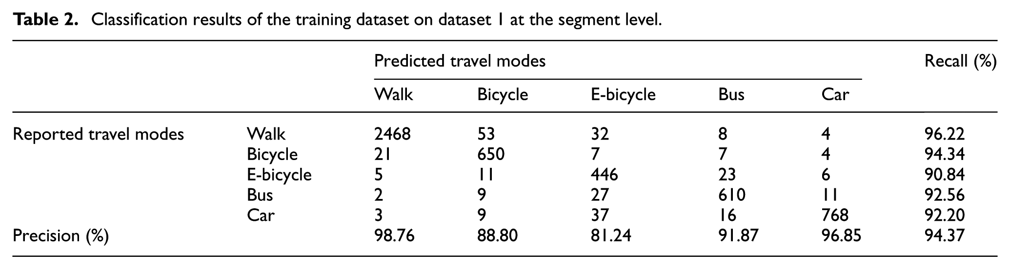
The confusion matrix of the training dataset and test dataset (as shown in Tables 2 and 3) is used to evaluate the performance of CHMMs. The accuracy is used to evaluate the overall classification performance, whereas the recall and precision are used to assess the classification performance of a given class.⁴⁶ As a whole, the accuracy exceeds 93% for both the training and test datasets, whereas the precision and recall are over 80% for each travel mode. In addition, the travel mode imputation of the test dataset achieves as high accuracy as that of the training dataset. Such a promising result demonstrates the powerful classification performance and prominent generalization of the CHMM.

Table 2.

Classification results of the training dataset on dataset 1 at the segment level.

		Predicted travel modes					Recall (%)
		Walk	Bicycle	E-bicycle	Bus	Car	Recall (%)
Reported travel modes	Walk	2468	53	32	8	4	96.22
	Bicycle	21	650	7	7	4	94.34
	E-bicycle	5	11	446	23	6	90.84
	Bus	2	9	27	610	11	92.56
	Car	3	9	37	16	768	92.20
Precision (%)		98.76	88.80	81.24	91.87	96.85	94.37

Table 3.

Classification results of the test dataset on dataset 1 at the segment level.

		Predicted travel modes					Recall (%)
		Walk	Bicycle	E-bicycle	Bus	Car	Recall (%)
Reported travel modes	Walk	818	22	10	5	2	95.45
	Bicycle	8	213	3	3	1	93.42
	E-bicycle	1	3	147	10	3	89.63
	Bus	0	3	9	198	6	91.67
	Car	2	2	14	7	255	91.07
Precision (%)		98.67	87.65	80.33	88.79	95.51	93.47

Further analysis on the precision of the travel modes in the test dataset can facilitate understanding of the advantages of CHMM in travel mode detection and the ways to improve the classification accuracy in future studies. Walk segments are imputed with the highest precision because walk modes have distinctive characteristics relative to other travel modes in terms of the average speed and the average absolute acceleration. More than 93% of the bicycle segments are detected correctly, possibly because the feature set includes the heading change rate that can effectively distinguish non-motorized segments from motorized segments. The precision for the bus and car modes exceeds 91%.

In practice, it is difficult to distinguish between bicycle and e-bicycle modes as well as between car and bus modes.^40,47 However, most falsely flagged bus segments are flagged as e-bicycle segments, rather than car segments, and vice versa. The low misidentification rate between car and bus segments may result from the application of the low-speed point rate. This low misidentification rate also indicates that this feature may take the place of a bus network to some extent. A low confusion rate also exists between bicycle and e-bicycle segments. This result may be associated with the inclusion of the heading change rate. In comparison, e-bicycle segments are imputed with the lowest precision possibly because of a great similarity between e-bicycle and bicycle modes in the average speed as well as between e-bicycle and bus modes in the average absolute acceleration. Thus, features with a high differentiation ability between e-bicycle and other modes need to be extracted in a future study.

Although travel modes are detected at the segment level, activity-based models generally require travel modes at the trip level. Therefore, an aggregation rule from segments to trips should be used to determine the main mode of the trip. According to the aggregation rules proposed by Axhausen,⁴⁸ the main mode is defined as the mode with the longest distance traveled, the longest duration, or the highest speed. In this study, the first rule is used, and the resulting aggregation results at the trip level are shown in Table 4. The classification accuracy of travel modes at the trip level is lower than that at the segment level for each mode. This scenario could be due to the incorrect detection for a segment with a main mode, which has a negative effect on trip mode accuracy. For example, a bus trip consists of a walk segment, a bus segment, and another walk segment. If the bus segment is falsely flagged, but the two walk segments are correctly detected, then the travel mode at the trip level will be classified incorrectly.

Table 4.

Classification results of the test dataset on dataset 1 at the trip level.

		Predicted travel modes					Recall (%)
		Walk	Bicycle	E-bicycle	Bus	Car	Recall (%)
Reported travel modes	Walk	253	8	4	1	0	95.11
	Bicycle	5	133	2	2	1	93.01
	E-bicycle	1	2	111	8	3	88.80
	Bus	0	2	8	105	6	86.78
	Car	2	2	13	6	224	90.69
Precision (%)		96.93	90.48	80.43	86.07	96.14	91.57

Comparison with other classifiers

Seven representative classifiers are used to impute travel modes, so that the relative performance of the CHMM is evaluated. These seven representative classifiers are SVM, multinomial logit (MNL), BN, artificial neural network (ANN), DHMM, dynamic BN (DBN), and Markov random field (MRF). The same training/test dataset is used, and the SFS procedure is used for each classifier, leading to comparable performance of these classifiers. The SVM classifier is constructed using a Gaussian kernel with package “e1071” (version: 1.6-7) in R, and the values of parameters are taken according to the recommendation by Zong et al.⁴⁹ Specifically, the cost of constraint violation (constant of the regularization term in the Lagrange formulation) is 84.54, whereas the free parameter in the Gaussian kernel is 0.7367. A one-versus-rest style is used to enable the multiclass classification. The MNL model is used with all the features as individual-specific attributes and base alternative as walk. This model does not incorporate specified weights and nets of features, and it is trained and tested with package “mlogit” (version: 0.2-4) in R. The structure of a BN classifier is determined with a K2 algorithm, and its conditional probability tables are computed with the maximum likelihood methods. Each feature is discretized as two to five equal parts, and the best discrete features are used based on the accuracy in test dataset. Structure and parameter learning, as well as inference, are implemented with package “bnlearn” (version: 4.0) in R. The ANN classifier is constructed with a three-layer neural network. Next, 1–20 neurons are tested for the hidden layer and the best performance is achieved with 13 neurons. The ANN classifier is trained with the back-propagation method, and the activation function uses a sigmoid form. The ANN classifier is implemented with a “neuralnet” package (version: 1.32) in R. Two to fifteen hidden states are tested using a DHMM, and each feature is discretized as two to five equal parts. Based on the results from all possible DHMMs, the best one is chosen according to the accuracy in test dataset. The training and test of these DHMMs are implemented with package “HMM” (version: 1.0) in R. Two to fifteen hidden states are used to maintain a consistent setting between CHMM and DBN by training the DBN. The commonly used feedback loop networks are used to train and test DBN. This classifier is implemented with package “ebdbNet” (version: 1.2.3) in R. Similar to the CHMM in this study, Gaussian distribution is used to train and test MRF. The resulting Gaussian MRF is implemented with package “RandomFields” (version: 3.1.10) in R.

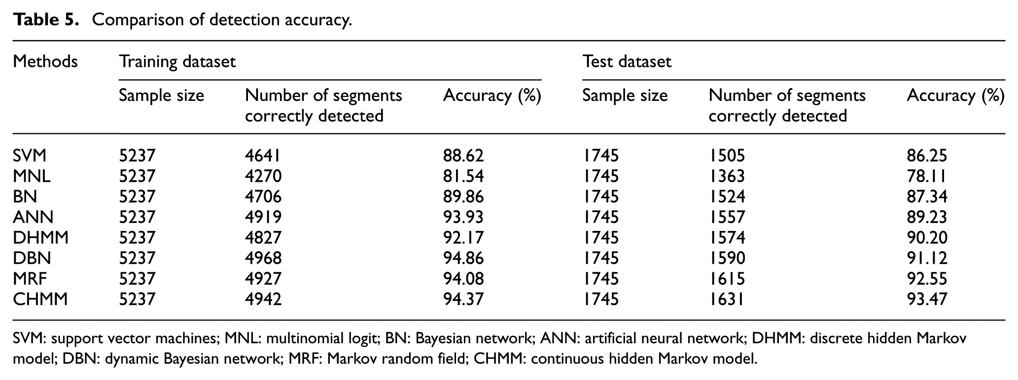
As shown in Table 5, the performance of classifiers is generally evaluated with the classification accuracy of the training and test dataset. The CHMM achieved the highest accuracy in both the training and test datasets. In fact, the relative classification accuracy of these classifiers is theoretically interpretable to a certain extent. Although the SVM classifier has excellent distinction ability by mapping feathers from a low-dimensional space to a high-dimensional one, it encounters challenge in its non-probabilistic classification output, denoting its inability to deal with ambiguity inherently involved in travel mode imputation. The MNL model is widely applied in the domain of travel behavior, but may be inappropriate for the travel mode imputation because the independence of irrelevant alternatives may fail. The BN classifier generally has a favorable classification ability, but it is more suitable to handle discrete features. The ANN classifier represents complex nonlinear relationships between independent and dependent variables, but is prone to overfitting in some cases. The accuracy in training and test dataset of DHMMs is lower than that of CHMMs, which may contribute to the relative advantage of CHMMs in terms of accuracy as compared with DHMMs. According to the classification results, the accuracy in training dataset of DBN is slightly higher than that of CHMMs. This scenario occurs possibly because a CHMM is a special case of the DBN family;⁵⁰ thus, flexibility and excellent fitting ability are incorporated by DBN.⁵¹ However, the prediction ability of DBN is lower than that of CHMMs. This scenario may result from a high flexibility and may result in an overfitting. MRF achieves the highest accuracy in test dataset among the seven benchmarks probably because of the MRF nature of the undirected graph, thereby enabling the distribution of a node to depend on its immediately previous node and on the next node. This is in line with the actual situation because mode transferability exists among neighboring segments when multiple travel modes are adopted sequentially during a tour. However, the estimation procedure of MRF deals with local minimization schemes, which implies the possibility of failing to achieve the global optimum.⁵²

Table 5.

Comparison of detection accuracy.

Methods	Training dataset			Test dataset
Methods	Sample size	Number of segments correctly detected	Accuracy (%)	Sample size	Number of segments correctly detected	Accuracy (%)
SVM	5237	4641	88.62	1745	1505	86.25
MNL	5237	4270	81.54	1745	1363	78.11
BN	5237	4706	89.86	1745	1524	87.34
ANN	5237	4919	93.93	1745	1557	89.23
DHMM	5237	4827	92.17	1745	1574	90.20
DBN	5237	4968	94.86	1745	1590	91.12
MRF	5237	4927	94.08	1745	1615	92.55
CHMM	5237	4942	94.37	1745	1631	93.47

SVM: support vector machines; MNL: multinomial logit; BN: Bayesian network; ANN: artificial neural network; DHMM: discrete hidden Markov model; DBN: dynamic Bayesian network; MRF: Markov random field; CHMM: continuous hidden Markov model.

This result demonstrates the reasonability of a CHMM in detecting travel modes. Furthermore, the CHMM achieved the smallest difference in the accuracy between training and test datasets. Therefore, the CHMM achieved better generalization than its competitors.

Classification results on dataset 2

The dataset 2 comprises a training dataset of 3042 segments and a test dataset of 1017 segments. Unlike the dataset 1, the dataset 2 includes the GSM/Wi-Fi data, which are not so accurate as GPS data, but can compensate for GPS signal loss or smooth the location data. In this study, the location data are pre-processed using a Kalman filter, which is used to derive accurate trajectories by combining the GSM/Wi-Fi data and the GPS data based on a linear motion model with the zero mean, Gaussian-distributed acceleration.²⁷

Accelerometer data consist of readings $(a_{x}, a_{y}, a_{z})$ in three directions. The $l_{2}$ norm $(f_{a} = | | a_{x}, a_{y}, a_{z} | | = \sqrt{a_{x}^{2} + a_{y}^{2} + a_{z}^{2}})$ of the readings are computed to obtain rotation invariant observations. Average, minimum, maximum, and standard deviation, coefficient of variance, and interquartile range of $f_{a}$ are introduced to the feature set. With the same method for feature selection as the dataset 1, average speed, standard deviation of $f_{a}$ , average absolute acceleration, low-speed point rate, and heading change rate are sequentially included to the optimal feature set for the dataset 2. The inclusion of standard deviation of $f_{a}$ as the second feature in the optimal feature set indicates the potential benefit of the accelerometer data in travel mode detection. Eight hidden states are included in the model with the highest accuracy in the test dataset on dataset 2. As shown in Table 6, the precision and recall are higher than the test dataset on dataset 1 for any travel mode. This indicates the necessity of detecting travel modes with the accelerometer data. In addition, the inclusion of the accelerometer data results in the highest increase in the recall for the walk mode. This is consistent with the conclusion reached by Feng and Timmermans.⁵³

Table 6.

Classification results of the test dataset on dataset 2 at the segment level.

		Predicted travel modes					Recall (%)
		Walk	Bicycle	E-bicycle	Bus	Car	Recall (%)
Reported travel modes	Walk	483	5	3	2	1	97.77
	Bicycle	3	126	2	1	0	94.74
	E-bicycle	0	2	89	5	2	90.82
	Bus	0	1	6	120	2	93.02
	Car	1	2	7	4	151	92.64
Precision (%)		99.18	92.65	83.18	90.91	96.79	95.28

Discussion and conclusion

The contribution of the article is summarized as follows. First, a travel survey with smartphones is conducted by a surveyor-involved PR survey with telephones. In this PR survey, the surveyor asks respondents to validate the travel information derived from the trajectory data, increasing the data quality of the ground truth. In the era of the artificial intelligence, the PR survey becomes a reliable approach to collect large-scale travel diaries adopted to train classification models for detecting travel modes. Second, SFS procedures are applied to select the most reasonable set of features, and they enable high classification accuracy with few features. The SFS procedures contribute to the alleviation of the overfitting issue that is often encountered in many classification tasks and the improvement of the computation time due to the reduction of features. Third, as a machine learning approach that incorporates high resistance to the noise in features, a CHMM is used to detect travel modes. The CHMM can take full advantage of information stored in the trajectories with smaller time windows, such as 1 or 2 min. The CHMM detects travel modes from a novel perspective by dividing a segment into a number of subsegments, which is obviously different from previous studies that only extract features at the segment level and neglect the possibility of improving classification accuracy by splitting a segment.

The CHMM with SFS procedures achieved an accuracy of 94.37% for the training dataset and 93.47% for the test dataset on dataset 1. In addition, 95.28% of segments are detected correctly in the test dataset on dataset 2. The promising results obtained with this method provides a novel perspective in travel mode detection and other related issues in GPS travel surveys, including trip purpose detection. Compared with other commonly used methods, the CHMM achieved the highest classification accuracy and exhibited a favorable generalization. From the perspective of empirical studies, the CHMM also has an advantage over other similar efforts. Zheng et al.⁵⁴ used decision trees to differentiate walk, bicycle, car, and bus modes and correctly classify 75.6% of samples. Tsui and Shalaby⁵⁵ used fuzzy logic method to detect these four travel modes, and high accuracy of 91% was achieved.

The CHMM has a bright prospect of imputing travel modes in a smartphone-based travel survey. As smartphones become increasingly popular, smartphone-based travel surveys are expected to become more attractive because they can decrease the burden of respondents and improve the data quality using a PR survey. The improvement of the automation in travel surveys also emphasizes the role of classifiers with high classification accuracy. In a future study, we need to extract features that achieve high distinction between e-bicycle segments and segments with other modes because of the relatively low precision in detecting e-bicycle segments.

Footnotes

Handling Editor: Daming Zhou

Declaration of conflicting interests

The author(s) declared no potential conflicts of interest with respect to the research, authorship, and/or publication of this article.

Funding

The author(s) disclosed receipt of the following financial support for the research, authorship, and/or publication of this article: This research is supported by the National Natural Science Foundation of China (51478266).

ORCID iD

Guangnian Xiao

References

Downs

The law of peak-hour expressway congestion. Traffic Quart 1962; 16(3): 347–362.

Rotaris

Danielis

Commuting to college: the effectiveness and social efficiency of transportation demand management policies. Transp Policy 2015; 44: 158–168.

Rotaris

Danielis

The impact of transportation demand management policies on commuting to college facilities: a case study at the University of Trieste, Italy. Transp Res Part A Policy Pract 2014; 67: 127–140.

Clifton

Currans

Cutter

et al . Household travel surveys in context-based approach for adjusting ITE trip generation rates in urban contexts. J Transp Res Board 2012; 2307: 108–119.

Prelipcean

Gidófalvi

Susilo

YO.

MEILI: a travel diary collection, annotation and automation system. Comput Environ Urban Syst 2018; 70: 24–34.

Wagner

Lexington area travel data collection test: GPS for personal travel surveys. Columbus, OH: Office of Highway Policy Information and Office of Technology Applications, Federal Highway Administration, Battelle Transport Division, 1997.

Kelly

Krenn

Titze

et al . Quantifying the difference between self-reported and global positioning systems-measured journey durations: a systematic review. Transp Rev 2013; 33(4): 443–459.

Zong

Tang

et al . Identifying activities and trips with GPS data. IET Intell Transp Syst 2018; 12(8): 884–890.

Ermagun

Fan

Wolfson

et al . Real-time trip purpose prediction using online location-based search and discovery services. Transp Res Part C Emerg Technol 2017; 77: 96–112.

10.

Van Dijk

. Identifying activity-travel points from GPS-data with multiple moving windows. Comput Environ Urban Syst 2018; 70: 84–101.

11.

Procter

Page

Cooper

et al . An open-source tool to identify active travel from hip-worn accelerometer, GPS and GIS data. Int J Behav Nutr Phys Act 2018; 15(1): 91–100.

12.

Yang

Stewart

Tang

et al . A review of GPS trajectories classification based on transportation mode. Sensors 2018; 18(11): E3741.

13.

Feng

Timmermans

. Comparison of advanced GPS data imputation algorithms for detection of transportation mode and activity episode. In: Proceedings of the Transportation Research Board 93rd annual meeting, Washington, DC, 12–16 January 2014. Washington, DC: Transportation Research Board.

14.

Maruyama

Mizokami

Hato

. A smartphone-based travel survey trial conducted in Kumamoto, Japan: an examination of voluntary participants’ attributes. In: Proceedings of the Transportation Research Board 93rd annual meeting, Washington, DC, 12–16 January 2014. Washington, DC: Transportation Research Board.

15.

Cottrill

Pereira

Zhao

et al . Future mobility survey: experience in developing a smartphone-based travel survey in Singapore. J Transp Res Board 2013; 2354: 59–67.

16.

Stopher

Fitzgerald

Assessing the accuracy of the Sydney household travel survey with GPS. Transportation 2007; 34(6): 723–741.

17.

Bermingham

Pong-Wong

Spiliopoulou

et al . Application of high-dimensional feature selection: evaluation for genomic prediction in man. Sci Rep 2015; 5: 1–12.

18.

Hagenauer

Helbich

A comparative study of machine learning classifiers for modeling travel mode choice. Expert Syst Appl 2017; 78: 273–282.

19.

Reddy

Mun

Burke

et al . Using mobile phones to determine transportation modes. ACM T Sensor Netw 2010; 6(2): 13.

20.

Stenneth

Wolfson

et al . Transportation mode detection using mobile phones and GIS information. In: Proceedings of the 19th SIGSPATIAL international conference on advances in geographic information systems, Chicago, IL, 1–4 November 2011. New York: ACM.

21.

Xiao

Juan

Gao

Detecting travel modes using particular rules combined with a Naïve Bayesian classifier. In: Proceedings of the Transportation Research Board 94th annual meeting, Washington, DC, 11–15 January 2015. Washington, DC: Transportation Research Board.

22.

Schuessler

Axhausen

KW.

Processing raw data from global positioning systems without additional information. J Transp Res Board 2009; 2105(1): 28–36.

23.

Liao

Fox

Kautz

Extracting places and activities from GPS traces using hierarchical conditional random fields. Int J Robot Res 2007; 26(1): 119–134.

24.

Troped

Oliveira

Matthews

et al . Prediction of activity mode with global positioning system and accelerometer data. Med Sci Sports Exer 2008; 40(5): 972–978.

25.

Zhou

Al-Durra

Gao

et al . Online energy management strategy of fuel cell hybrid electric vehicles based on data fusion approach. J Power Sources 2018; 366: 278–291.

26.

Parlak

Jariyasunant

Sengupta

. Using smartphones to perform transportation mode determination at the trip level. In: Proceedings of the Transportation Research Board 91st annual meeting, Washington, DC, 22–26 January 2012. Washington, DC: Transportation Research Board.

27.

Nitsche

Widhalm

Breuss

et al . Supporting large-scale travel surveys with smartphones–a practical approach. Transp Res Part C Emerg Technol 2014; 43: 212–221.

28.

Beyreuther

Wassermann

Continuous earthquake detection and classification using discrete hidden Markov models. Geophys J Int 2008; 175(3): 1055–1066.

29.

Melnikoff

Quigley

Russell

MJ.

Speech recognition on an FPGA using discrete and continuous hidden Markov models. In: Glesner

Zipf

Renovell

(eds) Field-programmable logic and applications: reconfigurable computing is going mainstream. Berlin: Springer, 2002, pp.202–211.

30.

Zhou

Al-Durra

Zhang

et al . Online remaining useful lifetime prediction of proton exchange membrane fuel cells using a novel robust methodology. J Power Sour 2018; 399: 314–328.

31.

Rigoll

Kosmala

Rattland

et al . A comparison between continuous and discrete density hidden Markov models for cursive handwriting recognition. In: Proceedings of the 13th international conference on pattern recognition, Vienna, 25–29 August 1996. New York: IEEE.

32.

Alma’adeed

Higgins

Elliman

Off-line recognition of handwritten Arabic words using multiple hidden Markov models. In: Coenen

Preece

Macintosh

(eds) Research and development in intelligent systems. London: Springer, 2004, pp.33–40.

33.

Ghorpade

Pereira

Zhao

et al . An integrated stop-mode detection algorithm for real world smartphone-based travel survey. In: Proceedings of the Transportation Research Board 94th annual meeting, Washington, DC, 11–15 January 2015. Washington, DC: Transportation Research Board.

34.

Bieber

Kirste

Gaede

. Low sampling rate for physical activity recognition. In: Proceedings of the 7th international conference on pervasive technologies related to assistive environments, Rhodes, 27–30 May 2014. New York: ACM.

35.

Greaves

Fifer

Ellison

et al . Development of a global positioning system web-based prompted recall solution for longitudinal travel surveys. J Transp Res Board 2010; 2183(1): 69–77.

36.

Wilhelm

Wolf

Oliveira

et al . Application of GPS-based prompted recall methods in two household travel surveys. In: Proceedings of the Transportation Research Board 91st annual meeting, Washington, DC, 22–26 January 2012. Washington, DC: Transportation Research Board.

37.

Pereira

Carrion

Zhao

et al . The future mobility survey: overview and preliminary evaluation. In: Proceedings of the Eastern Asia Society for Transportation Studies, Kawana, Japan, 9–12 September 2013. Tokyo, Japan: Eastern Asia Society for Transportation Studies.

38.

Gong

Kanamori

Yamamoto

Data selection in machine learning for identifying trip purposes and travel modes from longitudinal GPS data collection lasting for seasons. Travel Behav Soc 2017; 11: 131–140.

39.

Gonzalez

Weinstein

Barbeau

et al . Automating mode detection for travel behaviour analysis by using global positioning systems-enabled mobile phones and neural networks. IET Intell Transp Syst 2010; 4(1): 37–49.

40.

Broach

Mcneil

Dill

Travel mode imputation using GPS and accelerometer data from a multi-day travel survey. In: Proceedings of the Transportation Research Board 93rd annual meeting, Washington, DC, 12–16 January 2014. Washington, DC: Transportation Research Board.

41.

Zhou

Nguyen

Breaz

et al . Global parameters sensitivity analysis and development of a two-dimensional real-time model of proton-exchange-membrane fuel cells. Energ Convers Manage 2018; 162: 276–292.

42.

Zhou

Al-Durra

Matraji

et al . Online energy management strategy of fuel cell hybrid electric vehicles: a fractional-order extremum seeking method. IEEE T Ind Electron 2018; 65(8): 6787–6799.

43.

Chen

et al . Identifying travel mode from GPS trajectories through fuzzy pattern recognition. In: Proceedings of the 7th international conference on the fuzzy systems and knowledge discovery, Yantai, China, 10–12 August 2010. New York: IEEE.

44.

Jelinek

Bahl

Mercer

Design of a linguistic statistical decoder for the recognition of continuous speech. IEEE T Inform Theory 1975; 21(3): 250–256.

45.

Norvig

Russell

Artificial intelligence: a modern approach. Upper Saddle River, NJ: Prentice-Hall, 1995, pp.25–27.

46.

Powers

DM.

Evaluation: from precision, recall and F-measure to ROC, informedness, markedness and correlation. J Mach Learn Technol 2011; 2(1): 37–63.

47.

Stopher

Jiang

FitzGerald

Processing GPS data from travel surveys. In: Proceedings of the 2nd international colloqium on the behavioural foundations of integrated land-use and transportation models: frameworks, models and applications, Toronto, ON, Canada, June 2005, https://atrf.info/papers/2005/2005_Stopher_Jiang_FitzGerald.pdf

48.

Axhausen

KW.

Definition of movement and activity for transport modelling. In: Hensher

Button

(eds) Handbooks in transport: transport modelling. Oxford: Pergamon Press, 2000, pp.4–7.

49.

Zong

Bai

Wang

et al . Identifying travel mode with GPS data using support vector machines and genetic algorithm. Information 2015; 6(2): 212–227.

50.

Ghahramani

An introduction to hidden Markov models and Bayesian networks. Int J Pattern Recogn Artif Intell 2001; 15(1): 9–42.

51.

Liao

Patterson

Fox

et al . Learning and inferring transportation routines. Artif Intell 2007; 171(5): 311–331.

52.

José

La Rosa

González

et al . A comparative study of some Markov random fields and different criteria optimization in image restoration. London: IntechOpen Access Publisher, 2012.

53.

Feng

Timmermans

HJ.

Transportation mode recognition using GPS and accelerometer data. Transp Res Part C Emerg Technol 2013; 37: 118–130.

54.

Zheng

Chen

et al . Understanding transportation modes based on GPS data for web applications. ACM T Web 2010; 4(1): 1–36.

55.

Tsui

SYA

Shalaby

. Enhanced system for link and mode identification for personal travel surveys based on global positioning systems. J Transp Res Board 2006; 1972(1): 38–45.

Detecting travel modes from smartphone-based travel surveys with continuous hidden Markov models

Abstract

Keywords

Introduction

Data collection and description

Respondent instruction

Data validation

Data description

Feature extraction and selection

Feature extraction

Feature selection

Travel mode detection with CHMMs

CHMMs

Model training with the training dataset

Classification with the test dataset

Classification results on dataset 1

Comparison with other classifiers

Classification results on dataset 2

Discussion and conclusion

Footnotes

Declaration of conflicting interests

Funding

ORCID iD

References