Recognizing human activities from smartphone sensors using hierarchical continuous hidden Markov models

Abstract

Human activity recognition has been gaining more and more attention from researchers in recent years, particularly with the use of widespread and commercially available devices such as smartphones. However, most of the existing works focus on discriminative classifiers while neglecting the inherent time-series and continuous characteristics of sensor data. To address this, we propose a two-stage continuous hidden Markov model framework, which also takes advantage of the innate hierarchical structure of basic activities. This kind of system architecture not only enables the use of different feature subsets on different subclasses, which effectively reduces feature computation overhead, but also allows for varying number of states and iterations. Experiments show that the hierarchical structure dramatically increases classification performance. We analyze the behavior of the accelerometer and gyroscope signals for each activity through graphs, and with added fine tuning of states and training iterations, the proposed method is able to achieve an overall accuracy of up to 93.18%, which is the best performance among the state-of-the-art classifiers for the problem at hand.

Keywords

Human activity recognition smartphone sensors accelerometer gyroscope continuous hidden Markov model hierarchical classifier

Introduction

The past decade has opened up the development of a wide range of sensors and mobile devices with unprecedented characteristics. The exceptional efficiency, portability, and affordability of these devices naturally extended their availability to a more diverse number of people.¹ More specifically, the number of smartphone users worldwide is expected to catapult to 1.75 billion in 2014, having only reached the 1 billion mark last 2012. As a result, more and more people have come to rely on and interact with these devices as part of their normal daily lives.

These events bring about a great number of possibilities. On top of various applications using smartphone sensors such as Bluetooth-aided mobile phone localization and distributed range-free localization of wireless sensor networks, the use of sensors to recognize human activities has sparked a lot of research interest due to its promising applications in the areas of pervasive and mobile computing, surveillance-based security, ambient assistive living, and context-aware computing.² Activity recognition has also made its debut recently as the key component on several consumer products such as Nintendo Wii and Microsoft Kinect.³ Although they were originally made for the purpose of gaming and entertainment, these systems have attracted additional applications, such as personal fitness training and rehabilitation, and have also brought about further research in human activity recognition (HAR).^4,5

In addition to this, smartphone sensor technologies are developing at an incredible pace. Various context-related sensors are now normally embedded into mobile phones, such as Global Positioning System (GPS), Wi-Fi, Bluetooth, accelerometers, magnetometers, gyroscopes, barometers, proximity sensors, temperature and humidity sensors, ambient light sensors, cameras, and microphones.⁶ With the unmistakable prevalence of the smartphone, together with its variety of readily available sensors, it is only natural to exploit such a mass-marketed device to be able to automatically recognize human daily activities without imposing inconveniences to the user.⁷

Most research works in activity recognition have focused on using discriminative approaches such as support vector machines (SVM) and decision trees, neglecting the time-series component of sensor signals. Although these models are light-weight, they are systems that require the use of a rich set of features, which in turn increases computational costs, in exchange for algorithm simplicity.^3,8–10 To take advantage of this inherent characteristic of sensor signals, particularly from the accelerometer and gyroscope of a smartphone, we propose a temporal probabilistic approach to activity recognition. A hidden Markov model (HMM) is a Markov chain with both hidden and unhidden stochastic processes. Thus, for the context of activity recognition, the unhidden or observable components are the sensor signals, while the hidden element is the user’s activity. There are several researchers to utilize HMM for activity recognition, but most of them are based on discrete HMM that only fits to the static images of data. However, since signals are inherently real-valued and it may incur loss of relevant detailed information to convert them to discrete values,¹¹ we exploited continuous hidden Markov models (CHMMs) for the task.

Activities are inherently hierarchical,¹² that is, a person has to be stationary in order for him to be considered standing (ST), or that a low-level activity like sitting (SI) is generally the position of a person who is doing a high-level activity like eating. We make use of this simple knowledge and employ a hierarchical architecture of CHMMs to recognize activities. This kind of system architecture also enables us to use different feature sets for different stages, of which random forest (RF) variable importance (VI) measures are utilized for feature selection. We show that RF VI measures are more accurate in identifying the most important variables (In the field of pattern recognition, the terminology of variable is interchangeably used with feature. In this article, we also use them several times with the same meaning.) compared to other feature selection methods, the hierarchical structure of the proposed method significantly improves activity classification performance and allows the usage of a varying number of states in the same subclass, as well as a varying number of training iterations for each activity of CHMM. Main contribution of this work lies in proposing a natural and maybe popular classifier architecture of CHMMs for better performance for this problem at hand.

Related works

One of the most cited works on HAR is the one by Bao and Intille.¹³ Data were collected from 20 users, each wearing five biaxial accelerometers placed on strategic parts of the body. An accuracy of around 80% was obtained after classifying 20 different activities using simple decision trees and fast Fourier transform (FFT)-based features. The work also specifically indicated that the sensors placed on the individual’s thigh and dominant hand take the most important role in recognizing activities. Other recent works also reinforced this claim.^14,15

In addition to Bao and Intilles’ work, there are several other studies which focused on using multiple accelerometers to perform activity recognition.^16,17 However, this approach is evidently inconvenient and somewhat obtrusive to the user besides being less accurate compared to using only a single strategically placed accelerometer.¹⁵

There are also some works which used a single tri-axial accelerometer. Using a single wrist-worn accelerometer, Chernbumroong et al.¹⁸ recognized five basic activities with 13 time- and frequency-based features using decision trees. Another work placed the accelerometer on the subject’s waist to recognize six basic activities using k-nearest neighbors and naïve Bayes classifiers.¹⁹ Sharma et al.²⁰ used neural networks, while Khan used the Wii Remote to classify basic activities.⁴ These works have indeed achieved high accuracies with their proposed set of simple features and classifiers, but note that they did not include two basic activities that are a little bit more difficult to classify—upstairs and downstairs movements—a factor which had a considerable contribution to their high results. Rubaiyeat et al.,²¹ however, included the aforementioned movements and achieved lower accuracy than previous works by Chernbumroong et al.¹⁸ and Gupta and Dallas.¹⁹

Other earlier published works have already made use of commercially available devices such as smartphones. Yang²² used a Nokia N95 mobile phone’s accelerometer with decision trees and HMM to classify six activities. Kwapisz et al.²³ used an Android smartphone’s single tri-axial accelerometer placed on the user’s pants pocket to recognize six basic activities using three different classifiers. However, the former also excluded upstairs and downstairs movements, while the latter failed to achieve high accuracy on upstairs and downstairs movements. It is interesting to note that the former particularly suggested the use of HMMs in order to capture more temporal correlations in the model. Moreover, this also shows that data from the accelerometer are not enough to efficiently differentiate between upstairs and downstairs movements.

Various other sensors were also investigated when used together with the accelerometer. Wu et al. concluded that the addition of the gyroscope is very beneficial, while Shoaib et al. fortified the claim that accelerometers and gyroscopes are not only efficient when used alone but also significantly improves classification performance when used on top of each other.

HMMs have been widely applied in the field of activity recognition in conjunction with multiple accelerometer sensors. Olguin and Pentland²⁶ made use of three tri-axial accelerometers placed on right-wrist, left-hip, and chest to classify eight basic activities (excluding upstairs and downstairs movements). Their system achieved around 92% overall accuracy and suggested to model each activity with a different number of hidden states. Travelsi et al.²⁷ considered an unsupervised learning approach using multiple HMM regression. They used three accelerometers placed on the chest, thigh, and ankle to recognize six activities, including upstairs and downstairs movement, and achieved around 91% classification accuracy. Mannini and Sabatini²⁸ obtained the data set gathered by Bao and Intille, extracted and used a sub-dataset to classify seven basic activities (including upstairs movement), and obtained a very high accuracy for CHMMs.

Khan et al.²⁹ applied a hierarchical neural network recognizer to classify 15 static, transitional, and dynamic activities using their proposed augmented feature vectors and obtained exceptionally high results. Our previous work,³⁰ involving the recognition of low- and high-level activities, successfully made use of hierarchical HMMs, albeit the difficulty in differentiating upstairs and downstairs movements. Multi-stage system architectures in conjunction with HMMs have also been successfully implemented in different application domains, such as attack and intrusion detection, gesture recognition, and smart home environments.^31–33

Finally, our previous work,³⁴ which incorporates multi-staged CHMMs for activity recognition using the accelerometer and gyroscope, is extended through a more comprehensive experimentation and analysis method—CHMM states were varied in each subclass, and the effect of gradually increasing Baum–Welch (BW) iterations is examined.

The proposed method

The proposed method is composed of a hierarchical structure of CHMMs (as seen in Figure 1). This kind of architecture enables us to exploit the inherent hierarchical characteristics of activities,¹² while CHMMs are advantageous to use with continuous observation densities such as sensor signals.²⁴ Moreover, feature selection is performed through utilizing RF VI measures since RF VI works significantly well with continuous, possibly highly correlated variables.²⁵ The hierarchical structure also enables us to use different feature subsets for different subclasses while minimizing feature computation time.

Figure 1.

The proposed hierarchical structure in conjunction with CHMMs.

Feature selection using RF VI measures

RF is an ensemble classification method pioneered by L Breiman. This technique is the result of combining bagging and random feature selection, creating a collection of simple decision trees, T = h(x,Θ_k), k = 1, …, K, where {Θ_k} are independent, identically distributed random vectors, that perform the task of classification by voting for the most popular class at input x, that is

p (c | v) = \frac{1}{T} \sum_{t = 1}^{T} p_{t} (c | v)

(1)

where p(c|v) is the average classification output of all the trees T, v is the bootstrapped data, and c is the class. The ensemble method can be used to obtain useful estimates, VI.³⁵

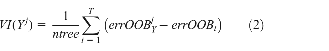
The first step to computing VI is fitting the training data into a RF model, followed by the computation of the out-of-bag (OOB) error at each data point in the forest. With the use of random data sampling, out-of-bagging is performed by leave-one-out cross validation, where data points are randomly permuted in an OOB_Y sample, to get the perturbed sample OOB_Y^j. The error of variable Y is calculated through the perturbed and unperturbed samples, and the summation of their difference is averaged over the total number of trees in the forest, ntree, obtaining the VI of Y, given by

VI (Y^{j}) = \frac{1}{ntree} \sum_{t = 1}^{T} ({errOOB}_{Y}^{j} - errOO B_{t})

(2)

The scores are then normalized with the standard deviation.

Hierarchical CHMMs

HMM is a doubly embedded stochastic process, composed of an unobservable stochastic process (hidden) and another set of stochastic processes that produces the sequence of observations—which is the only avenue to be able to observe the hidden one. It is most suitable in modeling time-series data such as those that can be found in speech recognition and signal processing applications.²⁴

The problem arises when, in applications such as activity recognition through signals (or vectors) produced by sensors, observations are continuous. Although it is definitely possible to quantize these signals into discrete symbols, it is undeniable that there will be serious degradation after the quantization process. Therefore, for such applications, it is advantageous to use HMMs with continuous observation densities.²⁴

If the observed process {Y_n| n ∈ N} is real-valued or vector-valued in a Euclidean space $O \subseteq ℜ^{d}$ , the pair of processes X_n, which is the unobserved process, and Y_n is called a CHMM. A CHMM is characterized by the number of states N, where S = {S₁, S₂, …, S_N} as the individual states and q_t is the state at time t, π is the initial state distribution, A is the state transition probability distribution, and B is the observation probability distribution, that is

λ = (A, B, π)

(3)

The initial probability distribution π = {π_i} is denoted by

π_{i} = P [q_{1} = S_{i}], 1 \leq i \leq N

(4)

while the state transition probability distribution A is indicated by the matrix {a_ij} where

a_{i j} = P [q_{t + 1} = S_{j} | q_{t} = S_{i}], 1 \leq i, j \leq N

(5)

For a CHMM, the observation probability distribution B corresponds to a family of parametric probability density functions (pdfs) ${p_{Y} (\cdot; θ), θ \in Θ}$ and a matrix B = (θ₁, θ₂, …, θ_M), in which M is the number of elements of $Θ \subseteq ℜ^{p}$ such that

F_{Y | X} (ϕ | i) = \int_{- \infty}^{ϕ} p_{Y} (y; θ_{i}) dy

(6)

where $p_{Y} (y; θ_{i})$ is the emission density of state i. The emission densities can also be denoted as

b_{i} (y) = p_{Y} (y; θ_{i}) = f (y; θ_{i}), i \in S, y \in O

(7)

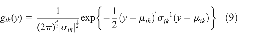
which is the same as a pdf. The parametric model for CHMM emission densities used in this work is the finite mixture of Gaussian pdfs, given by

f (y; θ_{i}) = \sum_{k = 1}^{K_{i}} v_{ik} g_{ik} (y), y \in ℜ^{d}

(8)

where v_ik is the mixture coefficient for the kth mixture in state i and

g_{ik} (y) = \frac{1}{{(2 π)}^{\frac{d}{2}} | σ_{ik} |^{\frac{1}{2}}} \exp {- \frac{1}{2} {(y - μ_{ik})}^{'} σ_{ik}^{- 1} (y - μ_{ik})}

(9)

The mixture gains should satisfy the stochastic constraints

\sum_{k = 1}^{K_{i}} v_{ik} = 1, 1 \leq i \leq N

(10)

v_{ik} \geq 0, 1 \leq i \leq N, 1 \leq k \leq K

(11)

so that the pdf is properly normalized.

The proposed method is divided into two stages: the first level, which categorizes activities into Dynamic or Static subclasses, and the second level, which outputs the final activity class C = {Walking, W; Walking Upstairs, WU; Walking Downstairs, WD; Sitting, SI; Standing, ST; Laying, L}, where {W, WU, WD} ∈ Dynamic; {SI, ST, L} ∈ Static.

The BW algorithm is a special case of the expectation maximization (EM) algorithm, which is used to adjust the model parameters (A, B, π) in order to maximize the probability of a given observation sequence, O = O₁O₂…O_T, given the model λ, that is, P(O|λ). Using the iterative procedure of the algorithm, we re-estimate the current model λ to find a new model $\bar{λ} = (\bar{A}, \bar{B}, \bar{π})$ from which O is more likely to have been produced, given that $P (O | \bar{λ}) > P (O | λ)$ . Likewise, maximizing Baum’s auxiliary function

Q (λ | \bar{λ}) = \sum_{Q} P (Q | O, λ) \log [P (O, Q | \bar{λ})]

(12)

over $\bar{λ}$ will get

max_{\bar{λ}} [Q (λ, \bar{λ})] \Rightarrow P (O | \bar{λ}) \geq P (O | λ)

(13)

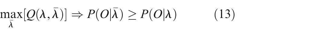
which yields an increase in likelihood. Iteratively, using $\bar{λ}$ in place of λ and repeating the re-estimation calculation, the probability of O being produced by the model can be improved, until some limiting point is reached (maximum likelihood estimate of a CHMM). As we will see later, there is a peak in the number of BW iterations in which the resulting CHMM is said to be generalized and not overfitted.

Figure 2(a) shows how the first-level CHMMs are trained. Acceleration and gyroscopic data are preprocessed, which include scaling and feature selection by RF, and fed to first-level CHMMs for training. CHMMs on this level have two states, corresponding to the number of classes or activities to be classified at a certain instance.^17,19 A two-state CHMM is denoted by the pdf

P_{Y} (y; θ_{i}) = = \frac{1}{\sqrt{2 π σ_{i}^{2}}} \exp {- \frac{{(y - μ_{i})}^{2}}{2 σ_{i}^{2}}}

(14)

where θ_i = (µ_i, σ_i) and i = 1, 2 (two states). All Dynamic training data are fed to the dynamic CHMM, while all Static training data are directed to the static CHMM. Thus, for each subclass e ∈ E, a resulting trained CHMM λ_e is created.

Figure 2.

Training of (a) first-level and (b) second-level CHMMs.

Conversely, CHMMs on the second level will first have three states,^17,19 but these states will be varied to examine its effect on classification performance.²⁶ Training for this level is also different from the first level such that CHMMs for Dynamic activities use a completely different feature subset from CHMMs for Static activities. For each subclass, we build a CHMM λ_ed for each dynamic activity and λ_es for each static activity and estimate the model parameters (A, B, π)_d and (A, B, π)_s, respectively, that optimize the likelihood of the corresponding training observations (as seen in Figure 2(b)).

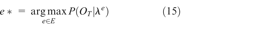
Given the trained models resulted from repeated iterations of BW, new data, which are processed to produce the same feature subset as the corresponding training data, are classified into Dynamic and Static subclasses on the coarse classification stage (as seen in Figure 3(a)). Thus, given a trained CHMM λ^e and a feature subset of new data O_T, we estimate the likelihood of the observation O_T belonging to first-level subclass e ∈ E. Using the relationship P(O_T|λ^e) estimated across all CHMMs in this level, we select the activity with the highest probability given by

e * = \underset{e \in E}{\arg max} P (O_{T} | λ^{e})

(15)

Figure 3.

(a) First-level CHMMs for coarse classification and (b) second-level CHMMs for fine classification.

The forward–backward algorithm is used to compute P(O_T|λ^e), as shown in Figure 4. Given a forward variable

α_{t} (i) = P (O_{1} O_{2} \dots O_{t}, q_{t} = S_{i} | λ)

(16)

which is the same as the probability of the partial observation sequence, O₁O₂…O_t and state S_i at time t, given the model λ^e, P(O_T|λ^e) can be computed by first initializing the forward probabilities as the joint probability of state S_i and first observation O₁

α_{1} (i) = π_{i} b_{i} (O_{1}), 1 \leq i \leq N

(17)

that is, the first row on every α table in Figure 4. The forward probability of reaching state S_j at time t + 1 from N possible states S_i, i = {1, 2, …, N}, at time t is

α_{t + 1} (j) = [\sum_{i = 1}^{N} α_{t} (i) a_{ij}] b_{j} (O_{t + 1}), \begin{matrix} 1 \leq t \leq T - 1 \\ 1 \leq j \leq N \end{matrix}

(18)

where α_t(i)a_ij is the probability of the joint event that O₁O₂…O_t are observed, and state S_i is reached at time t + 1 via state S_i at time t. The summation of these joint probabilities over all possible N states at time t is the probability of S_j at time t + 1, with all the previous partial observations included. The forward probability at time t + 1 can then be computed by multiplying the summed quantity by the probability accounting for observation O_t +₁ in state j, b_j(O_t +₁).

Figure 4.

The forward–backward algorithm for determining the class e of a given observation sequence O_seq.

Equation (18) is repeatedly performed for all states j at a given time t, and this process is performed recurrently for all t = 1, 2, …, T − 1. Thus, we arrive at the probability of the observation O_T, given the model λ^e, given by

P (O_{T} | λ^{e}) = \sum_{i = 1}^{N} α_{T} (i)

(19)

where α_T(i) is the forward terminal variable at state i.

Once activities are categorized according to their respective subclasses on the first level, we then proceed to classify test data into their corresponding activity, C = {W, WU, WD, SI, ST, L}.⁹ This is done by fine classification on the second level.

Given the test feature subset that was categorized in the previous level, now O_T^d and O_T^s, the forward–backward algorithm is again used to determine the activity with the highest probability e_d* and e_s* for the dynamic and static subclasses, respectively (as seen in Figure 3(b)).

Experiments

HAR data set

The publicly available UC Irvine (UCI) HAR data set was used throughout our experiments.⁹ This data set is composed of accelerometer and gyroscope normalized data values gathered from a Samsung Galaxy S II smartphone worn on the waist by 30 subjects performing a protocol of activities at 50 Hz. The data set also includes 561 features computed from 50% overlapped sliding windows, each window being 2.56 s in length. It is partitioned into 70% training data (from 21 subjects chosen randomly) and 30% test data (from the remaining 9 subjects).

Exploratory analysis and scaling

Figure 5 shows the correlation heat maps of accelerometer and gyroscope inertial values from subject 1. As can be observed from the graph, W is significantly different from WU and WD and thus can be easily separated during classification. However, WU and WD have very similar accelerometer correlation plots, while their gyroscope heat maps are noticeably different. This clearly illustrates the need for the gyroscope to distinguish between the two very similar activities.

Figure 5.

Correlation heat maps of sensor inertial values for each activity.

From the heat plots of SI, ST, and L, it is evident that their acceleration values are enough to easily set them apart. We will see later that these simple observations will clearly manifest in the feature subsets derived using RF.

By considering equations (16)–(18), and knowing that each a and b term is usually significantly less than 1, one can observe that as t starts to become larger and larger (in the case of long observation sequences), α_t(i) starts to head exponentially to zero. The only way to prevent this underflow phenomenon from happening is by scaling.²⁴

Examining the out-of-the-box HAR data set, values are normalized but not z-scaled, that is, the variables do not have a mean of approximately zero and a standard deviation of 1. Scaling is performed by extracting z-scores (standardized scores) for each variable Y_n, given by

z = \frac{Y_{n} - μ}{σ}

(20)

where z is the scaled value, µ is the mean of all data points in variable Y_n, and σ is the standard deviation of all variable points.

Feature selection using RF VI

The whole feature data set, consisting of 561 variables, is fitted to an RF model 50 times to obtain the average VI measure for each variable per activity.³⁶ Predictors with VI values higher than the mean VI of all predictors are retained and ranked in descending order, producing a feature subset of Y_1:m + 1 variables. Using CHMM as the wrapper algorithm, a combination of step-wise and 10-fold cross-validation procedure is performed to create multiple models λ_m, m ∈ M, starting from the two most important variables Y_1:2 (which produces λ₁) and ending with the feature subset including all Y_1:m + 1 variables (which produces the final model λ_m as seen in Figure 6). The variables of the model with the least error rate are then adopted to become the feature subset for the coarse classification stage, F₀. Figure 7 shows that the model with the lowest error rate was obtained after the addition of the 119th variable; thus, the first-level feature subset F₀ consists of these 119 variables.

Figure 6.

The step-wise cross-validation procedure.

Figure 7.

Error rates of first-level CHMM per the number of features.

Upon examination of the resulting feature subset, it is apparent in the per-activity VI values that the features with high VI for Dynamic activities have substantially low VI for Static activities. Thus, it is clear that the separation of Dynamic and Static activities into subclasses is beneficial so as not only to boost classification performance but also to minimize feature computation cost by using fewer variables for each second-level subclass.

The second-level feature subsets, F_D and F_S, are derived from the first-level subset. As discussed earlier, F_D should contain less accelerometer-based features (since gyroscope-based features are more beneficial for the Dynamic subclass) compared to the F₀. By performing the same step-wise cross-validation procedure as F₀ for each subclass, the resulting dynamic subset F_D and static subset F_S were produced, the former consisting of 95 less accelerometer-based variables, while the latter consisting of five accelerometer-based variables. Note that the majority of F_D features and all five features of F_S are time-based; this is important since total energy overhead when generating time-based features is significantly lower than when generating frequency-based ones, especially since the activity recognition platform is a smartphone with limited battery life.³⁷

To compare our feature selection method with other commonly used dimension reduction techniques, we derived feature subsets using correlation,³⁸ principal component analysis (PCA),³⁹ and step-wise linear discriminant analysis (LDA)⁴⁰ on the original feature data set. The resulting number of features for each method and the corresponding error rates obtained after applying it on two stage-continuous HMM (TS-CHMM) is shown in Table 1. RF VI measures achieved the lowest error rate, on top of having the lowest number of resultant features. This error rate, however, is not the final error rate of the proposed model, as will be discussed next.

Table 1.

Error rates of different dimension reduction techniques using TS-CHMM.

	PCA	Correlation	Stepwise LDA	RF VI measures
No. of features	186	232	60	95/5^a
Avg. error rate	0.54	0.45	0.38	0.08

PCA: principal component analysis; LDA: linear discriminant analysis; RF VI: random forest variable importance.

RF VI measures use different numbers of features for dynamic (95) and static activities (5).

Model training and evaluation of results

First-level CHMMs are trained using feature subset F₀ through two BW iterations. This produces perfect classification performance on test data for the first level. The second-level CHMMs are trained using subset F_D for the dynamic subclass and subset F_S for the static subclass. Given the resulting trained CHMMs, Figure 6 illustrates how the optimal class e* for each subclass is obtained using the forward–backward algorithm. Referring to equations (16)–(19), the reader will be able to follow the process flow of the forward algorithm until we arrive at a value for the probability of the test observation sequence O_seq = (O₁O₂…O_T) with corresponding ground truth (class) e, given the model λ, that is, P(O_seq|λ). The output class e* given an observation sequence O_seq corresponds to the CHMM λ^e which produces the maximum probability among all CHMMs in the subclass.

We study the effect of varying number of BW iterations on the proposed hierarchical model. However, for the second level, the number of iterations was gradually increased from 1 to 70, while the number of states of the CHMMs remained unchanged (three states). Figure 8 shows the rise and fall of classification performance with an increase in the number of iterations. It can be concluded that there is definitely a peak performance that can be achieved with varying number of iterations, that is, the parameters of the model with peak performance are neither overfitted nor underfitted, and therefore is more generalized and robust to new data as compared to models fit with suboptimal number of iterations. Peak number of iterations for the dynamic subclass is 27, for the static subclass, 58, achieving a dynamic subclass accuracy of 92.44% and a static subclass accuracy of 93.38%, increasing the overall classification performance of the system on test data to 92.91%.

Figure 8.

Classification performance trend on test data with an increase in the number of BW iterations (x-axis) under same-state conditions (three states).

Next, we investigate the effect of using CHMMs with different number of states as we vary the number of BW iterations on the dynamic subclass. For every scenario, the number of BW iterations has been derived by changing the iterations for W in intervals of 5 until 50, until we find the highest performance accuracy, and repeated the procedure on both WU and WD. As can be observed in Table 2, we can arrive at a more appropriate combination of number of states and iterations to gain better accuracy.²⁶ Modeling W with a two-state CHMM and WU and WD with three-state CHMMs gave the highest performance boost, as compared to the performance when we modify only the number of iterations. This also shows that WU and WD needed a more complex CHMM structure than W. In addition to this, it can be observed from the table that two-state CHMMs seem to need more BW iterations, while three-state CHMMs mostly give off optimal performance when trained around 25 times.

Table 2.

Overall accuracies of the dynamic subclass on test data when both number of states and iterations are varied.

Scenarios	Walking	Walking Upstairs	Walking Downstairs	Dynamic subclass accuracy
1	2/45/96.98%	2/15/93.84%	2/33/86.67%	92.50%
2	3/27/94.56%	3/25/94.69%	3/26–27/88.33%	92.53%
3	2/40/94.35%	2/22–26/94.27%	3/26/89.05%	92.56%
4	2/40/94.15%	3/24/94.90%	3/25–26/89.05%	92.70%
5	3/23/94.76%	3/25/96.18%	2/25/85.95%	92.30%

BW: Baum–Welch.

Values are represented as x/y/z where x denotes the number of states, y denotes the number of BW iterations, and z denotes the accuracy.

We adopt the model with the highest classification performance in Table 2 and compare the proposed method with other commonly used HAR classifiers. Figure 9 shows the accuracies of different classifiers, with TS-CHMM achieving the highest overall classification performance of 93.18%.

Figure 9.

TS-CHMM compared to other HAR classifiers.

The confusion matrix of the final model, along with its precision and recall measures, is shown in Table 3, which shows the number of data in each activity that are classified correctly and incorrectly. Referring to our previous confusion matrix in Ronao and Cho,³⁴ there is noticeable improvement in the recognition of WU and WD activities. Using a more appropriate number of states for each activity class results in an increase in overall accuracy of 2%.

Table 3.

Confusion matrix of the final TS-CHMM.

		Predicted class						Recall (%)
		W	WU	WD	SI	ST	L	Recall (%)
Actual class	W	479	9	12	0	0	0	95.77
	WU	11	451	9	0	0	0	95.75
	WD	22	47	351	0	0	0	83.57
	SI	0	0	0	459	27	5	93.48
	ST	0	0	0	67	465	0	87.41
	L	0	0	0	0	0	537	100.00
Precision (%)		93.50	88.95	94.35	87.26	94.51	99.07	93.18

W: Walking; WU: Walking Upstairs; WD: Walking Downstairs; SI: Sitting; ST: Standing; L: Laying.

Additional experiment with USC-SIPI human activity data set

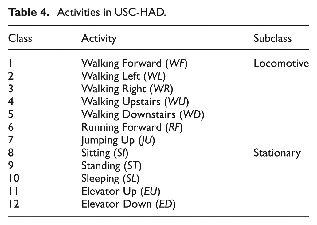
We used one more data set for experiments, called USC-HAD.⁴¹ This data set is composed of raw accelerometer and gyroscope values gathered from a device called MotionNode worn by seven males and seven females. The subjects performed 12 activities for each five times with sampling rate 100 Hz. For each class, we select seven activities for locomotive and other five activities for stationary. Table 4 shows detailed activities.

Table 4.

Activities in USC-HAD.

Class	Activity	Subclass
1	Walking Forward (WF)	Locomotive
2	Walking Left (WL)
3	Walking Right (WR)
4	Walking Upstairs (WU)
5	Walking Downstairs (WD)
6	Running Forward (RF)
7	Jumping Up (JU)
8	Sitting (SI)	Stationary
9	Standing (ST)
10	Sleeping (SL)
11	Elevator Up (EU)
12	Elevator Down (ED)

We have processed the data set with co-efficiencies and FFTs, and finally got 104 features in total. Table 5 shows the features obtained after preprocessing. The data set is partitioned into 80% training and 20% test data.

Table 5.

Features of USC-HAD.

Sensor	Sensor values	Attributes per single sensor value	Attributes per single sensor
Accelerometer	X	Mean	Co-relations between all pairs
	Y	Standard deviation
	Z	Energy
Gyrometer	FFT-X	Interquartile range	Signal magnitude area
	FFT-Y	First to fourth co-efficiencies with autoregressive model using Burg method
	FFT-Z

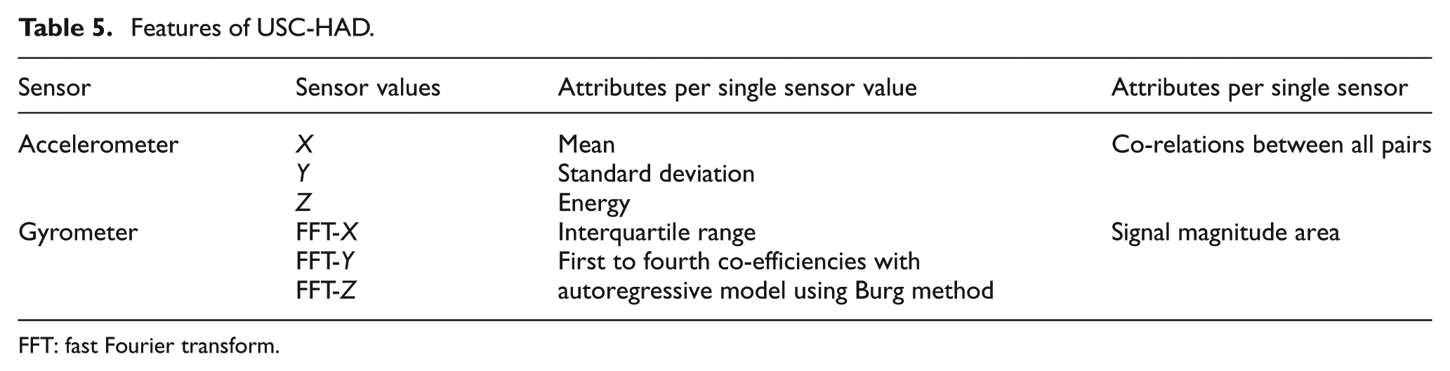
FFT: fast Fourier transform.

As a result of feature extraction using RF VI, first-level CHMM has 63 features and second-level CHMMs for locomotives and stationaries have eight and three features, respectively. Finally, we have obtained TS-CHMM with the highest accuracy of 67.07% as shown in Table 6.

Table 6.

Confusion matrix of the TS-CHMM for USC-HAD.

		Predicted class												Recall (%)
		WF	WL	WR	WU	WD	RF	JU	SI	ST	SL	EU	ED	Recall (%)
Actual class	WF	15	1	0	0	0	3	0	0	0	0	0	0	78.95
	WL	0	14	0	0	0	0	0	0	0	0	0	0	100.00
	WR	0	0	15	2	0	0	0	0	0	0	0	0	88.24
	WU	0	0	8	2	2	0	3	0	0	0	0	0	13.33
	WD	0	6	0	0	2	1	3	0	0	0	0	0	16.67
	RF	2	0	0	0	0	9	1	0	0	0	0	0	75.00
	JU	1	0	0	0	0	7	7	0	0	0	0	0	46.67
	SI	0	0	0	0	0	0	0	13	1	2	0	0	81.25
	ST	0	0	0	0	0	0	0	1	10	0	0	2	76.92
	SL	0	0	0	0	0	0	0	3	0	9	0	0	75.00
	EU	0	0	0	0	0	0	0	0	0	0	0	6	0.00
	ED	0	0	0	0	0	0	0	0	0	0	0	16	100.00
Precision (%)		83.00	67.00	65.00	50.00	50.00	45.00	50.00	76.00	91.00	82.00	0.00	67.00	67.07

WF: Walking Forward; WL: Walking Left; WR: Walking Right; WU: Walking Upstairs; WD: Walking Downstairs; RF: Running Forward; JU: Jumping Up; SI: Sitting; ST: Standing; SL: Sleeping; EU: Elevator Up; ED: Elevator Down.

Figure 10 shows that TS-CHMM has better accuracy than other classification techniques, naïve Bayes, neural network, decision tree, and CHMM in most activities. In the comparison experiment, we adopt CHMM with 12 states per one activity, and neural network with 100 epochs. Table 7 shows the detailed overall accuracies in average and t-test results. TS-CHMM has better accuracy in significance levels compared with all the classification techniques. Compared with the experiments on the first data set, the performance in accuracy has deteriorated significantly. This may show that this data set is more difficult to recognize in terms of the number of activities and the quality of data. However, this does not diminish the superiority of the proposed method compared to the conventional methods in performance.

Figure 10.

TS-CHMM compared to other HAR classifiers (USC-HAD data set).

Table 7.

Fivefold cross validation and t-test result (USC-HAD data set).

	CHMM	NB	NN	DT	TS-CHMM
1	6.51%	58.93%	64.88%	62.50%	64.57%
2	7.79%	54.76%	55.35%	60.12%	62.28%
3	10.71%	53.57%	59.52%	56.96%	65.27%
4	15.45%	60.71%	60.71%	60.71%	63.69%
5	14.91%	58.08%	55.69%	59.28%	61.68%
Avg.	11.07%	57.21%	59.23%	59.91%	63.50%
p-value	0.0000***	0.0081**	0.0159*	0.0198*	–

CHMM: continuous hidden Markov model; NB: naïve Bayes; NN: neural network; DT: decision tree.

Significant at level ***0.001; **0.01; *0.03.

Conclusion

We have shown the benefits of taking advantage of the inherent hierarchical structure of activities using a two-stage system structure in conjunction with CHMMs. This system architecture has also made way to the use of different feature subsets for different subclasses on the second level, as well as to the examination of the effect of varying the BW iterations only, and varying both the number of states and BW iterations for each activity class. We are convinced that more complex activities need to be modeled with more states compared to simpler ones, and CHMMs with less states need more training iterations than CHMMs with more states.

The proposed method is surely to consume some computational resources that might cause the battery consumption, even though it has been implemented to run inside the smartphone due to the powerful hardware of the recent version of smartphones. However, we can think of a couple of plausible solutions to address this issue: (1) offline computation from elsewhere but use the learnt results on-line on the phone, or (2) the computation is achieved on clouds but transmitted to the phone via communication. These solutions might raise some new issues, such as how to adaptively learn and update the results for (1) and how to reduce communication cost for (2).

In addition, we suggest considering a wider range of number of states and iterations while varying them so as to be able to investigate the behavior of CHMMs when used with very large number of states or trained with significantly higher number of iterations. Deriving more effective, energy-efficient features is also another direction for future work.

Footnotes

Academic Editor: Dr Stefano Savazzi

Declaration of conflicting interests

The author(s) declared no potential conflicts of interest with respect to the research, authorship, and/or publication of this article.

Funding

The author(s) disclosed receipt of the following financial support for the research, authorship, and/or publication of this article: This work was supported by the Industrial Strategic Technology Development Program 10044828, Development of Augmenting Multisensory Technology for Enhancing Significant Effects on the Service Industry, funded by the Ministry of Trade, Industry and Energy (MI, Korea).

References

Lara

Labrador

MA.

A survey on human activity recognition using wearable sensors. IEEE Commun Surveys Tutor 2013; 15(3): 1192–1209.

Chen

Hoey

Nugent

. Sensor-based activity recognition. IEEE T Syst Man Cy C 2012; 42(6): 790–808.

Bulling

Blanke

Schiele

A tutorial on human activity recognition using body-worn inertial sensors. ACM Comput Surv 2014; 46(3): 1–33.

Khan

AM.

Recognizing physical activities using Wii remote. Int J Inf Educ Technol 2013; 3(1): 60–62.

Sung

Ponce

Selman

. Unstructured human activity detection from RGBD images. In: Proceedings of the IEEE international conference on robotics and automation, Saint Paul, MN, 14–18 May 2012, pp.842–849. New York: IEEE.

Pei

Guinness

Chen

. Human behavior cognition using smartphone sensors. Sensors 2013; 13(2): 1402–1424.

Anguita

Ghio

Oneto

. A public domain dataset for human activity recognition using smartphones. In: Proceedings of the European symposium on artificial neural networks (ESANN), Bruges, 24–26 April 2013, pp.437–442. ESANN.

Jong

Marchiori

Sebag

. Feature selection in proteomic pattern data with support vector machines. In: Proceedings of the 2004 IEEE symposium on computational intelligence in bioinformatics and computational biology, La Jolla, CA, 7–8 October 2004, pp.41–48. New York: IEEE.

Altun

Barshan

Tunçel

Comparative study on classifying human activities with miniature inertial and magnetic sensors. Pattern Recogn 2010; 43(10): 3605–3620.

10.

Barshan

Yurtman

Investigating inter-subject and inter-activity variations in activity recognition using wearable motion sensors. Comput J 2016; 59(9): 1345–1362.

11.

Chen

Wilcox

Bloomberg

. A comparison of discrete and continuous hidden Markov models for phrase spotting in text images. In: Proceedings of the third international conference on document analysis and recognition, Montreal, QC, Canada, 14–16 August 1995, pp.398–402. New York: IEEE.

12.

Natarajan

Nevatia

Hierarchical multi-channel hidden semi Markov models. In: Proceedings of the international joint conference on artificial intelligence, Hyderabad, India, 6–12 January 2007, pp.2562–2567. AAAI Press.

13.

Bao

Intille

Activity recognition from user-annotated acceleration data. In: Proceedings of the international conference on pervasive computing, Vienna, 18–23 April 2004, pp.1–17. Springer.

14.

Gao

Bourke

Nelson

Evaluation of accelerometer based multi-sensor versus single-sensor activity recognition systems. Med Eng Phys 2014; 36(6): 779–785.

15.

Cleland

Kikhia

Nugent

. Optimal placement of accelerometers for the detection of everyday activities. Sensors 2013; 13: 9183–9200.

16.

Parkka

Ermes

Korpipaa

. Activity classification using realistic data from wearable sensors. IEEE T Inf Technol B 2006; 10(1): 119–128.

17.

Gao

Bourke

Nelson

. A comparison of classifiers for activity recognition using multiple accelerometer-based sensors. In: Proceedings of the IEEE 11th international conference on cybernetic intelligent systems, Limerick, Ireland, 23–24 August 2012, pp.149–153. New York: IEEE.

18.

Chernbumroong

Atkins

Activity classification using a single wrist-worn accelerometer. In: Proceedings of the IEEE international conference on software, knowledge, information management and applications, Benevento, 8–11 September 2011, pp.1–6. New York: IEEE.

19.

Gupta

Dallas

Feature selection and activity recognition system using a single triaxial accelerometer. IEEE Trans Biomed Eng 2014; 61: 1780–1786.

20.

Sharma

Lee

Y-D

Chung

W-Y.

High accuracy human activity monitoring using neural network. In: Proceedings of the third international conference on convergence and hybrid information technology, Busan, South Korea, 11–13 November 2008, pp.430–435. New York: IEEE.

21.

Rubaiyeat

Kim

T-S

Hasan

. Real-time recognition of daily human activities using a single tri-axial accelerometer. In: Proceedings of the 5th international conference on embedded and multimedia computing, Cebu, Philippines, 11–13 August 2010, pp.1–5. New York: IEEE.

22.

Yang

. Toward physical activity diary: motion recognition using simple acceleration features with mobile phones. In: Proceedings of the 1st international workshop on interactive multimedia for consumer electronics, Beijing, China, 19–24 October 2009, pp.1–10. New York: ACM.

23.

Kwapisz

Weiss

Moore

Activity recognition using cell phone accelerometers. ACM SIGKDD Explor Newsl 2010; 12(2): 74–82.

24.

Rabiner

LR.

A tutorial on hidden Markov models and selected applications in speech recognition. P IEEE 1989; 77(2): 257–286.

25.

Archer

Kimes

Empirical characterization of random forest variable importance measures. Comput Stat Data An 2008; 52(4): 2249–2260.

26.

Olguin

Pentland

. Human activity recognition: accuracy across common locations for wearable sensors. In: Proceedings of the international symposium on wearable computers, Montreux, 11–14 October 2006, pp.11–13. New York: IEEE.

27.

Travelsi

Mohammed

Chamroukhi

. An unsupervised approach for automatic activity recognition based on hidden Markov model regression. IEEE Trans Autom Sci Eng 2013; 10(3): 829–835.

28.

Mannini

Sabatini

Machine learning methods for classifying human physical activity from on-body accelerometers. Sensors 2010; 10: 1154–1175.

29.

Khan

Lee

Y-K

Lee

S-Y

. A triaxial accelerometer-based physical-activity recognition via augmented-signal features and a hierarchical recognizer. IEEE T Inf Technol B 2010; 14(5): 1166–1172.

30.

Lee

Y-S

Cho

S-B

. Activity recognition using hierarchical hidden Markov models on a smartphone with 3D accelerometer. In: Proceedings of the international conference on hybrid intelligent systems, Wroclaw, 23–25 May 2011, pp.460–467. Berlin: Springer.

31.

Luktarhan

Jia

. Multi-stage attack detection algorithm based on hidden Markov model. In: Proceedings of the international conference on web information systems and mining, Chengdu, China, 26–28 October 2012, pp.275–282. New York: ACM.

32.

Lee

D-H

Kim

D-Y

Jung

J-I.

Multi-stage intrusion detection system using hidden Markov model algorithm. In: Proceedings of the international conference on information science and security, Seoul, South Korea, 10–11 January 2008, pp.72–77. New York: IEEE.

33.

Nguyen-Duc-Thanh

Lee

S-Y

Kim

D-H.

Two-stage hidden Markov model in gesture recognition for human robot interaction. Int J Adv Robot Syst 2012; 9(39): 1–10.

34.

Ronao

Cho

S-B.

Human activity recognition using smartphone sensors with two-stage continuous hidden Markov models. In: Proceedings of the international conference on natural computation, Xiamen, China, 19–21 August 2014, pp.681–686. New York: IEEE.

35.

Breiman

Random forests. Mach Learn 2001; 45(1): 5–32.

36.

Genuer

Poggi

Tuleau-Malot

Variable selection using random forests. Pattern Recogn Lett 2010; 31(14): 2225–2236.

37.

Yan

Subbaraju

Chakraborty

. Energy-efficient continuous activity recognition on mobile phones: an activity-adaptive approach. In: Proceedings of the international symposium on wearable computers, Newcastle upon Tyne, 18–22 June 2012, pp.17–24. New York: IEEE.

38.

Becker

Chambers

Wilks

AR.

The new S. language. Pacific Grove, CA: Wadsworth & Brooks/Cole, 1988.

39.

Jolliffe

Principal component analysis. Hoboken, NJ: John Wiley & Sons, 2002.

40.

Venables

Ripley

BD.

Modern applied statistics with S. 4th ed.New York: Springer, 2002.

41.

Zhang

Sawchuk

. USC-HAD: a daily activity dataset for ubiquitous activity recognition using wearable sensors. In: Proceedings of the ACM international conference on ubiquitous computing (UbiComp), Pittsburgh, PA, 5–8 September 2012, pp.1036–1043. New York: ACM.