Sage Journals: Discover world-class research

Abstract

Lithium-ion battery has been widely used in various fields due to its excellent performance. How to accurately predict its current capacity throughout a battery full lifetime has been a key technology for power system management, assurance, and predictive maintenance. In order to overcome low precision problem in long-term prediction for lithium-ion battery capacity, this article proposes a multi-scale fusion prediction method based on ensemble empirical mode decomposition and nonlinear autoregressive models neural networks. The proposed method uses ensemble empirical mode decomposition to decompose the battery capacity measurement sequence to generate multiple intrinsic mode function components on different scales. Then, each component is predicted by nonlinear autoregressive neural networks; finally, the prediction results of each component are reconstructed to obtain the final battery capacity prediction sequence. Experimental results show that the proposed method has higher prediction accuracy and signal adaptability than single nonlinear autoregressive neural networks.

Keywords

Lithium-ion battery capacity prediction ensemble empirical mode decomposition autoregressive models neural networks

Introduction

Lithium-ion batteries, as an energy source for many complex electronic systems, play an important role in the functional capabilities of electronic systems. Many investigations show that power system degradation is the main cause of system fault or failure.¹ Thus, the life health status of power source directly affects the safety and reliability of a hybrid power system.² In this case, an effective technique to monitor battery status can greatly improve power system reliability. For lithium-ion battery, remaining useful life (RUL) prediction has become a hot research subject.³ Several research works of RUL prediction can be founded, such as the world’s leading University of Maryland Advanced Life Week Engineering Center^4,5 and NASA’s Prognostics Center of Excellence (PCoE).

In general, RUL prediction methods mainly include model-based and data-driven methods. These two methods have been widely used in prognostic of batteries and fuel cells.⁶ Model-based methods describe battery internal aging mechanism. For example, the battery aging mechanism model studies the influence of several aging factors such as the state of charge, electrolyte concentration, and diffusion coefficient on the state variables.^7,8

Thomas et al. present an alternative framework based on a degradation model; this model focuses on degradation rate. This framework facilitates the prediction of cell life when the stress level is dynamic.⁹ Lee et al.¹⁰ produce a physics-based one-dimensional model of a lithium-ion cell, in order to estimate battery status based on discrete-time realization algorithm.

For the estimation algorithm in model-based method, several approaches can be founded, such as Kalman filtering,¹¹ unscented Kalman filtering (UKF),¹² and particle filtering (PF).¹³ These filter-based methods can provide acceptable prediction results. The precondition for the application of the filtering method is to accurately establish the degradation model of the battery. In practical applications, it is difficult to accurately describe the true performance degradation state of the lithium-ion battery.

The data-driven method is based on historical data of a lithium-ion battery and does not require an in-depth understanding of the internal aging mechanism of the battery. Thus, the data-driven methods have received widespread attention, such as autoregressive moving average (ARMA) model, support vector regression (SVR), and artificial neural networks.¹⁴

In terms of RUL prediction of lithium-ion batteries, the AR model describes the future performance state as a combination of linear equations and random errors based on historical state observations. The advantages of the AR are simple calculation and low complexity.^13,15,16 However, the main disadvantages are inaccuracy for the long-term prediction.

SVR is another advanced tool for prediction. S Wang et al.¹⁷ devised a non-iterative prediction model based on flexible support vector regression (F-SVR) and an iterative multi-step prediction model, where the energy efficiency and battery working temperature are considered as input physical characteristics. T Qin et al. employed SVR into battery state of health (SOH) prognostics. The proposed particle swarm optimization (PSO)–SVR model can be used for long-term prediction and can obtain acceptable SOH prediction results.¹⁸ However, the SVR has some shortcomings: the kernel function must satisfy the Mercer condition; the sparsity is limited, and the number of support vectors is sensitive to the error boundary.

Artificial neural networks (ANNs) are a data-based, typical nonlinear approach with self-organization and self-learning capabilities. For the RUL prediction of lithium-ion battery, the battery aging nonlinear can be well trained and predicted by neural networks. The National Center for Electronics Manufacturing Excellence of USA has applied neural networks to RUL prediction of batteries. In order to improve the stability of prediction, the prediction values of neural networks, fuzzy logic, and ARMA models are further integrated.¹⁹ Parthiban et al.²⁰ used the artificial neural networks to predict the life decay of lithium-ion batteries. The input of the neural networks is the number of cycles (battery charge and discharge cycle), and the output is the capacity of the battery. The trained neural networks have a good consistency between the predicted results and the regression results of the training data.²¹ In recent years, some deep learning approach has been applied into battery RUL prediction. The long short-term memory (LSTM) recurrent neural networks (RNNs) are employed to learn the long-term dependencies among the degraded capacities of lithium-ion batteries.²² A fusion RUL prediction approach based on deep belief networks (DBNs) and relevance vector machine (RVM) is proposed for lithium-ion battery remaining useful life prediction.²³ However, neural networks have inherent problems, for example, model identification, complex structure, low computational efficiency, and over-learning.

At the same time, hybrid methods are also applied to RUL predictions. For example, Y Zhou and M Huang²⁴ proposed a novel approach which combines empirical mode decomposition (EMD) and autoregressive integrated moving average (ARIMA) model for RUL prognostic. Three metabolic gray models are presented to predict the lithium-ion battery capacity.²⁵ A hybrid prediction model is presented to estimate the RUL of lithium-ion batteries.²⁶

As a critical performance of lithium-ion batteries, capacity represents the available energy stored in the fully charged lithium-ion batteries. It is usually used to analyze the state-of-health (SoH) for batteries. Therefore, this article studies the data-driven lithium-ion battery capacity prediction problem. Because the battery system is a time-varying, highly nonlinear system, it is a challenge to precisely predict the capacity of a battery. The capacity regeneration phenomenon of lithium-ion batteries related to physicochemical aspects, temperature and load conditions during charge and discharge cycles further increase the difficulty of prediction.²⁷ This study found that the raw of battery capacity curve can be considered as a hybrid signal with multi-scale components, where global deterioration and capacity regeneration are supposed to be of different scales.²⁸ Therefore, if the global deterioration and capacity regeneration parts can be decomposed from capacity signal and then separately predicted, it will help to improve the prediction accuracy. In this article, inspired by fusion approach,²⁹ we propose a multi-scale fusion prediction method based on ensemble empirical mode decomposition (EEMD) and nonlinear autoregressive (NAR) neural networks. First, EEMD is used to decouple the global deterioration trend and capacity regeneration from the raw capacity curve. Then we employ NAR neural networks to establish the nonlinear prediction models for each of decomposition components. Finally, all the predicted components are merged to obtain the final comprehensive capacity prediction. In addition, the capacity prediction results obtained by EEMD + NAR are compared with single NAR to demonstrate the performance of our proposed prediction method.

The rest of the paper is organized in the following order: The theory of EEMD and NAR neural networks are introduced in section “Related algorithms.” Section “Multi-scale fusion prediction method” proposes the multi-scale fusion prediction method. Section “Prediction result and discussion” presents the prediction results and gives discussion. Finally, conclusion is drawn in section “Conclusion.”

Related algorithms

EEMD method

Although EMD is self-adaptation and very suitable for nonlinear and non-stationary signals, its modal aliasing influences the correctness and accuracy of the analysis results and thus reduces the effectiveness of signal decomposition. To address the EMD modal aliasing problem, ZH Wu and NE Huang³⁰ proposed the improved EEMD method. The EEMD method is inspired by the method of averaging multiple measurements of a component in statistics, in order to improve the accuracy of the measurement. EEMD first adds multiple sets of different white noise sequences into the source signal, then separately performs EMD decomposition in order to obtain intrinsic mode function (IMF) components of each noise-containing signal, and averages each group of IMF components of EEMD. The addition of white noise guarantees continuity in the time domain of each modal function and thus reduces modal aliasing. The main steps of EEMD are as follows:

1. External initialization, adding a group of zero mean and equal variance random white noise sequence into the original signal $x_{0} (t)$ , a group of signals ${x_{1} (t), x_{2} (t), \dots, x_{m} (t)}$ consisting of $m$ noise-added signal is established.

If a set of white noise signals is ${n_{1} (t), n_{2} (t), \dots, n_{m} (t)}$ , then the group of signals can be obtained by

{\begin{matrix} x_{1} (t) = x_{0} (t) + n_{1} (t) \\ x_{2} (t) = x_{0} (t) + n_{2} (t) \\ ⋮ \\ x_{m} (t) = x_{0} (t) + n_{m} (t) \end{matrix}

(1)

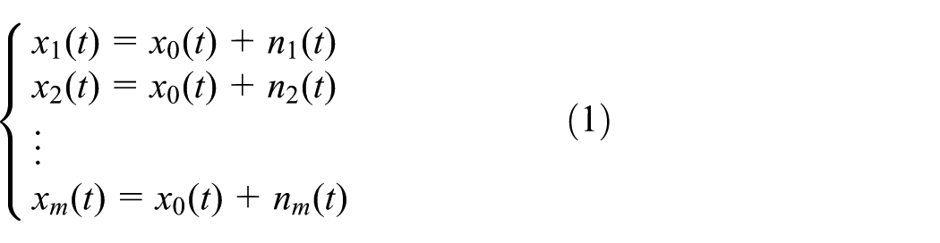
2. Perform EMD decomposition of the signals in the signal collection after adding noise. The EMD decomposition results are

{[\begin{matrix} c_{i 1} (x, y) & c_{i 2} (x, y) & \dots & \dots & c_{iN} (x, y) \end{matrix}], Re s_{iN} (x, y)}

(2)

where $c_{ij} (x, y)$ is the jth IMF component of the ith signal in the decomposed signal collection; $N$ is the number of decomposed IMF component; $Re s_{iN} (x, y)$ is the final residual component.

3. Repeat the above steps for each signal $x_{i}$ in the collection and perform EMD decomposition separately. Get $m$ group IMF components ${[c_{11} c_{12} c_{13} \dots c_{1 N}], \dots [c_{m 1} c_{m 2} c_{m 3} \dots c_{m N}]}$ and m sets of residue $[{Res}_{1 N} {Res}_{2 N} {Res}_{3 N} \dots {Res}_{m N}]$ .

4. Calculation the mean of the $m$ group IMF components $[\begin{matrix} C_{E 1} & C_{E 2} & C_{E 3} & \dots & C_{EN} \end{matrix}]$ and $m$ group residue $Re s_{EN}$ based on the following equation

C_{Ej} = \frac{1}{m} \sum_{i = 1}^{m} c_{ij}, j = 1, 2, \dots, N, Re s_{EN} = \frac{1}{m} \sum_{i = 1}^{m} Re s_{iN}

(3)

Then the inverse transformed signal $x_{E}$ can be represented as

x_{E} (t) = \sum_{j = 1}^{N} C_{Ej} (t) + Re s_{EN} (t)

(4)

In this process, since the white noise has a random characteristic with a mean of zero and equal variance, the overall average of each EMD decomposition is taken as the final decomposition result of the EEMD decomposition IMF components, in order to eliminate the influence of the white noise. The added white noise guarantees the continuity of each modal function in the time domain, thus reducing modal aliasing and endpoint effects. The IMFs decomposition is a process that decomposes the minimum scale to the maximum. It extracts the detail information of the signal in different frequency domains. This is similar to the wavelet decomposition process. However, if wavelets are selected from different wavelet basis function, the decomposition results are totally different. This is the reason why we use EEMD method, as there is no basis functions in EEMD decomposition process.

NAR neural networks

The NAR neural networks have feedback and memory functions. The output of each moment is based on the dynamic synthesis result of the system before the current time.³¹ It has significant advantages in modeling and simulation of time series dynamic changes.³¹

Typical NAR neural networks are mainly composed of input layer, hidden layer, output layer, and input delay function. The basic structure is shown in Figure 1.

Figure 1.

Standard NAR schematic structure of the neural networks.

In Figure 1, $y (t)$ is the output of the neural networks, $1 : 2$ represents the delay order, $W$ is the joint weight, and $b$ is the threshold of NAR neural networks. The NAR neural networks model can be expressed as

y (t) = f (y (t - 1), y (t - 2), \dots, y (t - d))

(5)

where $d$ is delay order and $f (\cdot)$ is neural networks model. It can be seen from the equation that the value of $y (t)$ is determined by the values of $y (t - 1), y (t - 2), \dots, y (t - d)$ , which indicates that based on the continuity of data development, the model uses past values to estimate the current value.

The prediction method of the NAR model adopts the recursive prediction method. The main purpose of this prediction method is to recycle the forward prediction value of one step. The basic idea is

y (t_{n}) = f (y (t_{n} - 1), y (t_{n} - 2), \dots, y (t_{n} - d))

(6)

When $k = 1$ , the first-step prediction value $y (t_{n})$ can be obtained. When predicting $y (t_{n} + 1)$ , a new sample can be formed by adding the one-step predicted value $y (t_{n})$ into the original sample

(y (t_{n} - d), \dots, y (t_{n} - 2), y (t_{n} - 1), y (t_{n}))

(7)

Then the second-step prediction results $y (t_{n} + 1)$ can be calculated. Then, the new sample is constructed

(y (t_{n} - d), \dots, y (t_{n} - 2), y (t_{n} - 1), y (t_{n}), y (t_{n} + 1))

(8)

The three-step prediction value is obtained through the NAR networks, and the loop is continued until the required k-step prediction value is obtained.

Multi-scale fusion prediction method

Experiment data analysis

In this article, the test data set was chosen from NASA Ames Prognostics Center.^32,33 The battery test bench contains an environmental chamber, chargers, loads, battery impedance tester, a suite of sensors, some custom switching relay circuitries, data acquisition cards, and a computer or a DSP (digital signal processor) chip for control and analysis. The lithium-ion batteries were run through three different operational steps: charge, discharge, and impedance. The operation process is as follows:

Charge: charging was first conducted at constant current (CC) 1.5 A until the charge voltage reached the top cutoff voltage (set as 4.2 V). Then, charging was turned into constant voltage (CV) mode until the charging current dropped below 20 mA.

Discharge: discharging was performed from 4.2 V to a predefined cutoff voltage. The end-of-life criterion is defined as a 30% fade in rated capacity (1.4 Ah).

Impedance measurement: measurement was performed through an electrochemical impedance spectroscopy frequency sweeping from 0.1 to 5 kHz.

We use the data of batteries No.6, No.7 to demonstrate the performance of our proposed approach for battery capacity prediction. We can get battery capacity curves as shown in Figure 2. We can see that there is an obviously descent trend, the global deterioration, and a lot of capacity regenerations.

Figure 2.

Capacity curves of Battery No.6 and No.7.

In order to demonstrate the effectiveness of EEMD, we present the decomposition result of battery No.6 and No.7. In EEMD algorithm, the IMF number is set to 3, the ensemble number for EEMD is set to 10, and the ratio of the standard deviation of the added noise and that of the original signal are set to 0.01.

As we can see Figures 3 –6, there are three IMFs (i.e. IMF 1, IMF 2, IMF 3) and residue. Both IMF 1 and IMF 2 have high frequency fluctuations which correspondingly reflect the high-frequency capacity regenerations. IMF 3 has relatively low frequency fluctuations. In general, IMF 1, IMF 2, and IMF 3 together show the capacity regeneration phenomenon of lithium-ion battery. Thus, we can use the IMFs to describe the capacity regeneration phenomenon. The residues are plotted on Figures 3 and 5 with raw battery capacity data series. Pearson correlation analysis³⁴ can be applied to quantitatively verify the linear relationship between the raw SOH series and the derived residue. The calculation results are summarized in Table 1. From Table 1, Pearson correlation coefficient and root mean squared error (RMSE) between them of battery No.6 is 0.995 and 0.019. Pearson correlation coefficient and RMSE between them of battery No.7 is 0.9975 and 0.0082, respectively, indicating that the residue is accurate enough to describe the battery deterioration trend. Therefore, the residues are reasonable enough to describe the global deterioration of lithium-ion batteries. In another aspect, we can conclude EEMD is effective in decomposing the battery capacity series.

Figure 3.

No.6 battery capacity curve and residue curve of EEMD decomposition.

Figure 4.

No.6 battery capacity IMF curves of EEMD decomposition.

Figure 5.

No.7 battery capacity curve and residue curve of EEMD decomposition.

Figure 6.

No.7 battery capacity IMF curves of EEMD decomposition.

Table 1.

The linear relationship analysis results between the raw SOH series and the derived residue of EEMD.

Battery No.	Pearson correlation coefficient	RMSE
B0006	0.995	0.019
B0007	0.9975	0.0082

SOH: state of health; EEMD: ensemble empirical mode decomposition; RMSE: root mean squared error.

Proposed prediction method

It can be seen from the above decomposition results that the global deterioration and capacity regeneration curves differ greatly in frequency characteristics and shapes. If the prediction is directly performed, it is difficult to adapt to both characteristics at the same time. Therefore, we are drawing on the idea of multi-scale decomposition and data fusion in image fusion, proposed multi-scale fusion prediction method for battery capacity. The detailed prediction method steps for battery capacity are shown in Figure 7. The steps of multi-scale fusion prediction method based on EEMD and NAR neural networks are as follows:

Load the raw battery capacity series;

Perform EEMD to decouple raw battery capacity series into a number of battery capacity decomposition components which contain global deterioration trend {Residue} and capacity regeneration {IMFs};

First, separate the decoupled IMFs and residue data into training data and prediction test data. Then NAR neural networks for each decomposition components are designed and trained. Next, we make predictions for each decomposition components with NAR neural networks.

Fusion all the separate prediction results to get the comprehensive battery capacity prediction.

Figure 7.

Multi-scale fusion prediction procedure of battery capacity.

Prediction result and discussion

In this section, the predicted performance qualities of NAR neural networks direct prediction method and proposed method are investigated by applying them to predict the capacity over the lifetime of a battery. We use the same structure of the networks in both prediction methods.

Evaluation criteria

Before the battery capacity prediction verification, we define the absolute error (AE), mean absolute percentage error (MAPE), and RMSE as the main evaluation criteria to evaluate the prediction performance, and they are shown as follows:

1. AE

AE (t) = | y (t) - y_{p} (t) |

(9)

where $y (t)$ is battery capacity raw data sequence and $y_{p} (t)$ is prediction result sequence.

2. MAPE

MAPE = \frac{1}{M} \sum_{i = 1}^{M} \frac{| y (i + n_{s}) - y_{p} (i + n_{s}) |}{y (i + n_{s})}

(10)

where $y (t)$ is battery capacity raw data sequence, $y_{p} (t)$ is prediction result sequence, $M$ is the number of predicted data, and $n_{s}$ is the prediction starting cycle number.

3. RMSE

RMSE = \sqrt{\frac{1}{M} \sum_{i = 1}^{M} {[y (i + n_{s}) - y_{p} (i + n_{s})]}^{2}}

(11)

Prediction result

Here, we design two test cases. In case 1, 70% of the raw data is trained using NAR neural networks, and then the remaining 30% is used for prediction performance verification. The data are shown in Figures 8 and 9.

Figure 8.

Data configure of No.6 battery in case 1.

Figure 9.

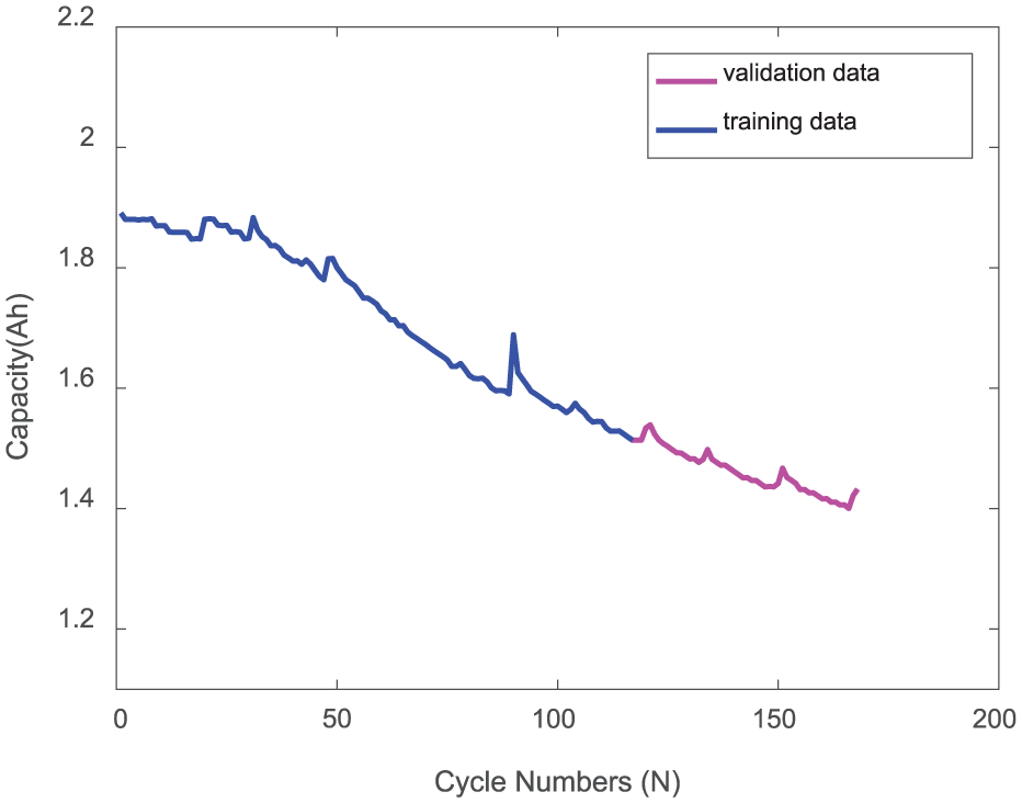
Data configure of No.7 battery in case 1.

The NAR neural networks are designed as the numbers of hidden layer are 2. The neural cell numbers of hidden layer are 6 and 3 respectively. The delay number of input is 5. The structure of NAR networks is shown as Figure 10.

Figure 10.

The structure of NAR networks in case 1.

We first repeat 30 battery capacity predictions for each battery using NAR neural networks with raw data series and select the best prediction result. Second, the proposed method is also repeated 30 battery capacity predictions and selects the best prediction result. The prediction results are shown in Figures 11 –20 and Table 2.

Figure 11.

Comparison of prediction results for No.6 battery in case 1.

Figure 12.

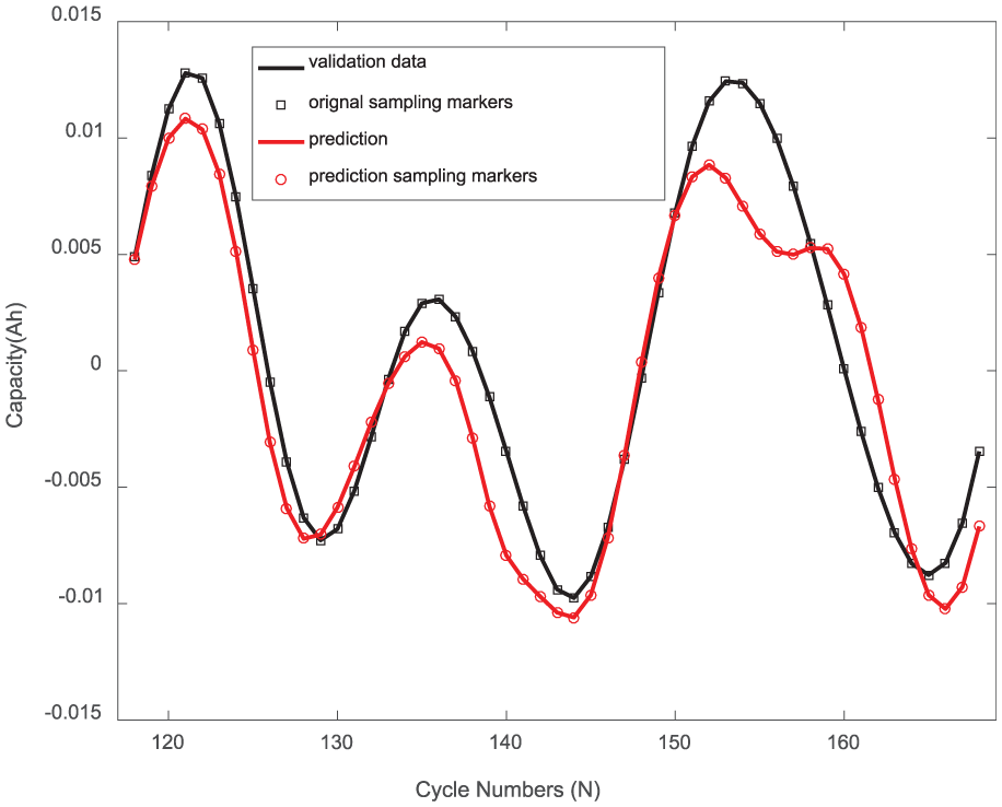
Prediction results of proposed method for IMF1 of No.6 battery.

Figure 13.

Prediction results of EEMD + NAR method for IMF2 of No.6 battery.

Figure 14.

Prediction results of EEMD + NAR method for IMF3 of No.6 battery in case 1.

Figure 15.

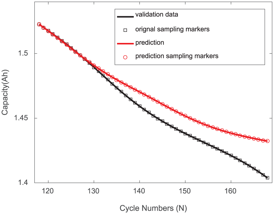
Prediction results of EEMD + NAR method for residue of No.6 battery.

Figure 16.

Comparison of prediction results for No.7 battery in case 1.

Figure 17.

Prediction results of EEMD + NAR method for IMF1 of No.7 battery.

Figure 18.

Prediction results of EEMD + NAR method for IMF2 of No.7 battery.

Figure 19.

Prediction results of EEMD + NAR method for IMF3 of No.7 battery in case 1.

Figure 20.

Prediction results of EEMD + NAR method for residue of No.7 battery.

Table 2.

The prediction results in case 1.

Battery No.	Method	Max AE	MAPE	RMSE
B0006	NAR	0.0682	0.0151	0.0245
	EEMD + NAR	0.0499	0.0097	0.016
	Performance improvement	26.8%	35.7%	34.6%
B0007	NAR	0.0529	0.0129	0.0235
	EEMD + NAR	0.04	0.0081	0.0157
	Performance improvement	24.3%	37.2%	33.1%

AE: absolute error; MAPE: mean absolute percentage error; RMSE: root mean squared error; NAR: nonlinear autoregressive; EEMD: ensemble empirical mode decomposition.

Bold values highlight the extent of performance improvement.

From Table 2, we can see that all the verification indicators of NAR are bigger than the proposed EEMD + NAR method. For No.6 battery, the values of maximum AE, MAPE, and RMSE with EEMD + NAR are 0.0499, 0.0097, and 0.016, respectively, while the NAR values are 0.0682, 0.0151, and 0.0245, respectively, in case 1. The prediction performance of AE, MAPE, and RMSE are increased by 26.8%, 35.7%, and 34.6%, respectively, using EEMD + NAR method. For No.7 battery, we can also find the maximum AE, MAPE, RMSE with EEMD + NAR are 0.04, 0.0081, and 0.0157, respectively, while the values with NAR are 0.0529, 0.0129, and 0.0235, respectively, in case 1. The prediction performances of AE, MAPE, and RMSE are improved by 24.3%, 37.2%, and 33.1%, respectively, using EEMD + NAR method.

In case 2, 40% of the raw data is trained using dynamic neural networks, and then the remaining 60% is used for prediction performance verification. The data configure is shown in Figures 21 and 22.

Figure 21.

Data configure of No.6 battery in case 2.

Figure 22.

Data configure of No.7 battery in case 2.

The NAR neural networks are designed as the numbers of hidden layer are 2. The neural cell numbers of hidden layer are 50 and 20 respectively. The delay number of input is 20. The structure of NAR networks is shown in Figure 23.

Figure 23.

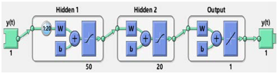
The structure of NAR networks in case 2.

Figure 24.

Comparison of prediction results for No.6 battery in case 2.

Figure 25.

Prediction results of EEMD + NAR method for IMF1 of No.6 battery.

Figure 26.

Prediction results of EEMD + NAR method for IMF2 of No.6 battery.

Figure 27.

Prediction results of EEMD + NAR method for IMF3 of No.6 battery in case 2.

Figure 28.

Prediction results of EEMD + NAR method for residue of No.6 battery.

Figure 29.

Comparison of prediction results for No.7 battery in case 2.

Figure 30.

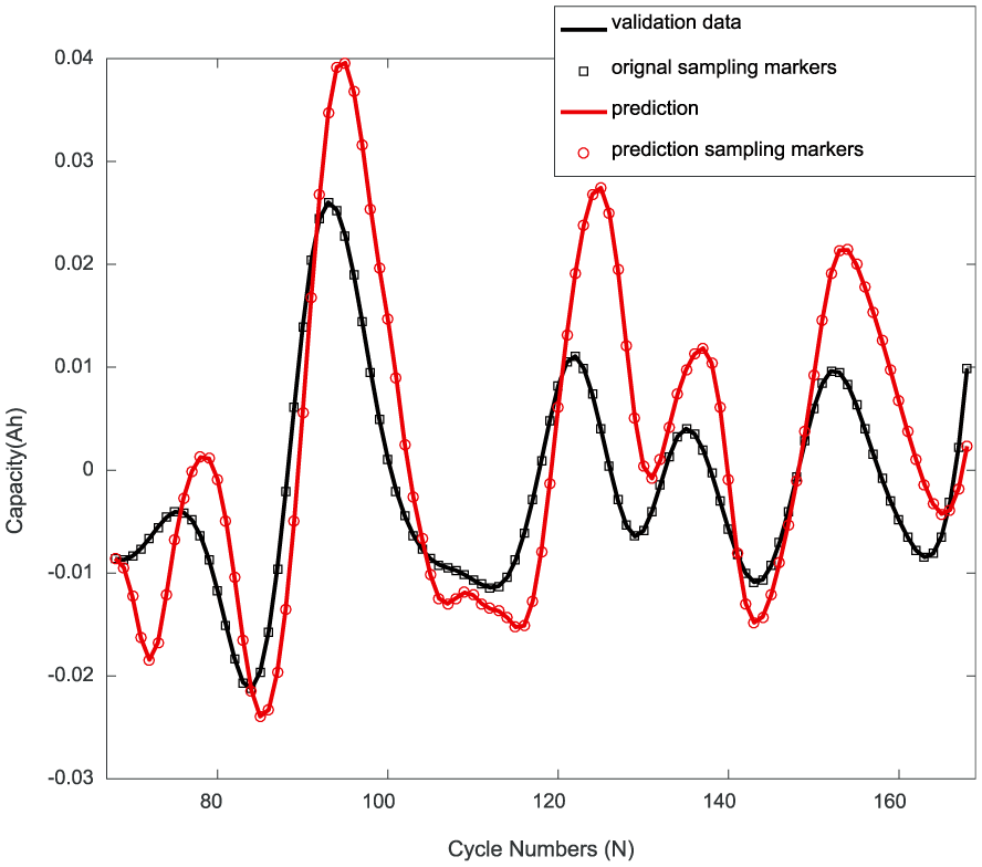
Prediction results of EEMD + NAR method for IMF1 of No.7 battery.

Figure 31.

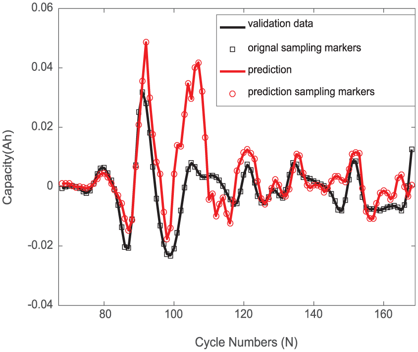
Prediction results of EEMD + NAR method for IMF2 of No.7 battery.

Figure 32.

Prediction results of EEMD + NAR method for IMF3 of No.7 battery in case 2.

Figure 33.

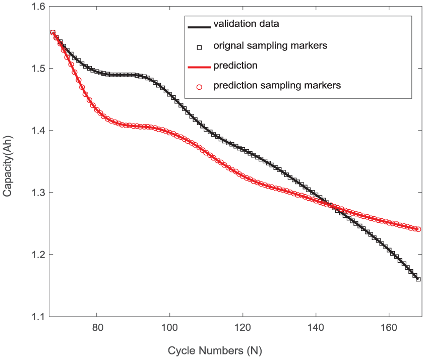
Prediction results of EEMD + NAR method for residue of No.7 battery.

Table 3.

The prediction results in case 2.

Battery No.	Method	Max AE	MAPE	RMSE
B0006	NAR	0.233	0.045	0.0802
	EEMD + NAR	0.174	0.0312	0.052
	Performance improvement	25.3%	30.6%	35.1%
B0007	NAR	0.1746	0.0480	0.0880
	EEMD + NAR	0.157	0.0263	0.0483
	Performance improvement	10.1%	45.2%	45.1%

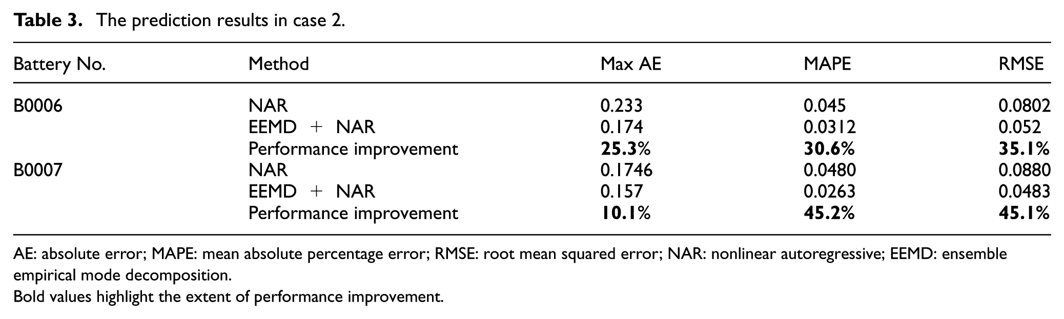
AE: absolute error; MAPE: mean absolute percentage error; RMSE: root mean squared error; NAR: nonlinear autoregressive; EEMD: ensemble empirical mode decomposition.

Bold values highlight the extent of performance improvement.

From Table 3, we can see that all the verification indicators of NAR networks are bigger than that with EEMD + NAR. For No.6 battery, the values of maximum AE, MAPE, and RMSE with EEMD + NAR are 0.174, 0.0312, and 0.052, respectively, while the NAR values are 0.233, 0.045, and 0.0802, respectively, in case 2. The prediction performances of AE, MAPE, and RMSE are increased by 25.3%, 30.6%, and 35.1%, respectively, using EEMD + NAR method. For No.7 battery, we can also find the maximum AE, MAPE, RMSE with EEMD-NAR are 0.157, 0.0263, and 0.0483, respectively, while the values with NAR are 0.1746, 0.048, and 0.088, respectively, in case 2. The prediction performances of AE, MAPE, and RMSE are increased by 10.1%, 45.2%, and 45.1%, respectively, using EEMD + NAR method.

Result discussion

From Tables 2 and 3, the results show that EEMD significantly improves the precision of battery capacity. All of the predicted results made by EEMD + NAR method are much closer to the true value than NAR networks method. All of the three indicators are small, which indicates the accuracy of the battery capacity prediction. The predicted performance improvement is 10% minimum and the maximum is 45%. Therefore, it is reasonable to draw the conclusion that the proposed EEMD + NAR method has prominent performance with high accuracy and effectiveness, and it also is able to provide an accurate battery parameters prediction assisting in RUL prognostic.

Conclusion

The main contributions of this article can be summarized as follows:

Global deterioration trend and capacity regeneration are extracted from raw battery series by EEMD without losing the characteristic of raw data series. After decomposition, Pearson correlation coefficient and RMSE between them of battery No.6 are 0.995 and 0.019. The Pearson correlation coefficient and RMSE of battery No.6 are 0.9975 and 0.0082. This can be concluded that the residue is accurate enough to describe the battery deterioration trend.

The proposed method improves the battery capacity prediction accuracy of NAR methods by 30%–45% in RMSE indicator.

According to the above two points and the analyses in section “Prediction result and discussion,” we can conclude that our proposed method is effective and accurate in battery capacity prediction. Although EEMD + NAR method gets a better prediction performance than NAR method, as the prediction length increases, the prediction effect of NAR neural networks on the global deterioration trend signal gradually deteriorates. In the future, we will focus more on the global deterioration trend signal prediction with other methods, for example, gray model or ARMA model, in order to improve the accuracy of the prediction performance.

Footnotes

Handling Editor: Daming Zhou

Declaration of conflicting interests

The author(s) declared no potential conflicts of interest with respect to the research, authorship, and/or publication of this article.

Funding

The author(s) disclosed receipt of the following financial support for the research, authorship, and/or publication of this article: This work was supported by the Joint Fund for Advanced Equipment Research and Aerospace Science and Technology of China (Grant No. 6141B06220220301).

ORCID iD

Pei Wang

References

Shea

JJ.

Spacecraft power technologies. IEEE Electr Insul Mag 2002; 18(3): 59–60.

Zhou

Al-Durra

Matraji

et al . Online energy management strategy of fuel cell hybrid electric vehicles: a fractional-order extremum seeking method. IEEE T Ind Electron 2018; 65(8): 6787–6799.

Rezvanizaniani

Liu

Chen

et al . Review and recent advances in battery health monitoring and prognostics technologies for electric vehicle (EV) safety and mobility. J Power Sources 2014; 256(12): 110–124.

Xing

Pecht

et al . State of charge estimation of lithium-ion batteries using the open-circuit voltage at various ambient temperatures. Appl Energ 2014; 113(1): 106–115.

Williard

Chen

et al . State of charge estimation for electric vehicle batteries using unscented Kalman filtering. Microelectron Reliab 2013; 53(6): 840–847.

Zhou

Nguyen

Breaz

et al . Global parameters sensitivity analysis and development of a two-dimensional real-time model of proton-exchange-membrane fuel cells. Energ Convers Manage 2018; 162: 276–292.

Celaya

Kulkarni

Saha

et al . Accelerated aging in electrolytic capacitors for prognostics. In: Proceedings of the annual reliability and maintainability symposium, Reno, NV, 23–26 June 2012, pp.1–6. New York: IEEE.

Oudalov

Ulbig

et al . Modeling of lithium-ion battery degradation for cell life assessment. IEEE T Smart Grid 2018; 9(2): 1131–1140.

Thomas

Bloom

Christophersen

et al . Rate-based degradation modeling of lithium-ion cells. J Power Sources 2012; 206: 378–382.

10.

Lee

Chemistruck

Plett

GL.

One-dimensional physics-based reduced-order model of lithium-ion dynamics. J Power Sources 2012; 220: 430–448.

11.

Tang

et al . A remaining useful life prediction approach for lithium-ion batteries using Kalman filter and an improved particle filter. In: Proceedings of the international conference on prognostics and health management, Ottawa, ON, 20–22 June 2016, pp.1–5. New York: IEEE.

12.

Xian

Long

et al . Prognostics of lithium-ion batteries based on the Verhulst model, particle swarm optimization and particle filter. IEEE T Instrum Meas 2014; 63(1): 2–17.

13.

Liu

Luo

Liu

et al . Lithium-ion battery remaining useful life estimation based on fusion nonlinear degradation AR model and RPF algorithm. Neural Comput Appl 2014; 25(3–4): 557–572.

14.

Zhou

Al-Durra

Zhang

et al . Online remaining useful lifetime prediction of proton exchange membrane fuel cells using a novel robust methodology. J Power Sources 2018; 399: 314–328.

15.

Long

Xian

Jiang

et al . An improved autoregressive model by particle swarm optimization for prognostics of lithium-ion batteries. Microelectron Reliab 2013; 53(6): 821–831.

16.

Jiang

Xian

Long

et al . Analysis of data-driven prediction algorithms for lithium-ion batteries remaining useful life. Adv Mater Res 2013; 717: 390–395.

17.

Wang

Zhao

et al . Prognostics of lithium-ion batteries based on battery performance analysis and flexible support vector regression. Energies 2014; 7(10): 6492–6508.

18.

Qin

Zeng

Guo

Robust prognostics for state of health estimation of lithium-ion batteries based on an improved PSO–SVR model. Microelectron Reliab 2015; 55(9–10): 1280–1284.

19.

Shimanek

. Empfasis: a publication of the national electronics manufacturing center of excellence. Navy Mantech Report, January 2003. ACI Technologies Inc.

20.

Parthiban

Ravi

Kalaiselvi

Exploration of artificial neural network [ANN] to predict the electrochemical characteristics of lithium-ion cells. Electrochim Acta 2007; 53(4): 1877–1882.

21.

Liu

Saxena

Goebel

. An adaptive recurrent neural network for remaining useful life prediction of lithium-ion batteries. In: Proceedings of the annual conference of the prognostics and health management society, 28 September 2010, pp.1–9. Portland: PHM Society.

22.

Zhang

Xiong

et al . Long short-term memory recurrent neural network for remaining useful life prediction of lithium-ion batteries. IEEE T Veh Technol 2018; 67(7): 5695–5705.

23.

Zhao

Zhang

Liu

et al . Lithium-ion battery remaining useful life prediction with deep belief network and relevance vector machine. In: Proceedings of the international conference on prognostics and health management, Dallas, TX, 19–21 June 2017, pp.7–13. New York: IEEE.

24.

Zhou

Huang

Lithium-ion batteries remaining useful life prediction based on a mixture of empirical mode decomposition and ARIMA model. Microelectron Reliab 2016; 65: 265–273.

25.

Chen

Lin

et al . Prediction of lithium-ion battery capacity with metabolic grey model. Energy 2016; 106: 662–672.

26.

Zhang

Yuan

et al . Prognostics of lithium-ion batteries based on wavelet denoising and DE-RVM. Comput Intell Neurosci 2015; 2015(1): 918305.

27.

Olivares

Cerda Munoz

Orchard

et al . Particle-filtering-based prognosis framework for energy storage devices with a statistical characterization of state-of-health regeneration phenomena. IEEE T Instrum Meas 2013; 62(2): 364–376.

28.

Shen

et al . State of health estimation of lithium-ion batteries: a multiscale Gaussian process regression modeling approach. AIChE J 2015; 61(5): 1589–1600.

29.

Zhou

Al-Durra

Gao

et al . Online energy management strategy of fuel cell hybrid electric vehicles based on data fusion approach. J Power Sources 2017; 366: 278–291.

30.

Huang

NE.

Ensemble empirical mode decomposition: a noise-assisted data analysis method. Adv Adapt Data Anal 2011; 1(1): 1–49.

31.

Yassin

Zabidi

Salleh

MKM

et al . Malaysian tourism interest forecasting using nonlinear auto-regressive (NAR) model. In: Proceedings of the 3rd international conference on system engineering and technology, 19–20 August 2013, pp.32–36. New York: IEEE.

32.

Saha

Goebel

Battery data set. NASA Ames Prognostics Data Repository. 2007, https://ti.arc.nasa.gov/tech/dash/groups/pcoe/prognostic-data-repository/

33.

Christophersen

Bloom

Thomas

et al . Advanced technology development program for lithium-ion batteries: gen 2 performance evaluation final report. Technical report INL/EXT-05e00913, July 2006. Idaho Falls, ID: Idaho National Laboratory, https://eta.lbl.gov/publications/advanced-technology-development

34.

Benesty

Chen

Huang

et al . Pearson correlation coefficient, noise reduction in speech processing. Berlin: Springer, 2009.

A multi-scale fusion prediction method for lithium-ion battery capacity based on ensemble empirical mode decomposition and nonlinear autoregressive neural networks

Abstract

Keywords

Introduction

Related algorithms

EEMD method

NAR neural networks

Multi-scale fusion prediction method

Experiment data analysis

Proposed prediction method

Prediction result and discussion

Evaluation criteria

Prediction result

Result discussion

Conclusion

Footnotes

Declaration of conflicting interests

Funding

ORCID iD

References