Simultaneous perturbation stochastic approximation–based radio occultation data assimilation for sensing atmospheric parameters

Abstract

Global positioning system–based meteorological parameters sensing has become a hot topic in the field of satellite navigation application. The major research content is global positioning system radio occultation observation, which utilizes the delay and bending of global positioning system signal to compute the meteorological parameters (temperature, pressure, and water vapor), so as to improve the accuracy of numerical weather prediction. In this article, the atmospheric parameters computing algorithm based on simultaneous perturbation stochastic approximation is proposed. Perturbation effect is used to obtain the approximate gradient of cost function, which can guide the searching to achieve the optimal solution gradually. The proposed algorithm avoids the complicated derivative computing for the cost function, and without designing the tangent linear and adjoint operators. The algorithm can converge to the optimal or approximately optimal solution quickly. The validity and superiority of this method has been proved by extensive comparative experiment results.

Introduction

The global positioning system (GPS) radio occultation (RO) technology originated in the 1980s. GPS RO technology offers a new type of observation data for atmospheric parameters with the advantages of high precision, high temporal and high spatial resolution, global coverage, all-weather observation, and being easy to apply to businesses.^1–3 Thanks to these advantages, GPS RO, by now, has become one of the heated topics in the research and application of satellite navigation.

The principle of GPS RO is shown in Figure 1. Each of the GPS satellites on medium and high earth orbit continuously transmits signals at two L-band frequencies, that is, L1 and L2. If we consider wave propagation is performed in the form of rays, the occulted signals will be bent and delayed under the influence of the refractivity of the electron in ionosphere and in neutral atmosphere, when the signals traverse a long atmospheric limb path. The GPS receiver on a low earth orbit (LEO) satellite can track and receive the occulted signals from the GPS satellites, even when the satellites are blocked by the earth.^1–4 This phenomenon is called “radio occultation.”

Figure 1.

The schematic diagram of GPS radio occultation.

In the GPS RO receiving terminal, the phase delay and Doppler frequency shift of GPS signals can be calculated based on satellite ephemeris data so as to figure out the “bending angle” profile. On such basis, the Abel integral transformation can be carried out to calculate “atmospheric refractivity” profile. Likewise, a linear combination of the two L-band frequencies (L1 and L2) can be used to eliminate the influence of the ionosphere and thus calculate the signal transmission delay because of neutral atmosphere. In the end, the atmospheric refractivity profile is obtained.^5,6

The two forms of the GPS RO data are bending angle and atmospheric refractivity, which are mainly used for the data assimilation into numerical weather prediction (NPW) system. This method is called GPS RO data assimilation. Assimilation means to first integrate different types of observation data into a unified framework of NWP, and then conduct analysis and comparison to obtain the optimal estimation of atmospheric parameters.^7–9

Assimilating bending angle and atmospheric refractivity into the NWP system can significantly improve the initial states of the NWP model, make up for the lack of the data over ocean and other polar regions, and enhance the ability of NWP.^10,11 NWP is one of the important modern meteorological services, and has become one of the main methods for short-term weather forecasting.

Atmospheric refractivity assimilation

Zou et al. ¹² first put forward assimilating atmospheric refractivity into the NWP system. After the assimilation, the obtained temperature, humidity, and pressure were very close to the real state, and the prediction accuracy was improved. Atmospheric refractivity data were assimilated into the three-dimensional system, and they implemented two simulation experiments with Typhoon Nari in 2001 and Typhoon Nakri in 2002 as the experimental object. ¹³ It was found that the atmospheric refractivity data assimilation could improve the accuracy of typhoon track prediction and rainfall forecast. Wu ¹⁴ assimilated atmospheric refractivity data into MM5 4DVAR four-dimensional system, which proved that the GPS RO data could enhance the prediction quality of this system for Dujuan typhoon. Assimilating atmospheric refractivity into NCEP GSI system effectively improved the precision of parameters such as geopotential heights, wind field, and so on, increasing the accuracy of weather prediction system.^15,16 Ma et al. ¹⁷ applied non-local observation operators to NCEP GSI business information systems, and designed Observing System Simulation Experiment (OSSE). It was discovered that the non-local assimilation of GPS provided more accurate rainfall forecast in comparison with local assimilation. Zhang et al. ¹⁸ put forward a parallel assimilation strategy of non-local observation operators, which reduced the difficulty in solving the non-local assimilation cost function.

Bending angle assimilation

Healy et al. ¹⁹ assimilated the GPS RO bending angle data into European Centre for Medium-Range Weather Forecasts (ECMWF) system, which provided accurate temperature information and verified that the bending angle assimilation result was more accurate than that of the refractivity assimilation. Healy et al. ²⁰ did experiments on the two-dimensional bending angle operator, which confirmed the result that the two-dimensional bending angle operator assimilation was more accurate. Burrows et al., ²¹ taken into full consideration the atmospheric characteristics of temperature, pressure, and water vapor, optimized the design of the bending angle operator and reduced the model deviation of the bending angle operator.

In conclusion, the application of GPS RO data assimilation techniques improves the accuracy of the analysis of the NWP mode, and its accuracy will be continuously increased with the design optimization of observation operators.

The solution to GPS RO data assimilation

The process of assimilating GPS RO data into NWP and analyzing atmospheric parameters, in essence, is to build a cost function and solve the minimal value of the cost function in order to obtain multiple atmospheric parameters. For this reason, the assimilation can be regarded as a complicated issue to figure out the optimal solution to multi-dimensional function.^22–24

Data assimilation by variational method is expressed as a minimization problem of the following cost function, so the cost function of the GPS RO variational data assimilation system is then given as follows

$$\begin{array}{l}\mathbf{J}\left(\mathbf{x}\right)=\frac{1}{2}{\left(\mathbf{x}-{\mathbf{x}}^b\right)}^T{\mathbf{B}}^{-1}\left(\mathbf{x}-{\mathbf{x}}^b\right)+\frac{1}{2}{\left({\mathbf{y}}^o-\mathbf{H}\left(\mathbf{x}\right)\right)}^T\\ {\mathbf{R}}^{-1}\left({\mathbf{y}}^o-\mathbf{H}\left(\mathbf{x}\right)\right)\end{array}$$

(1)

where $\mathbf{x}$ is the atmospheric parameters vector; ${\mathbf{x}}^b$ is the atmospheric parameter vector of background field (the solution obtained by the model is often called the background field); $\mathbf{B}$ is the error covariance matrix of the background field; ${\mathbf{y}}^o$ is the vector of the observation field; and $\mathbf{H}(\mathbf{x})$ is the observation operator that maps the model state onto the observations (here assumed linear). In the perfect model experiments conducted here, $\mathbf{R}$ is the error covariance matrix of the observation field. The analysis increment is $\mathrm{\Delta }\mathbf{x}=\mathbf{x}-{\mathbf{x}}^b$ . Therefore, the cost function can be converted into^25,26

$$\begin{array}{l}\mathbf{J}\left(\mathrm{\Delta }\mathbf{x}\right)=\frac{1}{2}{\left(\mathrm{\Delta }\mathbf{x}\right)}^T{\mathbf{B}}^{-1}\left(\mathrm{\Delta }\mathbf{x}\right)+\frac{1}{2}\\ {\left({\mathbf{y}}^o-\mathbf{H}\left({\mathbf{x}}^b+\mathrm{\Delta }\mathbf{x}\right)\right)}^T{\mathbf{R}}^{-1}\left({\mathbf{y}}^o-\mathbf{H}\left({\mathbf{x}}^b+\mathrm{\Delta }\mathbf{x}\right)\right)\end{array}$$

(2)

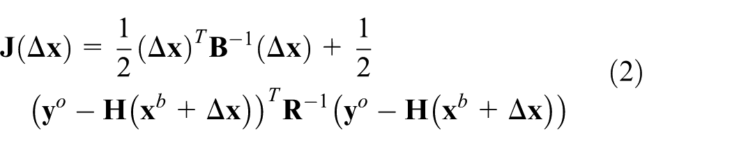
As for formula (2), incremental analysis $\mathrm{\Delta }\mathbf{x}$ is solved to find the minimum value of the cost function. In other words, the sensing of atmospheric parameters vector can be obtained.

For the multi-dimensional optimization problems mentioned above, Levenberg–Marquardt (LM) iteration method and Quasi-Newton (QN) iteration method are mainly used to solve the optimal solution to the cost function. ²³ Both methods must solve the first and second derivatives of the cost function. The LM method first solves the first and second derivative of the cost function, then iteratively calculates the matrix equation until the convergence criteria are satisfied. ²² Specifically, the form of matrix equation is

$$\mathbf{J}″({\mathbf{x}}^{i+1}-{\mathbf{x}}^i)=-\mathbf{J}\prime$$

(3)

where ${\mathbf{x}}^i$ and ${\mathbf{x}}^{i+1}$ are, respectively, the estimated value of the atmospheric parameter vectors of $i\mathrm{th}$ and $(i+1)\mathrm{th}$ iteration, while $\mathbf{J}\prime$ and $\mathbf{J}″$ are, respectively, the first and second derivatives of the cost function. The function will be expressed as follows

$$\mathbf{J}\prime \left(\mathbf{x}\right)={\mathbf{B}}^{-1}({\mathbf{x}}^i-{\mathbf{x}}^b)-\mathbf{H}{\left({\mathbf{x}}^i\right)}^T{\mathbf{R}}^{-1}({\mathbf{y}}^o-\mathbf{H}\left({\mathbf{x}}^i\right))$$

(4)

$$\mathbf{J}″\left(\mathbf{x}\right)\approx {\mathbf{B}}^{-1}+\mathbf{H}{\left({\mathbf{x}}^i\right)}^T{\mathbf{R}}^{-1}\mathbf{H}\left({\mathbf{x}}^i\right)$$

(5)

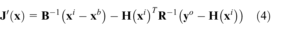
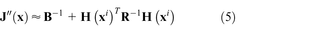
The minimum value of the cost function can be calculated by the LM method and the specific steps are the following:

1. Calculate the cost function $\mathbf{J}$ by formula (1) when the value of ${\mathbf{x}}^i$ is known;

2. Calculate $\mathbf{J}\prime$ and $\mathbf{J}″$ by using formulas (4) and (5) and then replace $\mathbf{J}″$ in formula (3) with $\mathbf{J}″·(1+\lambda )$ , where $\lambda$ is the proportionality coefficient and its initial value is usually set as 0.0001;

3. Solve formula (3) to obtain $d\mathbf{x}={\mathbf{x}}^{i+1}-{\mathbf{x}}^i$ and the atmospheric parameters vector ${\mathbf{x}}^{i+1}$ of the next iteration, to solve for a vector of atmospheric parameters;

4. Calculate $\mathbf{J}$ , the cost function corresponding to ${\mathbf{x}}^{i+1}$ . The iteration stops when $\mathbf{J}$ satisfies the stop condition. Otherwise, reduce λ when $\mathbf{J}$ reduces from the previous iteration, or increase λ when $\mathbf{J}$ increases from the previous iteration, so as to obtain $i=i+1$ . Repeat step 2, 3, and 4.

As shown by the above process, when the observation operator $\mathbf{H}(\mathbf{x})$ is complex, it is impossible to directly calculate the first and second derivative of the cost function, that is, $\mathbf{J}\prime$ and $\mathbf{J}″$ . As a result, LM method or QN method might fail to work. The solution is first to design the tangent linear and adjoint operators of the observation operators, and then reuse LM method or QN method to solve atmospheric parameters vector. It is difficult to design the tangent linear and adjoint operators; the LM method or QN method is also hard to achieve when the observation operator $\mathbf{H}(\mathbf{x})$ is quite complex.

Aiming at the shortcomings of the existing methods, this article provides a method to solve the sensing of atmospheric parameters based on simultaneous perturbation stochastic approximation (SPSA). SPSA uses perturbation to obtain the gradient approximation of the cost function, and gradually approximate the optimal solution. This method avoids calculating the first and second derivatives of the cost function, without designing tangent linear and adjoint operators, and guiding the search process to the optimal solution of the cost function by gradient approximation. These are the outstanding advantages of this method, compared with existing methods. It is also because of these advantages that this method provides a new method for solving the GPS RO variational data assimilation.

The data storage model of background field and observation operator

The data storage model of background field and observation operator

The atmospheric parameters vector of the background field is computed by ${\mathbf{x}}^b=(T,P,q{)}^T$ , where $T$ is the atmospheric temperature (unit: k), $P$ is the atmospheric pressure (unit: hPa), and $q$ is the atmospheric specific humidity (unit: g/kg). In this article, the background field data in the experiments are from the ECMWF, and the storage model is a vertical layer model shown in Figure 2. ²⁷ The atmosphere is divided into N layers, among which the $K\mathrm{th}$ layer stores the atmospheric temperature $T$ and specific humidity $q$ , and the $(K+1/2)\mathrm{th}$ layer (half layer) stores the atmospheric pressure coefficients $a_{k+1/2}$ and $b_{k+1/2}$ . The half-layer atmospheric pressure can be calculated by the surface atmospheric pressure and atmospheric pressure coefficients, and with the help of the half-layer atmospheric pressure, the whole-layer atmospheric pressure can be obtained.

Figure 2.

Vertical layer structure.

The half-layer and the whole-layer atmospheric pressure are calculated by

$$p_{k+1/2}=a_{k+1/2}+b_{k+1/2}·p_{\mathrm{sfc}}$$

(6)

$$p_k=\left(\frac{p_{k+1/2}+p_{k-1/2}}{2}\right)\left(0\le k\le N\right)$$

(7)

Another parameter to be calculated for each layer is its geopotential height. The geopotential height of both the half-layer and the whole layer is, respectively, calculated by

$$Z_{k+1/2}=Z_{\mathrm{sfc}}+\sum _{j=1}^k\frac{R_{\mathrm{dry}}{\left(T_v\right)}_j}{g_{\mathrm{wmo}}}\ln \left(\frac{p_{k-1/2}}{p_{k+1/2}}\right)$$

(8)

$$Z_k=Z_{k-1/2}+{\alpha }_k\frac{R_{\mathrm{dry}}{\left(T_v\right)}_j}{g_{\mathrm{wmo}}}(1\le k\le N)$$

(9)

where $Z_{\mathrm{sfc}}$ is the geopotential height of the surface atmospheric pressure, $R_{\mathrm{dry}}$ is the dry air constant, $T_v$ is the virtual temperature of each layer, and $g_{\mathrm{wmo}}$ is a reference gravity

$$T_v=T(1+\left(\frac{R_{\mathrm{vap}}}{R_{\mathrm{dry}}-1}\right)\times q)$$

(10)

$${\alpha }_k=1-\left(\frac{p_{k+1/2}}{\mathrm{\Delta }{p}_k}\right)\times \ln \left(\frac{p_{k-1/2}}{\mathrm{\Delta }{p}_{k+1/2}}\right)$$

(11)

$$\mathrm{\Delta }{p}_k=p_{k-1/2}-p_{k+1/2}$$

(12)

where $R_{\mathrm{vap}}$ is the water vapor constant.

Observation operator

Observation operator is utilized to map the atmospheric parameters vector of the model field to the observation field, and compare the atmospheric parameters with the observation data at a unified coordinate. Observation operator includes mapping function, interpolation function, and so on. The accuracy of the observation operator directly affects the accuracy of the results. According to different types of observation data, observation operator mainly can be divided into atmospheric refractivity operator and bending angle operator.

Atmospheric refractivity operator

The bending degree of GPS RO signal is determined by the refractivity index ( $n$ ) on the signal path. In practice, we usually use the atmospheric refractivity (N) that can be computed by the following formula

$$N=(n-1)\times {10}^6$$

(13)

Suppose the atmosphere has local spherical symmetry, the refractivity operator is expressed by $\mathbf{H}(\mathbf{x})=\mathbf{I}{\mathbf{H}}_N(\mathbf{x})$ , where ${\mathbf{H}}_N$ is the atmospheric refractivity which is calculated by the atmospheric temperature, pressure, and specific humidity of the background field, and $\mathbf{I}$ is the interpolation operator, which interpolates the atmospheric refractivity of the model field to the observation field.

Suppose the effects of non-ideal gas are ignored, the atmospheric refractivity $N$ is calculated by

$$N=u_1\frac{P}{T}+u{\prime }_2\frac{e}{T}+u_3\frac{e}{T^2}$$

(14)

where $e$ is the water vapor pressure, calculated by the pressure and specific humidity of the atmosphere, and $u_1$ , $u{\prime }_2$ , and $u_3$ are all empirical constants to determine by experiments.

Suppose $N$ changes in exponential form along with $x=\mathrm{nr}$ , where $r$ is the radius of curvature corresponding to the refractive index $(n)$ , the refractivity interpolation between $i\mathrm{th}$ and $(i+1)\mathrm{th}$ layers of the model field will be

$$N\left(x\right)=N_i\exp (-k_i(x-x_i))(x_i\le x\le x_{i+1})$$

(15)

where

$$k_i=\frac{\ln \left(\frac{N_i}{N_{i+1}}\right)}{x_{i+1}-x_i}$$

(16)

Algorithm 1: Atmospheric refractivity observation operator.

Calculate $T_v$ , $P$ , $e$ , $Z$ . // Calculate the atmospheric refractivity of the 137th layer $N_b=u_1\frac{p}{T}+u{\prime }_2\frac{p}{T}+u_3\frac{e}{T^2}$ Calculate $x_{\mathrm{bg}}=n_{\mathrm{bg}}·r_{\mathrm{bg}}$ , $x_0=n_0·r_0$ // Calculate the interpolation as follows. For $i=1:m$ // where $m$ is the dimension of the atmospheric refractivity.  For $j=1:137$  If $x_{\mathrm{bg}}(j)$  <  $x_o(i)$  <  $x_{\mathrm{bg}}(j+1)$    //Using interpolation formula to calculate $N_{b0}$   End  End End

$N_b$ is the atmospheric refractivity of the model field; $N_{b0}$ is the atmospheric refractivity mapping the model field to the observation field; $n_{\mathrm{bg}}$ and $n_0$ are, respectively, the atmospheric refractivity of the model field and observation field; and $r_{\mathrm{bg}}$ and $r_0$ are curvature radius corresponding to $n_{\mathrm{bg}}$ and $n_0$ , respectively.

One-dimensional bending angle operator

The study shows that the atmospheric parameters calculated by bending angle assimilation are more accurate and closer to the true value, but the bending angle operator is more complex than the atmospheric refractivity operator.

The bending angle is the total bending of the path of GPS signals when the signals pass through the neutral atmosphere. Suppose the atmosphere distribution is local spherical symmetric and the horizontal gradient variation of the atmosphere on the path of GPS signals are ignored, a one-dimensional (1D) bending angle operator can be modeled as

$$\alpha =H_a\mathbf{F}{\mathbf{H}}_N\left(\mathbf{x}\right)$$

(17)

where ${\mathbf{H}}_N$ is the atmospheric refractivity calculated by the temperature, humidity, and pressure of the atmosphere; $\mathbf{F}$ denotes that the atmospheric refractivity of the model field is interpolated to the observation field; and $H_a$ is the bending angle calculated according to the atmospheric refractivity. ⁶

The bending angle $\alpha (a)$ is a function of the impact parameter $a$ , and can be calculated by the Abel transform that can be precisely expressed as

$$\alpha \left(a\right)=-2a\underset{a}{\overset{\infty }{\int }}\frac{\frac{\mathrm{d}\left(\ln n\right)}{\mathrm{d}x}}{\sqrt{x^2-a^2}}\mathrm{d}x,$$

(18)

where $x=\mathrm{nr}$ . Suppose $N$ changes in exponential form along with $x=\mathrm{nr}$ , it can be deduced that $N(x)=N_i\exp (-k_i(x-x_i))$ . The bending angle between $i\mathrm{th}$ and $(i+1)\mathrm{th}$ layers is

$$\begin{array}{l}\mathrm{\Delta }\alpha ={10}^{-6}\sqrt{2\pi a{k}_i}{N}_i\exp \left(k_i\left(x_i-a\right)\right)\\ \times \left\{\mathrm{erf}\left(\sqrt{k_i\left(x_{i+1}-a\right)}\right)-\mathrm{erf}\left(\sqrt{k_i\left(x_i-a\right)}\right)\right\}\end{array}$$

(19)

the error function is given by

$$\mathrm{erf}\left(x\right)=\left(\frac{2}{\sqrt{\pi }}\right)\underset{0}{\overset{x}{\int }}{e}^{-t^2}\mathrm{dt}$$

(20)

The bending angle of the top layer is given by

$$\begin{array}{l}\mathrm{\Delta }\alpha \left(\mathrm{top}\right)={10}^{-6}\sqrt{2\pi a{k}_i}{N}_i\exp \left(k_i\left(x_{\mathrm{i}}-a\right)\right)\\ \times \left\{1-\mathrm{erf}\left(\sqrt{k_i\left(x_i-a\right)}\right)\right\}\end{array}$$

(21)

The bending angle $\alpha (a)$ with impact parameter $a$ is calculated as follows: first, the bending angle of each layer is calculated, and then $\alpha (a)$ can be obtained by adding the value of the bending angle from the top layer to the $(a+1)\mathrm{th}$ layer.

The error covariance matrices

In the cost function from equation (1), $\mathbf{B}$ is the error covariance matrix of the background field and $R$ is the error covariance matrix of observation field. If the assimilated GPS RO data are atmospheric refractivity, $R$ will be the error covariance matrix of the observed atmospheric refractivity. ²⁸ $\mathbf{B}$ is calculated by

$${\mathbf{B}}_{\mathrm{kl}}={\sigma }_k{\sigma }_l{\mathbf{C}}_{\mathrm{kl}}$$

(22)

where ${\sigma }_k$ and ${\sigma }_l$ are the standard deviations of the $k\mathrm{th}$ and the $l\mathrm{th}$ elements in the atmospheric parameter vectors of the background field, $\mathbf{C}$ is a constant matrix, and ${\mathbf{C}}_{\mathrm{kl}}$ represents the matrix element in the $k\mathrm{th}$ row and the $l\mathrm{th}$ column of $\mathbf{C}$ .

The error covariance matrix $\mathbf{R}$ of the observed atmospheric refractivity is given by

$${\mathbf{R}}_{\mathrm{ij}}={\sigma }_i{\sigma }_j\exp \left(\frac{-|{\mathrm{Z}}_i-{\mathrm{Z}}_j|}{h}\right)$$

(23)

where ${\sigma }_i$ and ${\sigma }_j$ are the standard deviations of the $i\mathrm{th}$ and the $(i+1)\mathrm{th}$ elements in the vector of the observation field; $Z_i$ and $Z_j$ are the geopotential heights of two observation values; and $h$ is an attenuation characteristic of correlation dimension. In most cases, the value of $h$ is 3 km. The error covariance matrix $\mathbf{R}$ of the bending angle is a diagonal matrix.

Quality Control

Before assimilating the GPS RO data into the NWP models, the GPS RO data quality must be tested to ensure that it reaches assimilation requirements and standards. There are plenty of methods for assessing the quality of GPS RO data. Generally speaking, the cost function ( $\mathbf{J}$ ) of GPS RO variational data assimilation system is subject to ${\chi }_m^2$ distribution. If $2\mathbf{J}/m>2$ (where $m$ is the dimension of the observation vector), the GPS RO data do not reach the assimilation standard. The quality of RO data published by a different institution using different satellite observation data is different. For example, the data, obtained by MetOp A and B, of atmospheric refractivity and bending angle whose geometric height is under 8 km and above 40 km might have big error and poor quality.

Improved SPSA algorithm for solving atmospheric parameter vector

SPSA, designed according to Kiefer-Wolfowitz ²⁹ (K-W), stochastic approximation algorithm has been proved to be an effective method of stochastic optimization. The algorithm uses the “gradient approximation” of a function to replace derivative, and guides the search process to approach the optimal solution. Meanwhile, this algorithm also has a positive effect on the treatment with measurement noise. Therefore, this algorithm is suitable for complex multidimensional optimization problems with observation noise and has been successfully applied to numerous fields.^29–33 In this article, SPSA is used to solve the minimal value of the cost function of GPS RO variational data assimilation. SPSA uses the gradient approximation of the cost function to replace the exact derivative. For this reason, there is no need to design the tangent linear and adjoint operators.

Basic principle of SPSA

The most significant feature of SPSA algorithm lies in being easy to accomplish and the efficient gradient approximation. ³¹ The basic principle is written as follows: suppose that $f(x)$ is a first-order continuous differentiable function for $x$ , $x^{*}$ that can make $f(x)$ obtain its minimum value can be solved. The formula procedure can be calculated by $g(x)=\mathrm{df}(x)/\mathrm{dx}$ , and $g(x^{*})=0$ . If the function of $f(x)$ is not a differentiable one, use the following recursion formula

$$x_k=x_{k-1}-a_k{g}_k\left(x_{k-1}\right)$$

(24)

where $x_k$ is the variable value of $k\mathrm{th}$ , $a_k$ is the choice of algorithm gain sequences, and $g_k(x_{k-1})$ is the gradient approximation of the function of $f(x)$ when $x=x_{k-1}$ .

The calculation process of SPSA algorithm mainly includes initialization, gradient estimation, updating variable values, and determining whether the requirements for stopping the algorithm are met or not.

Initialization

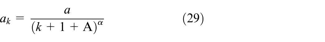
Set the initial iteration step length $a$ , initial perturbation factor $c$ , $\mathrm{A}$ , $\alpha$ , $\gamma$ , and non-negative coefficients in the SPSA gain sequences; typical values for $\alpha$ and $\gamma$ are 0.602 and 0.101; and $k_{max}$ is the maximum iterations in SPSA. Set the initial value (the value usually is ${\mathbf{x}}_o={\mathbf{x}}^b$ ) of the atmospheric parameter vector $\mathbf{x}$ , and the atmospheric parameters vector of the background field $\mathrm{\Delta }\mathbf{x}=(0,0,0{)}^T$ .

Gradient estimation

The key step of SPSA is to replace the exact solution to gradient (derivative) with the gradient estimation of the function. Each of gradient estimation only requires two measurement values. In this article, the gradient estimation of the cost function approximation to the unknown gradient $\mathbf{J}\prime$ is

$$\mathbf{J}\prime =({\mathbf{J}}^{+}-{\mathbf{J}}^{-})\times \frac{{|{\mathrm{\Delta }}_{\mathbf{k}1}^{-1},···,{\mathrm{\Delta }}_{\mathbf{kp}}^{-1}|}^{\mathbf{T}}}{(2•{\mathbf{c}}_{\mathbf{k}})}$$

(25)

where

$$\{\begin{array}{c}{\mathbf{J}}^{+}=\mathbf{J}(\mathbf{x}+{\mathbf{c}}_{\mathbf{k}}•{\mathrm{\Delta }}_{\mathbf{k}})\hfill \\ \multicolumn{1}{c}{{\mathbf{J}}^{-}=\mathbf{J}(\mathbf{x}-{\mathbf{c}}_{\mathbf{k}}•{\mathrm{\Delta }}_{\mathbf{k}})}\\ \multicolumn{1}{c}{{\mathbf{c}}_{\mathbf{k}}=\frac{\mathbf{c}}{{(\mathbf{k}+1)}^{\gamma }}}\end{array}$$

(26)

where ${\mathbf{J}}^{+}$ and ${\mathbf{J}}^{-}$ are two measurements of the cost function $\mathbf{J}$ based on the simultaneous perturbation around the current $\mathbf{x}$ , ${\mathrm{\Delta }}_k$ is the perturbation vector, and ${\mathrm{\Delta }}_k$ is ordinarily generated by Monte Carlo rule, for ${\mathrm{\Delta }}_k={|{\mathrm{\Delta }}_{k1},···,{\mathrm{\Delta }}_{\mathrm{kp}}|}^T$ , $p$ is the dimension of ${\mathrm{\Delta }}_k$ and the $p$ components of ${\mathrm{\Delta }}_k$ should satisfy for $\forall k$ ; $\left\{{\mathrm{\Delta }}_{\mathrm{ki}}\right\}$ is independently, identically distributed, and features in zero symmetry. We take the perturbations ${\mathrm{\Delta }}_k$ to be Bernoulli $\pm 1$ distributed and generated by a probability of 1/2. In order to improve the robustness of the algorithm on the condition of noise, the average gradient method is used to estimate the gradient

$$\mathbf{J}\prime ={\mathbf{q}}^{-1}\sum \mathbf{J}\prime$$

(27)

where $q$ is the number of gradient estimation.

Update atmospheric parameters vector

After calculating the approximate gradient of the function, we use the following formula to update the atmospheric parameters vector ${\mathbf{x}}_{k+1}$ ,

$${\mathbf{x}}_{k+1}={\mathbf{x}}_k+a_k\times \mathbf{J}\prime$$

(28)

where $\mathbf{J}\prime$ is the gradient approximation when $\mathbf{x}={\mathbf{x}}_k$ , and $a_k$ is the $k\mathrm{th}$ iterative step factor

$$a_k=\frac{a}{{(k+1+\mathrm{A})}^{\alpha }}$$

(29)

Iterative stopping judgment

If the number of current iteration is $k>k_{max}$ , or the current value of the cost function $\mathbf{J}({\mathbf{x}}_{i+1})$ has almost no evolution, the iteration will terminate. Otherwise, set $k=k+1$ and repeat 2, 3, and 4.

Algorithm 2: The SPSA algorithm.

For k = 0: $k_{max}$   $a_k=a/(k+1+\mathrm{A}){}^{\wedge }\mathrm{\alpha }$ , $c_k=c/(k+1{)}^{\wedge }\mathrm{\gamma }$  // $\mathrm{\Delta }$ generated by Monte Carlo rule as follows   $\mathrm{\Delta }$ = 2* round (rand (p, 1))-1   ${\mathbf{x}}^{+}={\mathbf{x}}_k+c_k*{\mathrm{\Delta }}_k$ , ${\mathbf{x}}^{-}={\mathbf{x}}_k-c_k*{\mathrm{\Delta }}_k$   ${\mathbf{J}}^{\prime }=(\mathbf{J}({\mathbf{x}}^{+})-\mathbf{J}(x^{-}))/(2\ast {\mathbf{c}}_{\mathbf{k}}\ast {\mathrm{\Delta }}_{\mathbf{k}}){\mathbf{x}}_{k+1}={\mathbf{x}}_k-a_k\ast {\mathbf{J}}^{\prime }$  If (( $|\mathbf{J}({\mathbf{x}}_{k+1})-\mathbf{J}({\mathbf{x}}_k)|<{\mathbf{J}}_{min}$ )|| $k>k_{max}$ )   Break  End End Output ${\mathbf{x}}_{k+1}$ , $\mathbf{J}({\mathbf{x}}_{k+1})$ , $k$ .

$a.*\mathbf{B}$ represents that the constant $a$ is multiplied by each element of the vector $\mathbf{B}$ while $a./\mathbf{B}$ represents that the constant $a$ is divided by each element of the vector $\mathbf{B}$ .

Improved SPSA algorithm

There are two types of situation where basic SPSA algorithm is used to solve atmospheric parameters vector:

1. The atmospheric parameters vector $\mathbf{x}=(T,P,q{)}^T$ includes atmospheric temperature, pressure, and specific humidity. Suppose ${\mathbf{x}}^l$ is the optimal solution to the atmospheric parameters vector, the final analysis increments will be $\mathrm{\Delta }{\mathbf{x}}^l={\mathbf{x}}^l-{\mathbf{x}}^b$ . In $\mathrm{\Delta }{\mathbf{x}}^l$ , the increments with different atmospheric parameters vary greatly in numerical value. When the basic SPSA algorithm uses uniform step-size factor to search each dimension of the vector to be solved, poor search efficiency can be found on some dimensions. For example, in certain bending angle assimilation, the analysis increment of the 40th layer is $\mathrm{\Delta }{\mathbf{x}}_{40}^l=(0.812,0.032,0.001)$ . This clearly shows that the three dimensions of the increment are quite different in terms of their value. If the SPSA algorithm uses a uniform step-size factor in the three-dimensional space, the convergence process of the algorithm will be longer.

2. The atmospheric parameters vector $\mathbf{x}=(T,P,q{)}^{\mathrm{T}}$ includes atmospheric temperature, pressure, and specific humidity. Take the atmospheric temperature, for example, suppose that the optimal solution is ${\mathbf{T}}^l=(T_1^l,\cdots ,T_p^l)$ , where $T_1^l,\cdots ,T_p^l$ are the optimal solutions to atmospheric temperature from the first layer to the $P\mathrm{th}$ layer. The atmospheric temperature vector of background field is ${\mathbf{T}}^b=(T_1^b,\cdots ,T_p^b)$ , where $T_1^b,\cdots ,T_p^b$ represent the atmospheric temperature from the first layer to the $P\mathrm{th}$ layer of the background field. The atmospheric temperature analysis increment is $\mathrm{\Delta }\mathbf{T}={\mathbf{T}}^l-{\mathbf{T}}^b=(T_1^l-T_1^b,\cdots ,T_p^l-T_p^b)$ . Elements of $\mathrm{\Delta }\mathbf{T}$ vary greatly with respect to numerical value. If this difference is ignored, the SPSA algorithm will also have a slow convergence speed in determining the initial step length.

In view of the above two cases, we make two improvements for the initial iterative step length $a$ of the basic SPSA algorithm. The two improvements are as follows:

1. Replace the initial iteration step length $a$ with an initial iteration vector $\mathbf{a}$ which has the same dimension as $\mathrm{\Delta }{\mathbf{x}}^l$ . The value of each element of $\mathbf{a}$ is determined according to the actual situation of the corresponding parameter. In the atmospheric refractivity assimilation, the corresponding elements of $\mathbf{a}$ , an initial iteration vector, and the atmospheric temperatures are set as follows: the atmospheric temperature vector of background field is $T^b=(T_1^b,\cdots ,T_p^b)$ , and the precision of each dimension of $T^b$ is determined. Suppose the precision of the atmospheric temperature of the $i\mathrm{th}$ layer is the $T_i^a$ , the corresponding atmospheric refractivity observations value will be $N_i^o$ . The temperature $T_i^c$ is determined by the interval $[T_i^b-T_i^a,T_i^b+T_i^a]$ centered at $T_i^b$ , which makes $|{N_i}^o-N_i^c|$ minimum; the formula is described by

   $$N_{\mathrm{i}}^c=u_1\frac{P_{\mathrm{i}}^b}{T_{\mathrm{i}}^c}+u{\prime }_2\frac{e_{\mathrm{i}}^b}{T_{\mathrm{i}}^c}+u_3\frac{e_{\mathrm{i}}^b}{{\left(T_{\mathrm{i}}^c\right)}^2}$$

   (30)

   where ${P_i}^b$ and ${e_i}^b$ are the corresponding atmospheric pressure and water vapor partial pressure of the background field. In the initial iteration vector $\mathbf{a}$ , the corresponding element of the atmospheric temperature $T_i^b$ is given by

   $${T_i}^b=\lambda ·|{T_i}^b-{T_i}^c|\lambda \in [0,1]$$

   (31)

2. In the GPS RO variational data assimilation, the calculus of the variations method is equivalent with the least-squares method. ³⁴ Suppose that the atmospheric temperature $T_r$ is the true value, $T^b$ is the atmospheric temperature of background field, and its variance is the ${\sigma }_b^2$ , and $T^o$ is the atmospheric temperature of observation field, and its variance is the ${\sigma }_o^2$ .

$$\{\begin{array}{c}{T}^b=T_r+{\epsilon }_1\hfill \\ \multicolumn{1}{c}{T^o=T_r+{\epsilon }_2}\end{array}$$

(32)

where ${\epsilon }_1$ and ${\epsilon }_2$ are noises. The least-squares method for solving the optimal temperature $T$ is written by

$$T_{\mathrm{ls}}=\left[\frac{{\sigma }_o^2}{({\sigma }_b^2+{\sigma }_o^2)}\right]*T^b+\left[\frac{{\sigma }_b^2}{({\sigma }_b^2+{\sigma }_o^2)}\right]*T^o$$

(33)

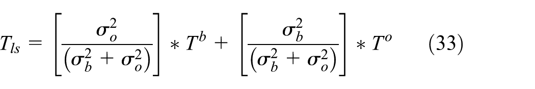
The process of solving the optimum solution to temperature by variational calculus is to find the temperature $T_{\mathrm{vs}}$ which makes the cost function $J(T)=(T-T^b{)}^2/{\mathrm{\sigma }}_b^2+(T-T^o{)}^2/{\mathrm{\sigma }}_o^2$ minimum. When $J\prime (T)=\partial J/\partial T$ and $J\prime (T_{\mathrm{vs}})=0$ , $J\prime (T_{\mathrm{vs}})$ can be expanded as

$$J\prime \left(T_{\mathrm{vs}}\right)=\frac{2(T_{\mathrm{vs}}-T^b)}{{\sigma }_b^2}+\frac{2(T_{\mathrm{vs}}-T^o)}{{\sigma }_o^2}=0$$

(34)

$$T_{\mathrm{vs}}=\frac{{\sigma }_o^2*T^b}{({\sigma }_b^2+{\sigma }_o^2)}+\frac{{\sigma }_b^2*T^o}{({\sigma }_b^2+{\sigma }_o^2)}$$

(35)

It is obvious that $T_{\mathrm{ls}}=T_{\mathrm{vs}}$ , namely, the calculus of variations method and the least-squares method are equivalent. And it can be seen from the expressions of $T_{\mathrm{ls}}$ and $T_{\mathrm{vs}}$ that the optimal estimation is closer to the smaller standard deviation.

Suppose the initial step length of temperature ( $T$ ) is $\mathbf{a}(T)$ . According to the difference of the variance, $\mathbf{a}(T)$ is adjusted by the following formula

$$\mathbf{a}\left(T\right)=\{\begin{array}{c}3*\mathbf{a}\left(T\right)({{\sigma }_b}^2>3*{{\sigma }_o}^2)\hfill \\ \multicolumn{1}{c}{\mathbf{a}\left(T\right)*\frac{{\sigma }_o^2}{{\sigma }_b^2}({{\sigma }_o}^2\le {{\sigma }_b}^2\le 3*{{\sigma }_o}^2)}\\ \multicolumn{1}{c}{\mathbf{a}\left(T\right)*\frac{{\sigma }_b^2}{{\sigma }_o^2}({{\sigma }_b}^2<{{\sigma }_o}^2)}\end{array}$$

(36)

The improved SPSA algorithm replaces the initial iteration step length $a$ with an initial iteration vector $\mathbf{a}(T)$ , and does optimization settings according to formula (36). This is helpful to improve the convergence speed of the algorithm, so that the algorithm could quickly and accurately solve atmospheric parameters vector.

Algorithm 3: Set the initial step-size vector $\mathbf{a}(T)$ of temperature vector ( $T$ ).

For i = 1:137//the number of 137 is the layer of temperature  //vector $T$  Set the calculation interval $[T_i^b-T_i^a,T_i^b+T_i^a]$  Calculate the interval of atmospheric refractivity $[N_i^1,N_i^2]$  If ( $N_i^o>N_i^1$ ) $T_i^c=T_i^2$ ; // $T_i^1$ corresponding to $N_i^1$  Else if ( $N_i^o>N_i^2$ ) $T_i^c=T_i^2$ ; // $T_i^2$ corresponding to $N_i^1$  Else $T_i^c=T_i^o$ ; // $T_i^o$ corresponding to $N_i^c$  End If ( $T_i^c$ have multiple values)  The values of $T_i^c$ that make the formula $|T_i^b-T_i^c|$ reach the minimum value. End $\mathbf{a}(T_i^b)=\lambda ·|T_i^b-T_i^c|$ ; If ( $({{\sigma }_i}^{\mathrm{b}}{)}^2>3*({{\sigma }_i}^{\mathrm{c}}{)}^2$ ) $\mathbf{a}(T_i^b)=3*\mathbf{a}(T_i^b)$ ; Else if ( $({{\sigma }_i}^{\mathrm{c}}{)}^2<({{\sigma }_i}^{\mathrm{b}}{)}^2\le 3*({{\sigma }_i}^{\mathrm{c}}{)}^2$ )   $\mathbf{a}({T_i}^{\mathrm{b}})=\mathbf{a}({T_i}^{\mathrm{b}})*({{\sigma }_i}^{\mathrm{b}}{)}^2/({{\sigma }_i}^{\mathrm{o}}{)}^2$ ;  Else   $\mathbf{a}({T_i}^{\mathrm{b}})=\mathbf{a}({T_i}^{\mathrm{b}})*({{\sigma }_i}^o{)}^2/({{\sigma }_i}^{\mathrm{b}}{)}^2$ ;;  End End

${{\sigma }_i}^{\mathrm{b}}$ is the standard deviation of the background field of atmospheric temperature $T_i^b$ , ${{\sigma }_i}^{\mathrm{c}}$ is the standard deviation of the $T_i^c$ , and $\mathbf{a}(T_i^b)$ is the initial iteration step size corresponding to $T_i^b$ .

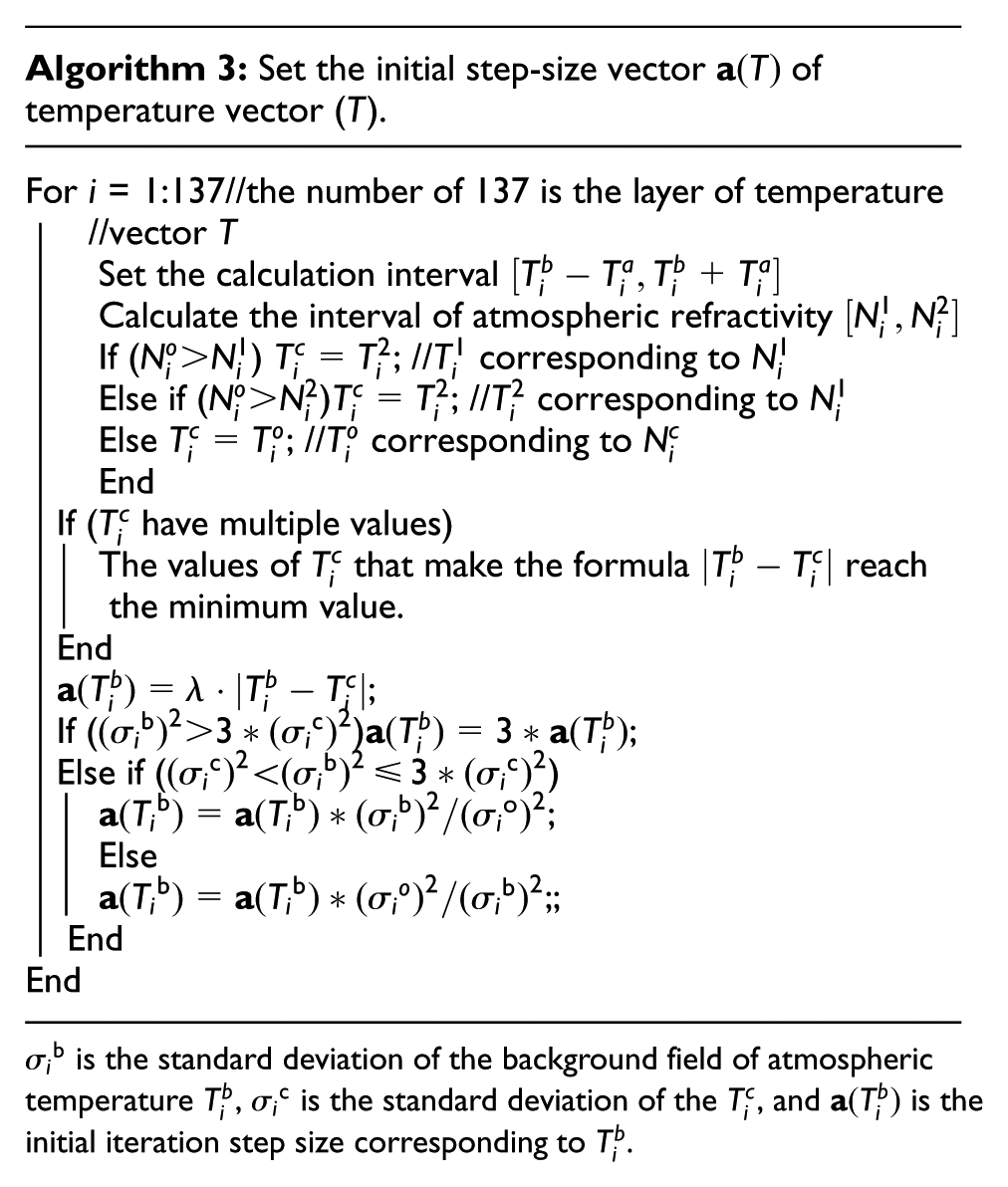
The process of using the improved SPSA algorithm to solve the atmospheric parameter vector is as follows: first, pre-process data, including the calculation of atmospheric pressure and geopotential height; second, test the data quality, if the data meet the assimilation standard, do assimilation. Otherwise, stop the solving process; use the improved SPSA algorithm to calculate the minimal value of the cost function in formula (2) so as to obtain the sensing of atmospheric parameters vector and output the results.

Experiment analysis

In order to verify the effectiveness of the improved SPSA algorithm for solving the atmospheric parameter vector, two sets of experiment are carried out in this article. One is the one-dimensional atmospheric refractivity assimilation experiment and the other is the one-dimensional bending angle assimilation experiment. Afterward, a comprehensive comparison with existing methods is conducted.

One-dimensional atmospheric refractivity assimilation experiments

In the one-dimensional atmospheric refractivity assimilation experiment, we adopt a set of background field data from ECMWF in March 2015, and use observation data of atmospheric refractivity of LEO MetOp satellites. The algorithm of this article is used to solve the atmospheric parameters vector (temperature, pressure, and specific humidity). The algorithm is run for 50 times to obtain statistical results. Besides, a comparison between the algorithm and the LM method is also carried out. ²² The parameters setting of the algorithm of this article is shown in Table 1.

Table 1.

The parameters setting of the SPSA.

Parameters	$A$	$\alpha$	$\gamma$	$k_{max}$	$\lambda$
Values	1	0.602	0.101	25	0.05

SPSA: simultaneous perturbation stochastic approximation.

In a high-noise setting, it is necessary to pick a small $\alpha$ and large $\mathrm{c}$ than in a slow-noise setting. Although the asymptotically optimal values of $\alpha$ and $\gamma$ are 1.0 and 1/6, it appears that choosing $\alpha <1.0$ usually yields better finite-sample performance through maintaining a larger step size, hence the values 0.0602 and 0.101 shown in Table 1. A guideline we have found useful is to choose $A$ such that it is much less than the maximum number of iterations allowed or expected; we frequently take it to be 10% (or less) of the maximum number of expected/allowed iterations, hence in the Table 1 set, $A=1$ . When the occultation data are assimilated, it can be up to 25 iterations. If the number of iterations is exceeded, the optimal solution of the atmospheric parameters is considered to be unsatisfactory. The value of $c$ should be as close to the measurement noise deviation as possible, and when there is no noise in the environment, the value of $c$ can be a small positive number.

It shows the evolutionary curves of the cost function of the atmospheric parameter vector solved by SPSA algorithm (Figure 3). The two curves represent the results of the basic SPSA algorithm and the improved SPSA algorithm (average of 50 runs). Vertical lines indicate the floating range of the cost function value in each iteration. It is obvious that improved SPSA algorithm converges faster, that the solution to the cost function value is ultimately smaller, and that the running stability is better.

Figure 3.

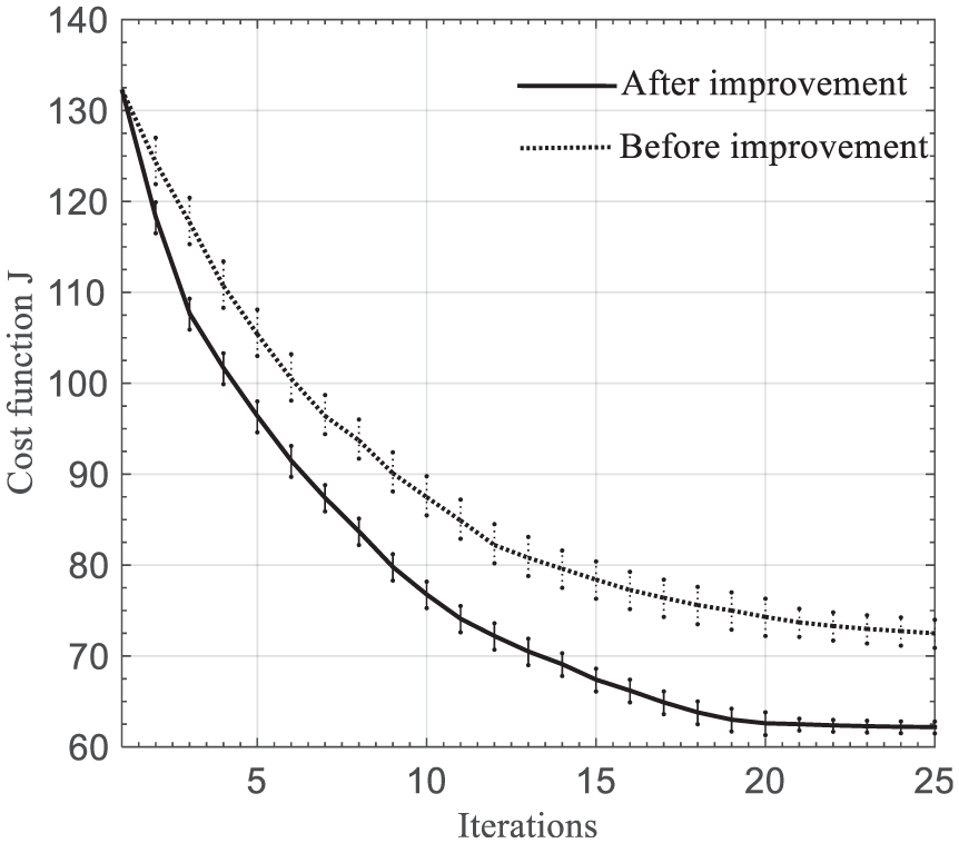
Evolutionary curve of cost function of SPSA algorithm for the sensing of atmospheric parameter vector.

The performance comparison, from the perspective of multi aspects, between the algorithm in this article and the LM method is shown in Table 2. It can be seen that the cost function value solved by the algorithm in this article, especially its average (62.2937), is less than the cost function average (62.8346) solved by the LM method. Hence, the atmospheric parameter figured out by the algorithm of this article is more statistically optimal.

Table 2.

The comparison between improved SPSA algorithm and LM method.

Method	Improved SPSA	LM
Maximum	62.9261	62.8346
Minimum	61.6614	62.8346
Average	62.2937	62.8346

SPSA: simultaneous perturbation stochastic approximation; LM: Levenberg–Marquardt.

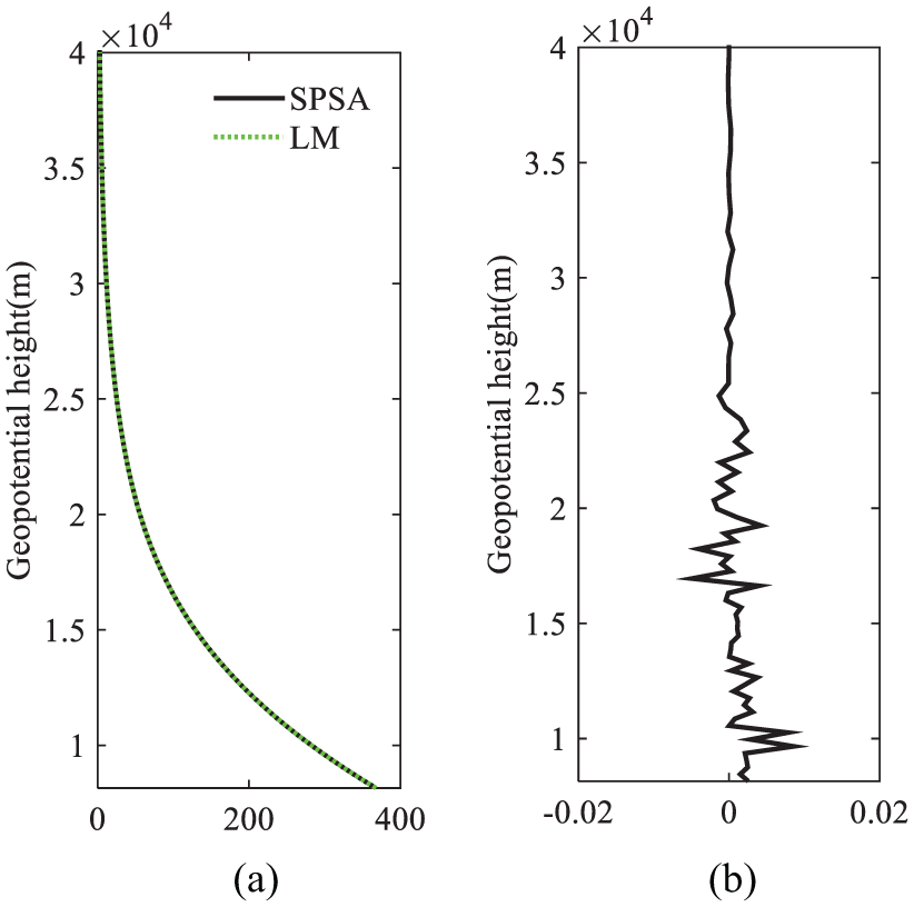
The results of the atmospheric temperature, pressure, and specific humidity solved by the algorithm of this article and LM method are presented in Figures 4–6. Figure 4(a) shows that the atmospheric temperature profiles of the two methods (the atmospheric temperature distribution profiles of different geopotential heights) almost coincide and have a good consistency. Figure 4(b) shows the differences between the values of atmospheric temperature of the two methods. The differences are less than 0.2 K, and most of them are within 0.05 K. These further demonstrate the consistency of the results of the two methods. The cost function value of the algorithm of this article is smaller so that the results are closer to the true value of the atmospheric temperature.

Figure 4.

On March 1, 2015, ECMWF published a set of atmospheric background data from 12:00 at 30°N, 117°E, from GPS/MET data for statistical analysis of atmospheric parameters of each layer. The average atmospheric temperature was calculated using the LM and SPSA algorithms. The problem that causes the peak of Figure 4(a) is the junction of the stratosphere and the troposphere. (a) atmospheric temperature (K); (b) the difference values of the two methods (K).

Figure 5.

On March 1, 2015, ECMWF published a set of atmospheric background data from 12:00 at 30°N, 117°E, from GPS/MET data for statistical analysis of atmospheric parameters of each layer. The average atmospheric pressure was calculated using the LM and SPSA algorithms. (a) atmospheric pressure (hPa); (b) the difference values of the two methods (hPa).

Figure 6.

On March 1, 2015, ECMWF published a set of atmospheric background data from 12:00 at 30°N, 117°E, from GPS/MET data for statistical analysis of atmospheric parameters of each layer. The average atmospheric humidity was calculated using the LM and SPSA algorithms. (a) atmospheric humidity (g/Kg); (b) the difference values of the two methods (g/Kg).

Figure 5 shows the consistency of the two methods for solving atmospheric pressure, and the differences of the atmospheric pressure are less than 0.0065 hPa. Figure 6 shows the consistency of the two methods for solving atmospheric specific humidity, and the differences of the atmospheric specific humidity are less than 0.0002 g/Kg.

In summary, in the one-dimensional atmospheric refractivity assimilation experiment, the improved SPSA algorithm for solving atmospheric parameters vector can not only obtain faster convergence and higher quality than basic SPSA algorithm but also can achieve a solution whose value is closer, compared with that of LM method, to the true value of atmospheric parameters. Furthermore, as the SPSA algorithm avoids complex cost function derivation process, the algorithm is easier to accomplish.

One-dimensional bending angle experiment types of graphics

The algorithm of this article is used to solve the atmospheric parameters vector (temperature, pressure, and specific humidity). The algorithm is run for 50 times to obtain statistical results, which is compared with that of the LM method. We used different $\lambda$ values in different experiments to verify whether it affected the performance of the experiment, so we fixed $\lambda =0.02$ , and other parameters are shown in Table 1.

Figure 7 shows the evolutionary curves of the cost function of the atmospheric parameter vector solved by SPSA algorithm. The two curves represent the results of the basic SPSA algorithm and the improved SPSA algorithm (average of 50 runs). It can be told that improved SPSA algorithm converges faster, that the ultimate solution to the cost function value is smaller, and that the running stability is better.

Figure 7.

Evolutionary curve of cost function of SPSA algorithm for the sensing of the atmospheric parameter vector.

The performance comparison, in terms of multi-aspects, between the algorithm in this article and the LM method is shown in Table 3. It can be seen that the cost function value solved by the algorithm in this article, especially its average (56.675), is less than the cost function average (57.756) solved by the LM method. The algorithm of this article figures out a more statistically optimal atmospheric parameter.

Table 3.

Comparison of improved SPSA algorithm and LM method.

Method	Improved SPSA	LM
Maximum	58.124	57.756
Minimum	55.226	57.756
Average	56.675	57.756

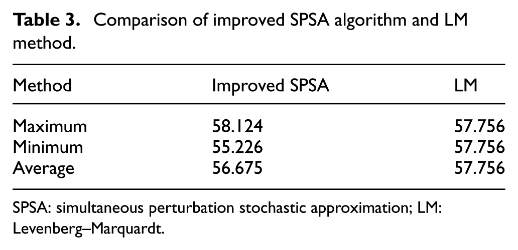
SPSA: simultaneous perturbation stochastic approximation; LM: Levenberg–Marquardt.

The results of the atmospheric temperature, pressure, and specific humidity solved by the algorithm of this article and LM method are shown in Figure 8–10. Figure 8(a) shows that the atmospheric temperature profiles of the two methods have a good consistency. Figure 8(b) shows the differences between the values of atmospheric temperature of the two methods. The differences are less than 0.25 K, and most of them are less than 0.1 K. These further demonstrate the consistency of the results of the two methods. The cost function value of the algorithm of this article is smaller, which proves the results of the algorithm are closer to the true value of the atmospheric temperature.

Figure 8.

On March 1, 2015, ECMWF published a set of atmospheric background data from 12:00 at 30°N, 117°E, from GPS/MET data for statistical analysis of atmospheric parameters of each layer. The average atmospheric temperature was calculated using the LM and SPSA algorithms. The problem that causes the peak of Figure 8(a) is the junction of the stratosphere and the troposphere. (a) atmospheric temperature (K); (b) the difference values of the two methods (K).

Figure 9.

On March 1, 2015, ECMWF published a set of atmospheric background data from 12:00 at 30°N, 117°E, from GPS/MET data for statistical analysis of atmospheric parameters of each layer. The average atmospheric pressure was calculated using the LM and SPSA algorithms. (a) atmospheric pressure (hPa); (b) the difference values of the two methods (hPa).

Figure 10.

On March 1, 2015, ECMWF published a set of atmospheric background data from 12:00 at 30°N, 117°E, from GPS/MET data for statistical analysis of atmospheric parameters of each layer. The average atmospheric humidity was calculated using the LM and SPSA algorithms. (a) atmospheric humidity (g/Kg); (b) the difference values of the two methods (g/Kg).

Figure 9 shows the consistency of the two methods for solving the atmospheric pressure, and the differences of the atmospheric pressure are less than 0.005 hPa. Figure 10 shows the consistency of the two methods for solving the atmospheric specific humidity, and the differences of the atmospheric specific humidity are less than 0.0002 g/Kg.

In summary, in the one-dimensional bending angle assimilation experiment, the improved SPSA algorithm for solving atmospheric parameters vector can not only make faster convergence and higher quality than basic SPSA algorithm, but also obtain the results whose value is closer, than that of LM method, to the true value of the atmospheric parameters.

One-dimensional bending angle experiment types of graphics: comparing computational costs for one-dimensional bend angles

Based on the one-dimensional bending angle experiment, we compared the computational cost of improved SPSA algorithm and LM methods and recorded the running time of the two algorithms, respectively. The statistical CPU(s) runtimes are shown in Table 4.

Table 4.

Comparison of improved SPSA algorithm and LM method.

Method	Count 10 CPU(s) runtimes					Average
Improved SPSA	0.034	0.035	0.035	0.032	0.032	0.336
LM	0.083	0.082	0.082	0.080	0.084	0.0822

SPSA: simultaneous perturbation stochastic approximation; LM: Levenberg–Marquardt.

In addition, in using the LM method to solve atmospheric parameters vector, the tangent and adjoint operators of the one-dimensional bending angle must be designed. Consequently, the process is quite complex. In the three-dimensional and four-dimensional variational data assimilation system, the design of the tangent and adjoint operators are more difficult and complex, and the process to calculate the first and second derivatives of the cost function is pretty complicated, too. Hence, the LM method is more difficult to apply to bending angle assimilation.

By contrast, the algorithm of this article avoids designing the tangent linear and adjoint operators, replaces the first- and second-order derivatives with the gradient approximation of the cost function, and guides the search process with the help of gradient approximation to gradually approach the optimal solution. Moreover, the algorithm in this article is easier to implement and is of higher accuracy.

Conclusion

This article studies the problems about GPS RO data assimilation for solving atmospheric parameters, and provides an improved SPSA method for solving atmospheric parameters. In this method, the first step is to determine the experimental parameters in accordance with the data characteristics of the background field and observation field and their error covariance; then “perturbation” is used to obtain the gradient approximation of the cost function; finally, this method guides the iterative search process to gradually approach the atmospheric parameters vector.

Both the one-dimensional atmospheric refractivity assimilation experiment and the one-dimensional bending angle assimilation experiment results prove that the improved SPSA algorithm, compared with LM method, has faster convergence speed and the advantages, such as higher quality and being easy to implement.

This article introduces the variational data assimilation techniques into the SPSA algorithm, which enriches the methodology system for solving the cost function method. Based the characteristics of variational data assimilation cost function, the basic SPSA algorithm is improved to increase its solving efficiency and quality. The future work is to expand the application of this method to the “nonlocal” assimilation of GPS RO data and verify the comprehensive effectiveness of this method.