Adaptive fitting algorithm of progressive interpolation for Loop subdivision surface

Abstract

Subdivision surface and data fitting have been applied in data compression and data fusion a lot recently. Moreover, subdivision schemes have been successfully combined into multi-resolution analysis and wavelet analysis. This makes subdivision surfaces attract more and more attentions in the field of geometry compression. Progressive interpolation subdivision surfaces generated by approximating schemes were presented recently. When the number of original vertices becomes huge, the convergence speed becomes slow and computation complexity becomes huge. In order to solve these problems, an adaptive progressive interpolation subdivision scheme is presented in this article. The vertices of control mesh are classified into two classes: active vertices and fixed ones. When precision is given, the two classes of vertices are changed dynamically according to the result of each iteration. Only the active vertices are adjusted, thus the class of active vertices keeps running down while the fixed ones keep rising, which saves computation greatly. Furthermore, weights are assigned to these vertices to accelerate convergence speed. Theoretical analysis and numerical examples are also given to illustrate the correctness and effectiveness of the method.

Introduction

Wireless multimedia sensor network (WMSN) ¹ is a network of wirelessly interconnected sensor nodes equipped with multimedia devices, such as cameras, microphones, and other sensors. Compared to traditional wireless sensor networks (WSNs), ² WMSNs can sense the multimedia information such as retrieve videos and audio streams, still images, and scalar sensor data. Recently, it has been widely applied in both civilian and military areas which require visual and audio information such as surveillance sensor networks, law-enforcement reports, traffic control systems, advanced health-care delivery, automated assistance to elderly telemedicine, and industrial process control. Sensor nodes of WMSNs have low computation capability, small memory, and limited energy performances. This makes WMSNs suffer from many constraints, including susceptibility to physical capture, tremendous transmission of multimedia data, and the use of insecure wireless communication channels. Moreover, when sensor nodes collect regional information and upload them to the base station, there are plenty of redundant data in the process of uploading. As the various applications of WMSNs increase, these problems become more complex. Furthermore, WMSNs have additional requirements such as in-node (sensor node) multimedia processing techniques (e.g. distributed multimedia source coding and data compression^3–5), application-specific quality of service (QoS) requirements, ⁶ and multimedia in-network processing techniques (e.g. storage management, data fusion, and data aggregation^7–11). Subdivision surface and data fitting have been applied in data processing techniques (data aggregation, data compression, and data fusion) a lot recently. The application of these technologies on sensors will alleviate the shortcomings of sensors and reduce the limitations of WSNs. Moreover, with the development of the second-generation wavelet analysis and multi-resolution transmission framework theory, subdivision schemes have been successfully combined into multi-resolution analysis and wavelet analysis. This makes subdivision surfaces attract more and more attentions in the field of geometry compression.

Subdivision surfaces refer to a class of modeling schemes which define objects by refining certain initial control meshes. ¹² Subdivision surfaces are easy to implement, they can model surfaces of arbitrary topological type, and the continuities of these surfaces can be controlled locally. A subdivision scheme is called an interpolating one if the limit surface interpolates the given control mesh, such as Butterfly and Kobbelt schemes.^13,14 Otherwise, it is called an approximating scheme, such as Catmull–Clark, Doo–Sabin, and Loop schemes.^15–17 Approximating subdivision surface usually has better quality than that of interpolating one, but approximating method is unable to interpolate the vertices of the initial control mesh. Traditional methods which make the approximating subdivision surface interpolate the initial mesh need to solve a global linear system.^18,19 It is computation intensive and hard to deal with dense meshes. Progressive–iterative approximation (PIA) method has been introduced to solve these kinds of problems. It was first presented by Qi et al. ²⁰ and De Boor ²¹ which was called the “profit and loss” method for cubic B-spline. Lin et al. ²² proved the convergence in 2004. Later, Lin et al. ²³ generalized the method which showed that the algorithm is convergent for normalized and totally positive basis, and formally named the method as PIA method. Recently, Lin and colleagues^24–27 applied the method in many areas. Recently, Cheng et al.,^12,28 Chen et al., ²⁹ and Deng and Ma ³⁰ introduced PIA method into subdivision schemes. Without solving linear system of equations, these methods calculate the approximating subdivision surfaces that interpolate the initial meshes by adjusting the vertices of control meshes iteratively. It can handle control meshes of any size and any topology while generating smooth subdivision surfaces that faithfully resemble shapes of initial meshes. But there are still a few troubles to overcome. When the number of original vertices becomes huge, the convergence speeds become slow and computation complexity becomes huge. In order to solve these problems, adaptive progressive interpolation subdivision scheme is proposed in this article. The vertices of control mesh are classified into two classes: active vertices and fixed ones. These two classes of vertices are changed dynamically according to the result of each iteration when precision is given. Only the active vertices are adjusted, thus the number of active vertices keeps running down while the number of fixed ones keeps rising, which saves computation greatly.

The main contributions of the article are listed as follows:

1. Adaptive data fitting algorithm is presented in this article; it can handle large-scale data points and save computation greatly.

2. Weighted adaptive algorithm is also presented here in order to control the convergence rate adaptively.

3. The algorithm possesses the common advantages of adaptive data fitting algorithm and weighted adaptive algorithm.

This article is organized as follows. Theory basis of the algorithm is presented in section “Local weighted progressive interpolation algorithm for Loop subdivision surfaces.” Fitting precision analysis is given in section “Fitting precision analysis.” In section “Adaptive data fitting algorithm and weighted adaptive algorithm,” adaptive data fitting algorithm and weighted adaptive algorithm for Loop subdivision surfaces are given. Plenty of experimental examples are illustrated in section “Numerical examples.” Conclusions are drawn in section “Conclusion.”

Local weighted progressive interpolation algorithm for Loop subdivision surfaces

Zhao et al. ³¹ have shown that progressive interpolation subdivision schemes can interpolate vertices globally or locally according to different application backgrounds. Local property of progressive interpolation brings more flexibility for shape control and makes adaptive fitting process possible. Local weighted progressive interpolation algorithm for Loop subdivision surfaces is proposed, which can be applied to the other approximating subdivision surfaces. The process of local weighted progressive interpolation is as follows.

Given a triangular mesh $M^0=\{V_1^0,V_2^0,\dots ,V_n^0\}$ . The initial control vertices are divided into two subsets: the fixed set $\{V_j\}$ , $j\in J=\{j_0,j_1,\dots ,j_J\}$ , in which the difference vector is less than the given threshold, and the active set $\left\{V_i\right\}$ , $i\in I=\{i_0,i_1,\dots ,i_I\}$ , in which the difference vector is greater than the given threshold. Operations are only applied on the active set and leave the fixed one invariant.

After k iteration, we can get the kth triangular mesh $M^k=\{V_1^k,V_2^k,\dots ,V_n^k\}$ and the corresponding vertices $V_j^k,j\in J=\{j_0,j_1,\dots ,j_J\}$ and $V_i^k,i\in I=\{i_0,i_1,\dots ,i_I\}$ . Then, $M^{k+1}$ is obtained by the following operation. For the active vertices $(V_i^k,i\in I=\{i_0,i_1,\dots ,i_I\})$

$$D_i^k=V_i^0-V_i^{k,\infty }$$

(1)

$$V_i^{k+1}=V_i^k+w{D}_i^k$$

(2)

where $w$ is the weight which is a positive real number between 0 and 2. After modifying each vertex in the active set, we get $M^{k+1}=\{V_1^{k+1},V_2^{k+1},\dots ,V_n^{k+1}\}$ .

By repeating the above process, a sequence of meshes $M^k(k=1,2,\dots )$ is obtained. Defining function

$$H(V_i,V_j)=\{\begin{array}{cc}1,\hfill & V_j\mathrm{is}\mathrm{an}\mathrm{active}\mathrm{vertex}\mathrm{which}\mathrm{adjacent}\mathrm{to}{V}_i\hfill \\ \multicolumn{1}{c}{0,}& \mathrm{others}\hfill \end{array}$$

Let ${\mathbf{D}}_I^k=[D_{i_0}^k,D_{i_1}^k,\dots ,D_{i_I}^k{]}^T$ be the set for active difference vectors and ${\mathbf{D}}_J^k=[D_{j_0}^k,D_{j_1}^k,\dots ,D_{j_J}^k{]}^T$ be the set for fixed ones. These two sets will converge when iteration steps tend to infinity.

Theorem 1

As k tends to infinity, ${\mathbf{D}}_I^k$ tends to zero, and ${\mathbf{D}}_J^k$ tends to ${\mathbf{D}}_J^0+w\mathbf{C}{\overline{\mathbf{B}}}^{-1}{\mathbf{D}}_I^0$ , where

$$\overline{\mathbf{B}}=\left(\begin{array}{cccc}{\beta }_{n_{i_0}}\hfill & \cdots \hfill & \frac{1-{\beta }_{n_{i_0}}}{n_{i_0}}H(V_{n_{i_0}},V_{n_{i_k}})\hfill & \cdots \hfill \\ \multicolumn{1}{c}{⋮}& \ddots \hfill & \hfill & \hfill \\ \multicolumn{1}{c}{\frac{1-{\beta }_{n_{i_k}}}{n_{i_k}}H(V_{n_{i_0}},V_{n_{i_k}})}& \cdots \hfill & {\beta }_{n_{i_k}}\hfill & \cdots \hfill \\ \multicolumn{1}{c}{⋮}& \hfill & \hfill & {\beta }_{n_{i_I}}\hfill \end{array}\right)$$

$$\mathbf{C}=\left(\begin{array}{cccc}-\frac{1-{\beta }_{n_{j_0}}}{n_{j_0}}{H}_{j_0,i_0}\hfill & -\frac{1-{\beta }_{n_{j_0}}}{n_{j_0}}{H}_{j_0,i_1}\hfill & \cdots \hfill & -\frac{1-{\beta }_{n_{j_0}}}{n_{j_0}}{H}_{j_0,i_I}\hfill \\ \multicolumn{1}{c}{-\frac{1-{\beta }_{n_{j_1}}}{n_{j_1}}{H}_{j_1,i_0}}& -\frac{1-{\beta }_{n_{j_1}}}{n_{j_1}}{H}_{j_1,i_1}\hfill & \cdots \hfill & -\frac{1-{\beta }_{n_{j_1}}}{n_{j_1}}{H}_{j_1,i_I}\hfill \\ \multicolumn{1}{c}{⋮}& ⋮\hfill & \hfill & ⋮\hfill \\ \multicolumn{1}{c}{-\frac{1-{\beta }_{n_{j_J}}}{n_{j_J}}{H}_{j_J,i_0}}& -\frac{1-{\beta }_{n_{j_J}}}{n_{j_J}}{H}_{j_J,i_1}\hfill & \cdots \hfill & -\frac{1-{\beta }_{n_{j_J}}}{n_{j_J}}{H}_{j_J,i_I}\hfill \end{array}\right)$$

$${\beta }_{n_{i_k}}=\frac{3}{11-8\times (\frac{3}{8}+{(\frac{3}{8}+\frac{1}{4}\cos \frac{2\pi }{n_{i_k}})}^2)},H_{j,i}=H(V_j,V_i)$$

Proof

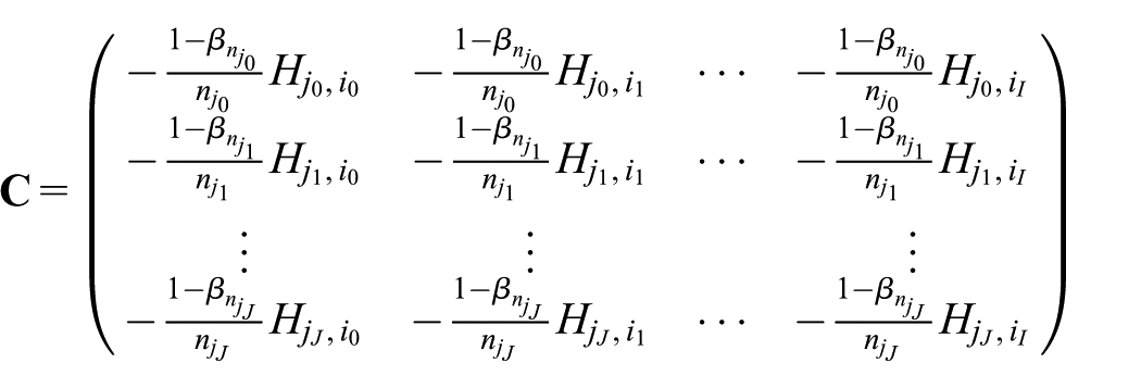
For the active vertices set, that is, $i\in I=\{i_0,i_1,\dots ,i_I\}$ , we have

$$D_i^{k+1}=V_i^0-V_{i,\infty }^{k+1}=V_i^0-({\beta }_n{V}_i^{k+1}+(1-{\beta }_n){Q_i}^{k+1})$$

By equations (1), (2), and ${Q_i}^{k+1}=Q_i^k+w\frac{1}{n}\sum _{l\in I_i}{D}_{Q_{i,l}^k}^k$ , we can get the relationship between $D_i^{k+1}$ and $D_i^k$ as

$$D_i^{k+1}=D_i^k-w({\beta }_n{D}_i^k+\frac{1-{\beta }_n}{n}\sum _{l\in I_i}{D}_{Q_{i,l}^k}^k)$$

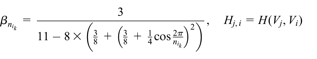
where n is the valence of vertices $V_i^k$ . ${Q_i}^k$ and $Q_{i,l}^k$ are the active vertices which are adjacent to the vertex $V_i^k$ . $I_i$ is the active index set which is also adjacent to $V_i^k$ . It has the following matrix form

$${\mathbf{D}}_I^{k+1}=(\mathbf{E}-w\overline{\mathbf{B}}){\mathbf{D}}_I^k={(\mathbf{E}-w\overline{\mathbf{B}})}^{k+1}{\mathbf{D}}_I^0$$

(3)

It has been proved that $0<\lambda (\overline{\mathbf{B}})<1$ . ²⁸ Let $\rho (\mathbf{A})$ be the spectral radius of $\mathbf{A}$ and ${\lambda }_{min}$ be the smallest eigenvalue of $\overline{\mathbf{B}}$ . For $0<w<2$ , we have

$$\rho (\mathbf{E}-w\overline{\mathbf{B}})=max\{|1-w|,|1-w{\lambda }_{min}|\}<1$$

Thus, we have

$$\underset{k\to \infty }{lim}{\mathbf{D}}_I^k=\underset{k\to \infty }{lim}{(\mathbf{E}-w\overline{\mathbf{B}})}^k{\mathbf{D}}_I^0=0$$

which means the difference vector ${\mathbf{D}}_I^k$ tends to zero as k tends to infinity.

For the fixed vertices set, that is, $j\in J=\{j_0,j_1,\dots ,j_J\}$ , we have

$$D_j^{k+1}=V_j^0-V_{j,\infty }^{k+1}=V_j^0-[{\beta }_n{V}_j^{k+1}+(1-{\beta }_n)Q_j^{k+1}]$$

By equations (1), (2), and ${Q_j}^{k+1}=Q_j^k+w\frac{1}{n}\sum _{l\in I_j}{D}_{Q_{j,l}^k}^k$ , we can get the relationship between $D_j^{k+1}$ and $D_j^k$ as

$$D_j^{k+1}=D_j^k-w\frac{1-{\beta }_n}{n}\sum _{l\in I_j}{D}_{Q_{j,l}^k}^k$$

where $I_j$ is the active index set which is adjacent to the vertex $V_j^k$ . It has the following matrix form

$${\mathbf{D}}_J^{k+1}={\mathbf{D}}_J^k+w{\mathbf{CD}}_I^k={\mathbf{D}}_J^0+w\mathbf{C}\sum _{l=0}^k{\mathbf{D}}_I^l$$

As $\rho (\mathbf{E}-w\overline{\mathbf{B}})<1$ , we have

$${\mathbf{D}}_J^{\infty }=\underset{k\to \infty }{lim}{\mathbf{D}}_J^{k+1}={\mathbf{D}}_J^0+w\mathbf{C}\underset{k\to \infty }{lim}\sum _{l=0}^k{\mathbf{D}}_I^l$$

By equation (3)

$${\mathbf{D}}_J^{\infty }={\mathbf{D}}_J^0+w\mathbf{C}\underset{k\to \infty }{lim}\sum _{l=0}^k{(\mathbf{E}-w\overline{\mathbf{B}})}^l{\mathbf{D}}_I^0={\mathbf{D}}_J^0+w\mathbf{C}{\overline{\mathbf{B}}}^{-1}{\mathbf{D}}_I^0$$

For any $w(0<w<2)$ , as k tends to infinity, ${\mathbf{D}}_J^k$ tends to ${\mathbf{D}}_J^0+w\mathbf{C}{\overline{\mathbf{B}}}^{-1}{\mathbf{D}}_I^0$ .□

Theorem 1 means that the difference vectors of the active set converge to zero and those of the fixed set converge to a constant.

Fitting precision analysis

In this adaptive fitting algorithm, the initial vertices are divided into two dynamic adjustable subsets. The active set which needs to be adjusted decreases during the process of iteration, while the fixed set which does not need to be adjusted keeps increasing. Thus, the key is to deduce the norm bound of each limit difference vector corresponding to the fixed vertex.

In the kth iteration, the index set of active vertices is $I_k=\{i_0,i_1,\dots ,i_{h_k}\}$ . ${\mathbf{D}}^k=[D_{i_0}^k,D_{i_1}^k,\dots ,D_{i_{h_k}}^k{]}^T$ is the set which consists of the difference vector of active vertices. The M-norm of ${\mathbf{D}}^k$ is $\Vert {\mathbf{D}}_k{\Vert }_M=max\{{\Vert D_i^k\Vert }_E,i\in I_k\}$ , where $||·|{|}_E$ is the Euclidean norm of the given vector.

Lemma 1

Assuming $V_j^k$ becomes fixed after the kth iteration, and the active vertices index set is $I_k=\{i_0,i_1,\dots ,i_{h_k}\}$ . Then, the limit of the difference vector corresponding to $V_j^k$ satisfies

$$\Vert D_j^{\infty }{\Vert }_E\le (1-{\beta }_n)\Vert D_j^k{\Vert }_E+\frac{1}{n{\beta }_n}\Vert \sum _{i\in I_k}{D}_{Q_{j,i}^k}^k{\Vert }_E$$

(4)

where n is the number of vertex $V_j^k$ , $Q_{j,i}^k$ is the active vertex which is adjacent to the vertex $V_j^k$ , and ${\beta }_n=\frac{3}{11-8\times (\frac{3}{8}+{(\frac{3}{8}+\frac{1}{4}\cos \frac{2\pi }{n})}^2)}$

Proof

Assuming the initial index set of the active vertices is $I_0=\{i_0,i_1,\dots ,i_{h_0}\}$ , and the jth vertex $V_j^0$ is fixed. During the process of iteration, the number of the active vertices decreases while that of the fixed vertices keeps increasing. Assuming $I_{k+l}=\{i_0,i_1,\dots ,i_{h_{k+l}}\}$ is the active vertices index set and $J_{k+l}$ is the fixed vertices index set in the (k + l)th iteration, then

$$\begin{array}{l}{D}_j^{k+l+1}=V_j^0-V_{j,\infty }^{k+l+1}=V_j^0\\ -[{\beta }_n{V}_j^{k+l+1}+(1-{\beta }_n)Q_j^{k+l+1}]\end{array}$$

where $Q_j^k$ is the active vertex which is adjacent to the vertex $V_j^k$ . By equations (1), (2), and ${Q_i}^{k+1}=Q_j^k+w\frac{1}{n}\sum _{l\in I_j}{D}_{Q_{j,l}^k}^k$ , we get

$$D_j^{k+l+1}=D_j^{k+l}-[{\beta }_n{D}_j^{k+l}+\frac{1-{\beta }_n}{n}\sum _{i\in I_{k+l}}{D}_{Q_{j,i}^{k+l}}^{k+l}]$$

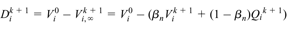
The difference vector $D_j$ decreases which means

$$\sum _{i\in I_k}{\Vert D_{Q_{j,i}^k}^k\Vert }_E\ge \sum _{i\in I_{k+1}}{\Vert D_{Q_{j,i}^{k+1}}^{k+1}\Vert }_E$$

Thus, we have

$$\begin{array}{l}{\Vert D_j^{k+l+1}\Vert }_E={\Vert D_j^{k+l}-[{\beta }_n{D}_j^{k+l}+\frac{1-{\beta }_n}{n}{\displaystyle \sum _{i\in I_{k+l}}{D}_{Q_{j,i}^{k+l}}^{k+l}}]\Vert }_E\\ ={\Vert (1-{\beta }_n)D_j^k-\frac{1}{n}\left[{(1-{\beta }_n)}^{l+1}{\displaystyle \sum _{i\in I_k}{D}_{Q_{j,i}^k}^k}+{(1-{\beta }_n)}^l{\displaystyle \sum _{i\in I_{k+1}}{D}_{Q_{j,i}^{k+1}}^{k+1}}+\cdots +(1-{\beta }_n){\displaystyle \sum _{i\in I_{k+l}}{D}_{Q_{j,i}^{k+l}}^{k+l}}\right]\Vert }_E\end{array}$$

According to the properties of the norm, we get

$${\Vert D_j^{k+l+1}\Vert }_E\le \left|(1-{\beta }_n)\right|{\Vert D_j^k\Vert }_E+\frac{1}{n}\frac{1-{(1-{\beta }_n)}^{l+1}}{1-(1-{\beta }_n)}{\Vert {\displaystyle \sum _{i\in I_k}{D}_{Q_{j,i}^k}^k}\Vert }_E$$

With $0<(1-{\beta }_n)<1$ , we obtain

$$\begin{array}{c}\multicolumn{1}{c}{\Vert D_j^{\infty }{\Vert }_E=\underset{l\to \infty }{lim}\Vert D_j^{k+l}{\Vert }_E\le \underset{l\to \infty }{lim}\{|(1-{\beta }_n)|{\Vert D_j^k\Vert }_E+\frac{1}{n}\frac{1-{(1-{\beta }_n)}^{l+1}}{1-(1-{\beta }_n)}{\Vert \sum _{i\in I_k}{D}_{Q_{j,i}^k}^k\Vert }_E\}}\\ \multicolumn{1}{c}{=(1-{\beta }_n)\Vert D_j^k{\Vert }_E+\frac{1}{n{\beta }_n}\Vert \sum _{i\in I_k}{D}_{Q_{j,i}^k}^k{\Vert }_E}\end{array}$$

which proves the lemma.□

Lemma 1 determines the norm bound of the limit difference vector. Theorem 2 gives the condition to determine whether the active vertex can be fixed or not.

Theorem 2

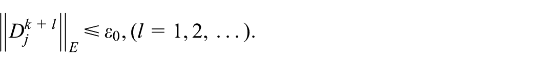
Supposing $V_j$ is the vertex which is active in the lth $(l=0,1,2,\dots ,k-1)$ iteration, which is also the only turn to be fixed in the kth iteration. If the jth difference vector $D_j^k$ satisfies

$$\Vert D_j^k{\Vert }_E\le \frac{{\epsilon }_0}{(1-{\beta }_n)}-\frac{1}{n{\beta }_n(1-{\beta }_n)}\Vert \sum _{i\in I_k}{D}_{Q_{j,i}^k}^k{\Vert }_E$$

(5)

then the vertex $V_j$ will be fixed in the subsequent iterations and $\Vert D_j^l{\Vert }_E$ fulfill

$$\Vert D_j^l{\Vert }_E\le {\epsilon }_0,(l=k+1,k+2,\dots )$$

(6)

where ${\epsilon }_0$ is the pre-defined precision threshold.

Proof

Since $0<(1-{\beta }_n)<1$ , equation (2) is equal to

$$(1-{\beta }_n)\Vert D_j^k{\Vert }_E\le {\epsilon }_0-\frac{1}{n{\beta }_n}\Vert \sum _{i\in I_k}{D}_{Q_{j,i}^k}^k{\Vert }_E$$

Then, we can get

$$(1-{\beta }_n)\Vert D_j^k{\Vert }_E\le {\epsilon }_0-\frac{1}{n}\frac{1-{(1-{\beta }_n)}^l}{1-(1-{\beta }_n)}\Vert \sum _{i\in I_k}{D}_{Q_{j,i}^k}^k{\Vert }_E$$

(7)

With $0<(1-{\beta }_n{)}^l<1,(l=1,2,\dots )$ , we have

$$\Vert D_j^{k+l}{\Vert }_E\le |(1-{\beta }_n)|\Vert D_j^k{\Vert }_E+\frac{1}{n}\frac{1-{(1-{\beta }_n)}^l}{1-(1-{\beta }_n)}\Vert \sum _{i\in I_k}{D}_{Q_{j,i}^k}^k{\Vert }_E$$

(8)

Thus, we have

$$\Vert D_j^{k+l}{\Vert }_E\le {\epsilon }_0,(l=1,2,\dots ).$$

It means that $V_j$ will be fixed in the kth and subsequent iterations if equation (6) holds true.□

Furthermore, we can combine the adaptive data fitting algorithm and the weighted adaptive algorithm. Both the algorithms have advantages.

Adaptive data fitting algorithm and weighted adaptive algorithm

In this section, pseudo-codes of the adaptive data fitting algorithm and weighted adaptive algorithm are given. They are listed as follows.

These two algorithms can be combined during implementation. Applying algorithm 2 to active set in algorithm 1 makes algorithm 1 have better convergence rate and also save a lot of computation. Furthermore, the convergence rate of each vertex can be controlled.

Algorithm 1. Adaptive data fitting algorithm of Loop subdivision surface.

Input: initial control mesh $M^0=\{V_1^0,V_2^0,\dots ,V_n^0\}$ and the given precision ${\epsilon }_0$ . Output: the fitting subdivision surface which satisfies the given precision ${\epsilon }_0$ . Calculate the difference vectors $D_i^0=V_i^0-V_i^{0,\infty }$ ; Let the initial index set be $I_0=\{1,2,\dots ,n\}$ ; Let the active index set be $I=\varnothing$ ; Let iteration times be $k=0$ ; For every element belong to $I_0$ do  if $D_i^k$ is greater than ${\epsilon }_0$ then   i belongs to I;  end end //iterative procedure while I is not empty do  Adjust the active control vertices ${V_i}^{k+1}={V_i}^k+{D_i}^k$ , $i\in I$ ;  Calculate the difference vector $D_i^{k+1}=V_i^{k+1}-V_i^{k+1,\infty }$ , $i\in I$ ;  Classify $D_i^{k+1}$ into two groups: $D_g^{k+1}$ whose norm is greater than ${\epsilon }_0$ , and $D_l^{k+1}$ whose norm is less than ${\epsilon }_0$ ;  Classify $D_l^{k+1}$ into two sets: $D_{\mathrm{s}}^{k+1}$ whose norm satisfies theorem 2, and $D_u^{k+1}$ whose norm does not satisfy theorem 2;  Let the index of $D_g^k\cup D_u^k$ belong to I;   $k=k+1$ ; end

Numerical examples

Algorithm 1: adaptive data fitting algorithm based on the Loop subdivision surface

In this section, six numerical examples are given to compare the computational efficiency of the two different algorithms, namely, normal PI and the adaptive algorithm. For simplicity, we take three basic operations in each iteration as one computational unit. These operations are new vertex generation, vertex evaluation, and difference vector calculation.

Figure 1 is model Bishop. Table 1 shows that normal PI costs 6 iterations to reach the pre-defined precision ${\epsilon }_0={10}^{-1}$ , and all the 250 vertices are adjusted in each iteration during the process. So, normal PI performs $6\times 250=1500$ computational units. The adaptive algorithm takes 7 iterations, but 639 computational units are cost in order to reach ${\epsilon }_0={10}^{-1}$ . The computational units cost by adaptive algorithm is about 43% of normal PI’s.

Figure 1.

Fit model Bishop by the adaptive algorithm, where the initial mesh is displayed in red and the subdivision surface is displayed in yellow: (a) #iter. = 0, #act. = 250; (b) #iter. = 1, #act. = 249; and (c) #iter. = 7, #act.= 3.

Table 1.

Iteration times and precisions of model Bishop.

No. of ${\mathrm{Iter}}_{.}^{\alpha }$	Normal PI		Adaptive algorithm
	No. of ${\mathrm{Act}}_{.}^{\beta }$	Precision	No. of ${\mathrm{Act}}_{.}^{\beta }$	Precision
0	250	2.185	250	2.185
1	250	8.720E−01	249	1.093
2	250	4.749E−01	233	4.999E−01
3	250	2.824E−01	90	2.647E−01
4	250	1.722E−01	17	1.615E−01
5	250	1.063E−01	15	9.891E−02
6	250	6.614E−02	${32}^{\gamma }$	1.369E−01
7			3	6.065E−02

$\alpha$ : iteration time; $\beta$ : number of active vertices; $\gamma$ : new iterative procedure starts with 32 initial active vertices.

Figure 2 is model Ant. Table 2 shows that normal PI costs 5 iterations to reach the pre-defined fitting precision ${\epsilon }_0={10}^{-2}$ , and all the 298 vertices are adjusted in each iteration during the process. So, normal PI performs $5\times 298=1490$ computational units. The adaptive algorithm takes 6 iterations, but 693 computational units are cost in order to reach ${\epsilon }_0={10}^{-2}$ . The computational units cost by adaptive algorithm is about 47% of normal PI’s.

Figure 2.

Fit model Ant by the adaptive algorithm, where the initial mesh is displayed in red and the subdivision surface is displayed in yellow: (a) #iter. = 0, #act. = 298; (b) #iter. = 1, #act. = 266; and (c) #iter. = 6, #act. = 47.

Table 2.

Iteration times and precisions of model Ant.

No. of ${\mathrm{Iter}}_{.}^{\alpha }$	Normal PI		Adaptive algorithm
	No. of ${\mathrm{Act}}_{.}^{\beta }$	Precision	No. of ${\mathrm{Act}}_{.}^{\beta }$	Precision
0	298	6.343E−02	298	6.343E−02
1	298	3.774E−02	266	4.118E−02
2	298	2.406E−02	238	2.268E−02
3	298	1.621E−02	97	1.586E−02
4	298	1.138E−02	42	1.063E−02
5	298	8.245E−03	3	7.161E−03
6	298	6.097E−03	${47}^{\gamma }$	7.921E−03

$\alpha$ : iteration time; $\beta$ : number of active vertices; $\gamma$ : new iterative procedure starts with 47 initial active vertices.

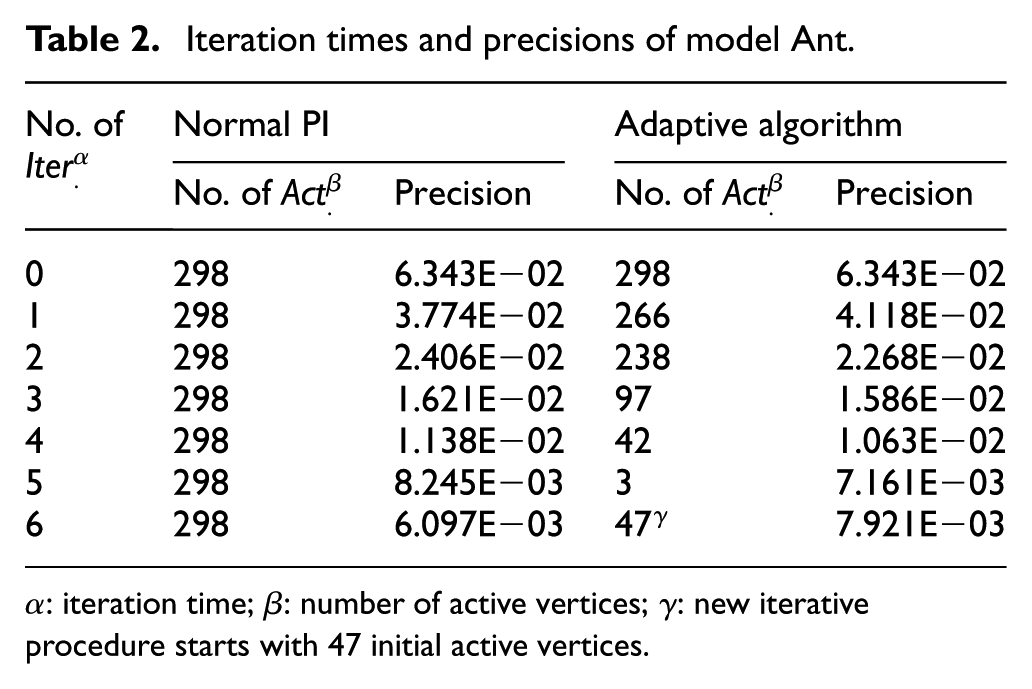
Figure 3 is model Tiger. According to Table 3, normal PI costs 10 iterations to reach the pre-defined fitting precision ${\epsilon }_0={10}^{-2}$ , and all the 2697 vertices are adjusted in each iteration during the process. So, normal PI performs $10\times 2697=26,970$ computational units. The adaptive algorithm takes 11 iterations, but 7453 computational units are cost in order to reach ${\epsilon }_0={10}^{-2}$ . The computational units cost by adaptive algorithm is about 28% of normal PI’s.

Figure 3.

Fit model Tiger by the adaptive algorithm, where the initial mesh is displayed in red and the subdivision surface is displayed in yellow: (a) #iter. = 0, #act. = 2697; (b) #iter. = 1, #act. = 2625; and (c) #iter. = 9, #act. = 817.

Table 3.

Iteration times and precisions of model Tiger.

No. of ${\mathrm{Iter}}_{.}^{\alpha }$	Normal PI		Adaptive algorithm
	No. of ${\mathrm{Act}}_{.}^{\beta }$	Precision	No. of ${\mathrm{Act}}_{.}^{\beta }$	Precision
0	2697	2.494E−01	2697	2.494E−01
1	2697	1.429E−01	2625	1.516E−01
2	2697	9.354E−02	2259	9.065E−02
3	2697	6.467E−02	1217	5.841E−02
4	2697	4.604E−02	392	3.859E−02
5	2697	3.339E−02	93	2.626E−02
6	2697	2.452E−02	26	1.756E−02
7	2697	1.817E−02	4	1.054E−02
8	2697	1.355E−02	1	6.322E−03
9	2697	1.016E−02	${817}^{\gamma }$	2.528E−02
10	2697	7.641E−03	16	1.336E−02
11			3	7.496E−03

$\alpha$ : iteration time; $\beta$ : number of active vertices; $\gamma$ : new iterative procedure starts with 817 initial active vertices.

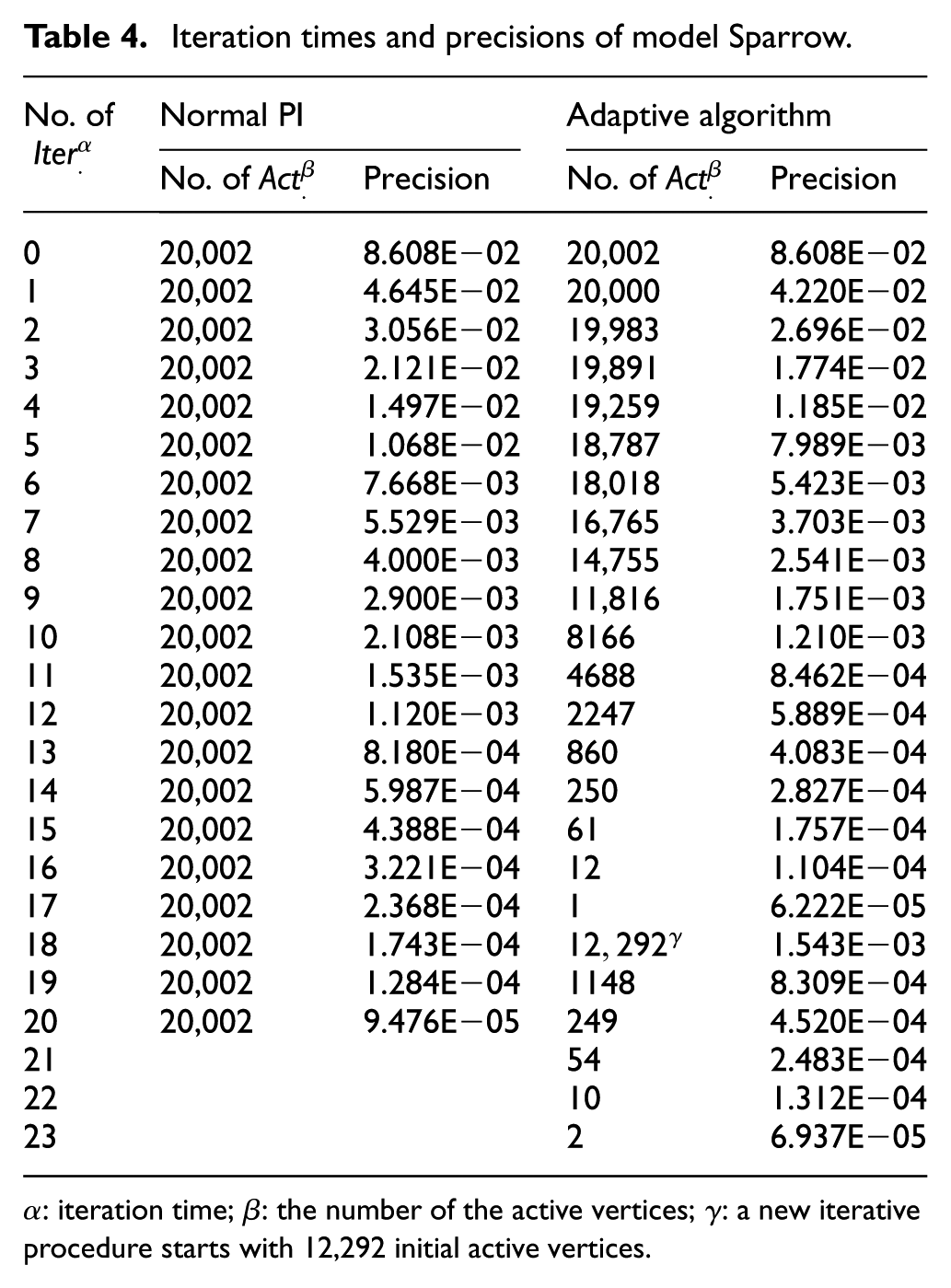
Figure 4 is model Sparrow. Table 4 shows that normal PI costs 20 iterations to reach the pre-defined fitting precision ${\epsilon }_0={10}^{-4}$ , and all the 20,002 vertices are adjusted in each iteration during the process. So, normal PI performs $20\times 20,002=400,040$ computational units. The adaptive algorithm takes 23 iterations, but 189,314 computational units are cost in order to reach ${\epsilon }_0={10}^{-4}$ . The computational units cost by adaptive algorithm is about 47% of normal PI’s.

Figure 4.

Fit model Sparrow by the adaptive algorithm, where the initial mesh is displayed in red and the subdivision surface is displayed in yellow: (a) #iter. = 0, #act.= 20,002; (b) #iter. = 1, #act. = 20,000; and (c) #iter. = 19, #act. = 1148.

Table 4.

Iteration times and precisions of model Sparrow.

No. of ${\mathrm{Iter}}_{.}^{\alpha }$	Normal PI		Adaptive algorithm
	No. of ${\mathrm{Act}}_{.}^{\beta }$	Precision	No. of ${\mathrm{Act}}_{.}^{\beta }$	Precision
0	20,002	8.608E−02	20,002	8.608E−02
1	20,002	4.645E−02	20,000	4.220E−02
2	20,002	3.056E−02	19,983	2.696E−02
3	20,002	2.121E−02	19,891	1.774E−02
4	20,002	1.497E−02	19,259	1.185E−02
5	20,002	1.068E−02	18,787	7.989E−03
6	20,002	7.668E−03	18,018	5.423E−03
7	20,002	5.529E−03	16,765	3.703E−03
8	20,002	4.000E−03	14,755	2.541E−03
9	20,002	2.900E−03	11,816	1.751E−03
10	20,002	2.108E−03	8166	1.210E−03
11	20,002	1.535E−03	4688	8.462E−04
12	20,002	1.120E−03	2247	5.889E−04
13	20,002	8.180E−04	860	4.083E−04
14	20,002	5.987E−04	250	2.827E−04
15	20,002	4.388E−04	61	1.757E−04
16	20,002	3.221E−04	12	1.104E−04
17	20,002	2.368E−04	1	6.222E−05
18	20,002	1.743E−04	$12,{292}^{\gamma }$	1.543E−03
19	20,002	1.284E−04	1148	8.309E−04
20	20,002	9.476E−05	249	4.520E−04
21			54	2.483E−04
22			10	1.312E−04
23			2	6.937E−05

$\alpha$ : iteration time; $\beta$ : the number of the active vertices; $\gamma$ : a new iterative procedure starts with 12,292 initial active vertices.

By comparing the two algorithms (Tables 1–4), the adaptive algorithm is more efficient than the other, costing much less computational units to meet the fitting precision. In general, the adaptive algorithm is especially efficient in fitting large-scale data points, where the fitting precisions of most vertices can reach the pre-defined precision in early iterations, and then the corresponding vertices become fixed. This helps us save a lot of computation.

Algorithm 2: weighted adaptive algorithm for Loop subdivision surface

Table 5 shows the weighted adaptive algorithm of model Tiger, and the given threshold is $a_0=0.1$ .

Algorithm 2. Weighted adaptive algorithm of Loop subdivision surface.

Input: initial control mesh $M^0=\{V_1^0,V_2^0,\dots ,V_n^0\}$ and the giventhreshold $a_0$ .Output: the subdivision surfaces whose vertices satisfy the convergence rate $a_0$ .Calculate the difference vectors $D_i^0=V_i^0-V_i^{0,\infty }$ ;Let the initial index set be $I_0=\{1,2,\dots ,n\}$ ;Let the active index set be $I=\varnothing$ ;Let iteration times be $k=0$ ;For every element belong to $I_0$ do Progressive interpolation to get $M^{k+1}=\{V_1^{k+1},V_2^{k+1},\dots ,V_n^{k+1}\}$ ; Calculate the difference vector $D_i^{k+1}=V_i^{k+1}-V_i^{k+1,\infty }$ , $i\in I_0$ ; Compute the convergence rate ${r_i}^k=\frac{D_i^{k+1}}{D_i^k}$ , $i\in I_0$ ; if ${r_i}^k$ is less than $a_0$ then  i belongs to I; endend//iterative procedurewhile I is not empty do Calculate the weight ${\omega }^{k+1}=\frac{2}{1+\frac{1-r^k}{{\omega }^k}}$ , $r^k=\frac{\sum _{i\in I}{D}_i^{k+1}}{\sum _{i\in I}{D}_i^k}$ ; Adjust the active vertex ${V_i}^{k+2}={V_i}^{k+1}+{\omega }^{k+1}{D_i}^{k+1}$ , $i\in I$ ; Calculate the difference vector $D_i^{k+2}=V_i^{k+2}-V_i^{k+2,\infty }$ , $i\in I$ ; Compute the convergence rate ${r_i}^{k+1}=\frac{D_i^{k+2}}{D_i^{k+1}}$ , $i\in I$ ; Let the index i of $V_i^{k+1}$ , whose difference vector ${r_i}^{k+1}$ is less than $a_0$ , belong to the active index set I;  $k=k+1$ ;end

Table 5.

Iteration times, precisions, and weights of model Tiger.

No. of ${\mathrm{Iter}}_{.}^{\alpha }$	Normal PI	Adaptive algorithm
	Precision	No. of ${\mathrm{Act}}_{.}^{\beta }$	Precision	Weight
0	2.494E−01	2697	2.494E−01
1	1.429E−01	2697	1.429E−01	1
2	9.354E−02	2690	9.354E−02	1.12653
3	6.467E−02	2610	6.103E−02	1.29787
4	4.604E−02	2322	3.854E−02	1.35899
5	3.339E−02	1449	2.457E−02	1.35622
6	2.452E−02	481	1.554E−02	1.3604
7	1.817E−02	136	1.256E−02	1.39444
8	1.355E−02	33	9.459E−03	1.45472
9	1.016E−02	10	6.821E−03	1.49439
10	7.641E−03	4	5.088E−03	1.51594
11	5.766E−03	3	3.831E−03	1.5288
12	4.377E−03	2	2.898E−03	1.53769
13	3.354E−03	2	2.198E−03	1.5441
14	2.573E−03	0	1.670E−03

$\alpha$ : iteration time; $\beta$ : number of weighted vertices.

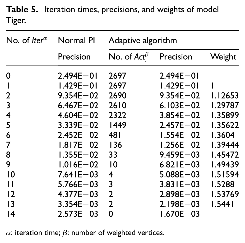
Table 6 shows the weighted adaptive algorithm of model Bishop, and the given threshold is $a_0=0.01$ .

Table 6.

Iteration times, precisions, and weights of model Bishop.

No. of ${\mathrm{Iter}}_{.}^{\alpha }$	Normal PI	Adaptive algorithm
	Precision	No. of ${\mathrm{Act}}_{.}^{\beta }$	Precision	Weight
0	2.185	250	2.185
1	8.720E−01	250	8.720E−01	1
2	4.749E−01	250	4.749E−01	1.07123
3	2.824E−01	250	2.687E−01	1.21819
4	1.722E−01	250	1.416E−01	1.28613
5	1.063E−01	234	7.251E−02	1.28532
6	6.614E−02	217	3.778E−02	1.28133
7	4.145E−02	185	2.003E−02	1.29108
8	2.614E−02	153	1.067E−02	1.30384
9	1.658E−02	89	7.715E−03	1.31529
10	1.057E−02	45	4.529E−03	1.356
11	6.775E−03	9	2.636E−03	1.39002
12	4.359E−03	1	1.653E−03	1.42312
13	2.816E−03	1	1.062E−03	1.43861
14	1.825E−03	0	6.892E−04

$\alpha$ : iteration time; $\beta$ : number of weighted vertices.

Tables 5 and 6 show that the number of weighted vertices decreases with the process of iterations, which means the number of vertices that satisfy the acceleration threshold keeps increasing. The convergence rate of weighted algorithm has been accelerated and the convergence accuracy is higher than that of traditional one.

Conclusion

In this article, one adaptive fitting algorithm for progressive interpolation is developed by the local property of progressive interpolation. The vertices are classified into two dynamic sets, namely, the active set and the fixed set. During the process of iteration, the number of active vertices which needs to be adjusted decreases. Therefore, it helps us save a lot of computation. Weighted adaptive algorithm of progressive interpolation for Loop subdivision surface is also given. The weights have been assigned to the vertices in order to make convergence rate meet the given threshold. Plenty of numerical examples and tables show that subdivision surfaces and data fitting can be effectively applied in data aggregation, data compression, and data fusion.