Sage Journals: Discover world-class research

Abstract

Time-dependent behavior of subcritical crack growth is one of the main characteristics in rocks. The double-torsion test is commonly used to study the slow crack growth behavior of brittle and quasi-brittle materials. However, double-torsion specimen is difficult to processing, the process of the laboratory test is irreversible, and the current numerical simulation is difficult to consider the time-dependent behavior, and so on. In view of all above problems, an idealized particle model was built, and the crack was identified in this article, based on the theory of particle flow. The numerical model was built using Particle Flow Code in 3 Dimensions, and the macromechanical and micromechanical parameters of the model were calibrated. The process of the macroscopic crack propagation and its evolution were analyzed. The intrinsic relations with the load, the displacement, and the time were established. The results show that the Particle Flow Code in 3 Dimensions can reproduce the time-dependent behavior of subcritical crack growth in double-torsion test. And, the peak and the law of the curves are in good agreement with the laboratory test results. Therefore, the Particle Flow Code in 3 Dimensions numerical simulation can be used as a new effective method to reveal the slow crack growth behavior, to get the relevant parameters such as V, K_I, and K_IC, and to build the relationship between V and K_I. The results of this article will have some reference value for the simulation and application of double-torsion test.

Keywords

Double-torsion test subcritical crack growth stress corrosion time-dependent Particle Flow Code in 3 Dimensions

Introduction

The double-torsion (DT) test is commonly used to characterize the slow crack growth behavior of brittle materials. DT specimen was adopted first by Evans¹ and Williams and Evans.² It can be regarded as a symmetrical system of two independent elastic torsions. This test consists in bending one of the edges of a “V” notched plate put on four rollers at each corner (Figure 1). In such setup, one face is loaded in tension whereas the other one is loaded in compression. After a pre-cracking procedure, the DT test can be used for the determination of the fracture toughness or the analysis of slow crack growth. The toughness measurement is conducted at very high loading rate and the record of the maximum load before failure and pre-crack size allows obtaining K_IC. Slow crack growth curves as a function of the mode I stress intensity factor can be measured with a single specimen using different methods: either by a load relaxation test via a compliance calibration curve or by loading the specimen at different loads and measuring the crack growth rates with an optical microscope.

Figure 1.

(a) Specimen shape, (b) cross-section in width, and (c) cross-section in length.

According to the relation between the stress intensity factor and the strain-energy release rate, and the applied load on torsion, and the relation of Poisson’s ratio and shear modulus of the rock, the stress intensity factor can be derived³

K_{I} = \sqrt{Eg} = F W_{m} {[\frac{1 + μ}{η W d^{3} d_{n}}]}^{1 / 2}

(1)

where K_I is the stress intensity factor, N m^−3/2; E is Young’s modulus, Pa; g is the strain-energy release rate, N m⁻¹; F is the applied load, N; W is the width of specimen, m; W_m is the moment arm of the torsion, m; $μ$ is Poisson’s ratio; d is the thickness of specimen, m; $d_{n}$ is the thickness of the specimen along the groove, m (see Figure 1(b)); and $η$ is the corrective factor depending on the ratio $W / d$ (Evans assumed η = 1/3 in 1972).

According to the relation between the compliance of specimen and the length of crack, the relation between the change rate of compliance and subcritical propagation of crack can be set up. Test indicates that the change rate of compliance can be obtained through the change rate of displacement under invariable loads or the change rate of loads under invariable displacement. Under the invariable displacement condition, the subcritical crack velocity of rock equals

v = \frac{da}{dt} = - \frac{W d^{3} Ey}{6 W_{m}^{2} F^{2} (1 + μ)} \frac{dF}{dt}

(2)

where a is the crack length, m; y is the constant displacement imposed on the loading point, m.

Equation (2) shows that if the size of specimen and the displacement on loaded point are known, then the subcritical crack velocity is relate to the load relaxation rate in current loads under the given displacement state. Therefore, we can establish the relation between stress intensity factor K_I and subcritical crack velocity v through the test.

Subcritical crack growth plays an important role in evaluating the long-term stability of structures in rocks. Wu et al.⁴ and Zhao et al.^5–8 carried out a series of theories for crack development. Henry et al.,⁹ Atkinson,¹⁰ and Swanson¹¹ found that the characteristics of subcritical crack growth can be described by a relationship between the stress intensity factor and the crack velocity. At present, the K_I-V relationship and K_IC of rock are measured by the method of constant displacement relaxation of DT specimen. Many scholars^12–15 investigated experimentally subcritical crack growth in granite using the DT test. TY Ko and J Kemeny¹⁶ present the results of studies conducted to validate the constant stress-rate test for determining subcritical crack growth parameters in rocks, compared with the conventional testing method, the DT test. Nara et al.¹⁷ studied the influence of relative humidity on fracture toughness of rock using DT test. P Leplay et al.¹⁸ designed a dedicated experimental setup to perform in situ tests in an X-ray computed tomography scanner on a porous brittle ceramic and to analyze the three-dimensional images with digital volume correlation. Attia et al.¹⁹ investigated the fracture behavior of DT specimens using the finite element method taking no account of the time effect. Zhang²⁰ and Gao and Li²¹ simulated the crack propagation with equivalent cohesive zone method based on virtual internal bond theory. Shyam and Lara-curzio²² summarized the analytical compliance and finite element stress analyses of the DT test specimen. And, they concluded based on the review that standardization of this test method is required in order to make it more practicable.

Beyond its wide use in the literature, the DT test presents some questionings: (1) the brittle rock is processed into an extremely thin plate with a thickness of 3–5 mm, and the process is extremely difficult. (2) The heterogeneity of the rock results in a larger discrepancy. (3) The test loading method is complex and irreversible. (4) Subcritical crack growth is one of the main causes of time-dependent behavior in rocks. The existing numerical simulation results did not involve time.

Fortunately, with the rapid development of numerical calculation method, numerical simulation is solving more and more complex rock mechanics and engineering problems.^23–26 Particle Flow Code in 3 Dimensions (PFC^3D) was established, to research the mechanical characteristic of rock material through the movement and interaction of the particulate media, which is widely used in the study of discontinuous deformation and failure characteristics of rock materials. In this article, based on the theory of particle flow, the command flow of FISH language in PFC^3D will be used to simulate the DT test. And, the feasibility of DT numerical test by PFC^3D will be verified through comparison with indoor experiment.

Crack idealization and identification

Parallel bond behavior

A parallel bond approximates the physical behavior of a cement-like substance lying between and joining the two bonded particles. Parallel bonds establish an elastic interaction between particles that acts in parallel with the slip or contact-bond constitutive models. Parallel bonds can transmit both force and moment between particles, while contact bonds can only transmit force acting at the contact point.

A parallel bond can be envisioned as a set of elastic springs uniformly distributed over either a rectangular (in two-dimensional (2D)) or a circular (in three-dimensional (3D)) cross section lying on the contact plane and centered at the contact point, as shown in Figure 2. These springs act in parallel with the point-contact springs (which come into play when two particles overlap). The behavior of the parallel bond springs is similar to that of a beam whose length, L in Figure 2, approaches zero. Relative motion at the parallel bonded contact (occurring after the parallel bond has been created) causes axial- and shear-directed forces (T and V, respectively) as well as a moment (M) to develop. In PFC^3D, a twisting moment (M_t) may also develop. The maximum normal and shear stresses (σ and τ, respectively) carried by the bonding material can be written as

σ = \frac{T}{A} + \frac{| M | \bar{R}}{I}; τ = \frac{| V |}{A} + \frac{| M_{t} | \bar{R}}{J}

(3)

where A and I are the area and moment of inertia, respectively, of the parallel bond cross section; J is the polar moment of inertia of the parallel bond cross section; and positive T indicates tension.

Figure 2.

Parallel bond idealization (a), forces carried in the 2D bond material (b), and 3D bond material (c).

Crack identification

Microcracks in a PFC^3D synthetic specimen may only form between bonded particles. Particle contact parallel bond model assumes that there is an elastic cementing material between the two particles that connects the two particles together. The relative movement of the contact position results in the bond material generating force and moment.

One mechanism (Cundall et al.²⁷) for the formation of compression-induced cracks is shown in Figure 3(a), in which a group of four circular particles is forced apart by axial load, causing the restraining bond to experience tension. When the tension is large enough, the bond between the particles is destroyed, which indicates the formation of cracks (see Figure 3(b) and (c)). Similar crack inducing mechanisms occur even when different conceptual models for rock microstructure are used. The success of the Particle Flow Code (PFC) material at reproducing the behavior of hard rock can be attributed directly to its ability to generate compression-induced tensile cracks.

Figure 3.

(a) Contact form the parallel bond, (b) the parallel bond is broken, and (c) crack formation.

With the destroyed bond between the particles increasing, the material particles move far away from each other, and their interactions become weaker and weaker, as shown in Figure 4. The bond becomes weaker and weaker. Therefore, under the condition that the displacement loading on the specimen remains constant, the required external forces that keep the cracks continue to grow will become smaller and smaller.

Figure 4.

(a) Prefabricated crack, (b) crack propagation, and (c) crack penetration.

PFC^3D implementation

Geometric model

The model is generated as follows: first, the basic dimensions of the model (150.0 mm × 60.0 mm × 4.80 mm) are defined by the six-sided wall (constrained particle displacement) and then the particles of a given radius are randomly generated within the size range. The total number of particles in this model is 104,138, and the particle radius is Gaussian distribution of R_min ~ R_max. And, in order to reduce the computational complexity and make the show of crack growth more accurate, the block modeling method is adopted in numerical model as shown in Figure 5. Zone 1 is the main zone in which crack will grow, hence the small particles are adopted (R_min = 0.10 mm, R_max = 0.25 mm). Zones 2 and 3 are the zones of little influence, hence the bigger particles are adopted (R_min = 0.02 mm, R_max = 0.40 mm for zone 2, R_min = 0.30 mm, R_max = 0.60 mm for zone 3). The cycle command was written to eliminate the internal non-uniform stress of model, in order to make the model reach to a stable state.

Figure 5.

Calculating model of double-torsion specimen: (a) top view and (b) bottom view.

After generating a stable numerical model, the six confined walls were removed; then, axial groove and V-type notch of specimen were cut by the range and delete command as shown in Figure 5; then, the fix command was used to constrain the bottom displacement at the four corners of the specimen, in order to achieve the purpose of forming point support. Finally, at the top of the model, two square load plates (walls) with a length of 1 mm are defined, and the model is finished.

Model parameter calibration

Micromechanical parameters in PFC^3D are used to characterize the mechanical properties of particles and bonding. Before the numerical model begins to calculate, the micromechanical properties of the model must be given. However, it is difficult to obtain the micromechanical parameters of the model directly from the laboratory test. So, the corresponding parameter calibration is needed.

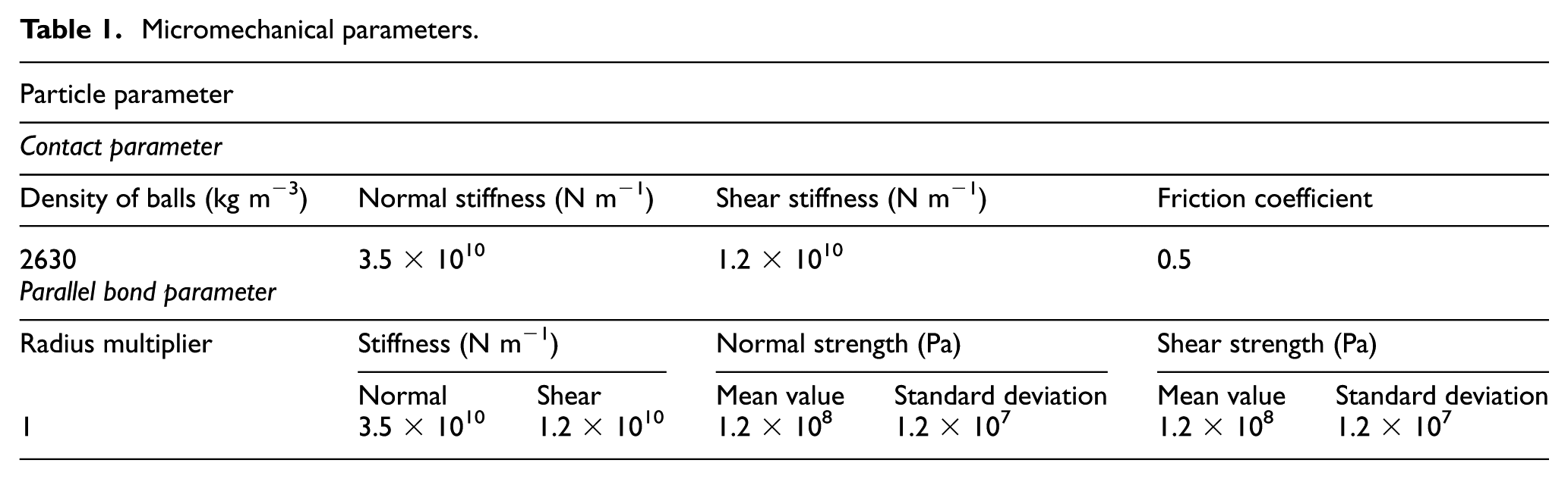
The parallel bond parameters can more reasonably simulate the destruction of brittle rocks by cementing between particles. So, the parallel bond parameters were used in this article. And, the uniaxial compression numerical test was carried out. Comparing with the macromechanical parameters obtained by the laboratory test, the final micromechanical parameters (in Table 1) are obtained by continuously adjusting the numerical parameters in the numerical test, and the results are consistent with the laboratory test and applied to the actual calculation model. The macromechanical parameters from the numerical test, including elastic modulus E, uniaxial compressive strength, and Poisson’s ratio, are similar to those obtained from the laboratory test (Figure 6).

Table 1.

Micromechanical parameters.

Particle parameter
Contact parameter
Density of balls (kg m⁻³)	Normal stiffness (N m⁻¹)		Shear stiffness (N m⁻¹)		Friction coefficient
2630	3.5 × 10¹⁰		1.2 × 10¹⁰		0.5
Parallel bond parameter
Radius multiplier	Stiffness (N m⁻¹)		Normal strength (Pa)		Shear strength (Pa)
	Normal	Shear	Mean value	Standard deviation	Mean value	Standard deviation
1	3.5 × 10¹⁰	1.2 × 10¹⁰	1.2 × 10⁸	1.2 × 10⁷	1.2 × 10⁸	1.2 × 10⁷

Figure 6.

Uniaxial compression curve in numerical simulation.

Loading method

In the laboratory DT test, the four corners of the bottom support platform are set with four steel balls of diameter 5 mm, see Figure 1(a). The specimen is placed on the four steel balls. The front two balls are subjected to the pressure of the loading head, and the tail two pieces only serve to support the specimen. Loading head is also in contact with specimen through two steel balls. The diameter of the two balls is 4 mm. All above steel balls are painted butter. The role of ball bearing support is to ensure the force for the point load, and to reduce the friction between the bearing and the specimen. The test was carried out on an Instron material servo MTS. And, the loading displacement was measured with a high-precision axial extensometer as shown in Figure 7.

Figure 7.

DT test loading system.

Before the DT test is started, the specimen should be pre-cracked. The method is as follows: after the servo loading, head is adjusted to just touch specimen, test starts to load with a constant displacement rate of 0.0008 mm/s.²⁸ And, the loading is recorded at the same time. When the load does not rise with time, pre-crack is completed. At this moment, the loading should be stopped, and the pressure head will be lifted. In PFC^3D, the HISTORY command was used to monitor the loading force. When the loading force does not increase with time, the cracks as shown in Figure 8, appearing on the model, will be thought as pre-crack.

Figure 8.

Loading–time curve of pre-crack.

After the completion of the pre-crack test, the load will be unloaded first, and reloaded to 95% of the pre-crack load.²⁹ Then, the corresponding displacement will be keep as a constant. And, the relaxation test begins. The loading rate is shown in Figure 9. The final displacement of the laboratory test and numerical simulation was 0.2 and 0.215 mm, respectively.

Figure 9.

DT loading displacement–time curve.

The model is applied by the loading plate shown as Figure 5(a). The loading plate is a rigid body, which is brought into contact with the corresponding particles, when the loading plate is pressed against the model at a fixed speed. When the contact occurs, according to the force–displacement law, the contact force will produce between the particles and the wall. Then, according to Newton’s law of motion, the particles will be displaced under contact force, and new contact will occur with the surrounding particles and the walls, resulting in new contact force. This cycle (Figure 10) realizes the loading for the model. And, the force–displacement law can be written as

F_{i}^{n} = K^{n} U^{n} n_{i}

(4)

Δ F_{i}^{s} = - K^{s} Δ U^{s}

(5)

where $F_{i}^{n}$ is the normal force; $K^{n}$ is the normal stiffness; $U^{n}$ is the normal displacement (deformation overlap between particles and particles); $n_{i}$ is the unit normal vector on contact surface; $Δ F_{i}^{s}$ is the increment of shear force; $K^{s}$ is the shear stiffness; and $Δ U^{s}$ is the increment of shear displacement.

Figure 10.

Calculating cycle of model.

The law of motion can be written as

F_{i} = m ({\overset{\cdot\cdot}{x}}_{i} + g_{i})

(6)

M_{i} = {\overset{\cdot}{H}}_{i}

(7)

where $F_{i}$ is the composition of force; m is the particle mass; $g_{i}$ is the acceleration of body force; $M_{i}$ is the resultant moment; and $H_{i}$ is the angular momentum.

Results and discussion

Figure 11 shows the results of the DT laboratory test, and Table 2 shows the details about the DT specimen in this experiments. Figure 12 shows the results of the DT numerical test, in which Figure 12(a) shows the pre-crack diagram and Figure 12(b)–(f) shows simulation of crack propagation diagram from 0.6 to 9 min. Figure 13 shows the crack length–time curve and crack growth velocity–time curve in the DT test with constant displacement relaxation. It can be seen from the figures that the crack propagates along the guide groove in the DT numerical test, and the crack growth velocity gradually decreases as time increases. The phenomenon of crack propagation in the numerical test is consistent with that in the case of laboratory test, which proves that PFC^3D is feasible in simulating DT test and crack propagation.

Figure 11.

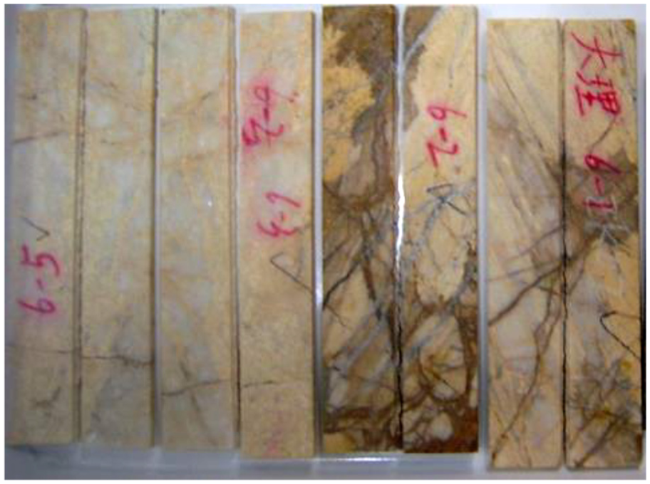
Photo of the damaged specimens in laboratory test.

Table 2.

The property information of double-torsion specimen.

Lithology	Number	L (mm)	W (mm)	d (mm)	D_n (mm)	W_m (mm)	E (GPa)	$μ$
Marble	6-1	180	60.08	4.94	2.42	23.35	26.68	0.24
	6-2	180.38	60.01	5.09	2.78	23.35	26.68	0.24
	6-3	180.05	60.01	5.01	2.54	23.35	26.68	0.24
	6-5	179.96	60.02	5.00	2.48	23.35	26.68	0.24

Figure 12.

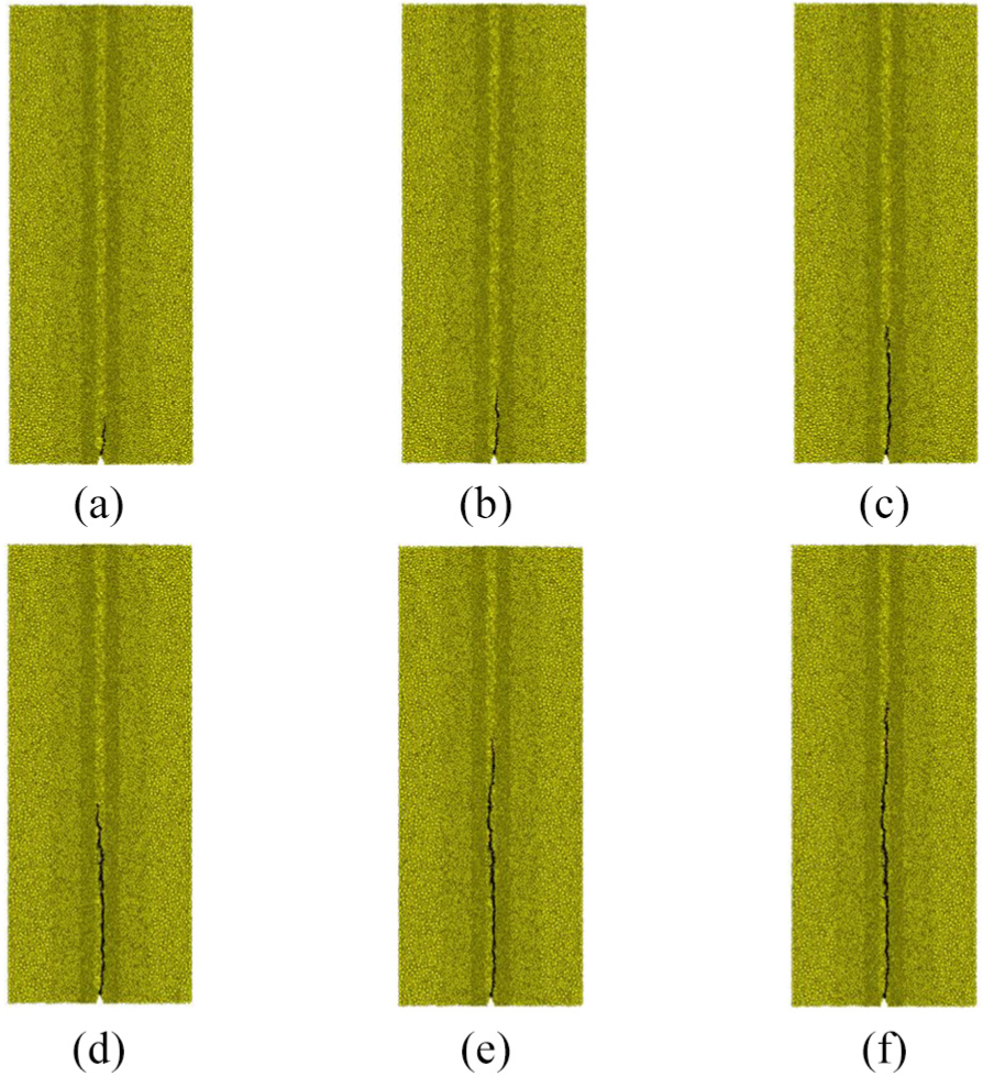
Crack propagation process in the DT numerical test: (a) 0.3 min (pre-crack), (b) 0.6 min, (c) 1.5 min, (d) 3 min, (e) 6 min, and (f) 9 min.

Figure 13.

Crack length–time curve, and crack growth velocity–time curve.

Various engineering examples related to rock mass show that the deformation and failure mechanism of rock mass are closely related to the initiation, propagation, and penetration of cracks in rock mass. The rapid propagation of cracks in rock and the fracture of structure usually occur after the subcritical crack growth to a certain extent, which leads to the time-dependent relationship between the instability of geotechnical engineering and the propagation of cracks in rock.

Figure 14 shows the load–time curve in the DT test with constant displacement relaxation. It is not difficult to find that the load decreases gradually with increase in time and then gradually stabilizes. The peak load of the numerical simulation curve is 165 N, while the laboratory test is 158 N, and the peak difference is 4.2%. The stable load of the numerical simulation curve is 116 N, while the laboratory test is 110 N, and the stable load difference is 5.1%. In the constant displacement relaxation test, the relationship between load and time is in accordance with the following equation

F = a \cdot t^{b} + c = 662.4 \times t^{- 0.0349} - 502.2

(8)

where a, b, c, and I are constants associated with material and loading method.

Figure 14.

Load–time curve in the DT test with constant displacement relaxation.

Compared with the laboratory test results, the numerical simulation is in agreement with the laboratory test results, including the crack propagation law, the displacement–time curve, and the load–time curve. It is shown that the numerical test can better reflect the failure process and the microscopic fracture mechanism of the DT specimen. The reason for the difference between the numerical simulation and the laboratory test may be the mineral composition of the rock, the particle size, and the mechanical properties of the uneven.

We can find from Figure 15 that the curves of lgK_I-lgV can be well linear, but the data measured in the relaxation test keep high discretion. After researching carefully, we think that the high discretion of data is caused by mineral composition, particle size, and mechanical property of the rock itself. In order to reduce the dispersed influence to results, the tests of the same kind of rock should be done many times using the constant-displacement load-relaxation method and return the average values of the regressed coefficients as the characteristic parameters of the subcritical crack of the rock.

Figure 15.

Double logarithmic space lgK_I-lgV.

Conclusion

The DT technique was successfully applied to rock for the study of crack propagation. The technique is able to generate stable crack growth at constant driving displacement. It is suitable for the measurement of fracture characteristics of brittle and quasi-brittle materials, which experience non-linearity due to microcracking in the fracture process zone and crack bridging in the wake.

When the tension is large enough, the bond between the particles is destroyed, which indicates the formation of cracks. Similar crack inducing mechanisms occur even when different conceptual models for rock microstructure are used. The success of the PFC material at reproducing the behavior of hard rock can be attributed directly to its ability to generate compression-induced tensile cracks. With the destroyed bond between the particles increasing, the material particles move far away from each other, and their interactions become weaker and weaker. Therefore, under the condition that the displacement loading on the specimen remains constant, the required external forces that keep the cracks continue to grow will become smaller and smaller.

The PFC^3D can reproduce the time-dependent behavior of subcritical crack growth in DT test. And, the peak and the law of the curves are in good agreement with the laboratory test results. Therefore, PFC^3D numerical simulation can be used as a new and effective method to study the slow crack growth behavior of rock and to get the relevant parameters, such as subcritical crack growth velocity V, stress intensity factor K_I, and fracture toughness K_IC, and to set up the relationship between V and K_I.

Footnotes

Handling Editor: Kenneth Loh

Declaration of conflicting interests

The author(s) declared no potential conflicts of interest with respect to the research, authorship, and/or publication of this article.

Funding

The author(s) disclosed receipt of the following financial support for the research, authorship, and/or publication of this article: This research work was funded by the National Natural Science Foundation of China (51874112 and 51774107); the State Engineering Laboratory of Highway Maintenance Technology, Changsha University of Science and Technology (kfj170108); the Opening Project of State Key Laboratory of Explosion Science and Technology, Beijing Institute of Technology (KFJJ17-12M); the Open Program of State Key Laboratory for Geomechanics and Deep Underground Engineering, China University of Mining and Technology (SKLGDUEK1406); the Open Research Fund of State Key Laboratory of Geomechanics and Geotechnical Engineering, Institute of Rock and Soil Mechanics, Chinese Academy of Sciences (Z013010).

References

Evans

AG.

A simple method for studying slow crack growth in brittle materials. Int J Fracture 1973; 9(3): 267–275.

Williams

Evans

AG.

A simple method for studying slow crack growth. J Test Eval 1973; 1(4): 264–270.

Ciccotti

Gonzato

Mulargia

The double torsion loading configuration for fracture propagation an improved methodology for the load-relaxation at constant displacement. Int J Rock Mech Min Sci 2000; 37(7): 1103–1113.

Chen

Zou

A nonlinear creep damage model for salt rock. Int J Damage Mech. Epub ahead of print 6 August 2018. DOI: 10.1177/1056789518792 649.

Zhao

Wang

et al . Modeling of non-linear rheological behavior of hard rock using triaxial rheological experiment. Int J Rock Mech Min Sci 2017; 93: 66–75.

Zhao

Wang

et al . Transient pulse test and morphological analysis of single rock fractures. Int J Rock Mech Min Sci 2017; 91: 139–154.

Zhao

Zhang

Wang

et al . Cracking and stressstrain behavior of rock-like material containing two flaws under uniaxial compression. Rock Mech Rock Eng 2016; 49(7): 2665–2687.

Zhao

Zhang

Wang

et al . Creep behavior of intact and cracked limestone under multi-level loading and unloading cycles. Rock Mech Rock Eng 2017; 50(6): 1–16.

Henry

Paquet

Tancret

JP.

Experimental study of crack propagation in calcite rocks. Int J Rock Mech Min Sci 1977; 14(2): 85–91.

10.

Atkinson

BK.

Technical note: fracture toughness of Tennessee sandstone and Carrara marble using the double torsion testing method. Int J Rock Mech Min Sci 1979; 16(1): 49–53.

11.

Swanson

PL.

Technical Note: subcritical crack propagation in westerly granite: an investigation into the double torsion method. Int J Rock Mech Min Sci 1981; 18(5): 445–449.

12.

Yuan

Cao

et al . Mechanism study on subcritical crack growth of flabby and intricate ore rock. T Nonferr Metal Soc 2006; 16(3): 723–727.

13.

Nara

Kaneko

Study of subcritical crack growth in andesite using the double torsion test. Int J Rock Mech Min Sci 2005; 42(4): 521–530.

14.

Kaneko

Koike

Yoneda

et al . Relation between subcritical crack growth behavior and crack paths in granite. Int J Rock Mech Min Sci 2006; 43(8): 1256–1261.

15.

Yang

Liu

Zhou

Effects of the loading and unloading conditions on the stress relaxation behavior of pre-cracked granite. Rock Mech Rock Eng 2017; 50(5): 1157–1169.

16.

Kemeny

Determination of the subcritical crack growth parameters in rocks using the constant stress-rate test. Int J Rock Mech Min Sci 2013; 59(5): 166–178.

17.

Nara

Morimoto

Hiroyoshi

et al . Influence of relative humidity on fracture toughness of rock: implications for subcritical crack growth. Int J Solid Struct 2012; 49(18): 2471–2481.

18.

Leplay

Réthoré

Meille

et al . Three-dimensional analysis of an in situ double-torsion test by X-ray computed tomography and digital volume correlation. Exp Mech 2013; 53(7): 1265–1275.

19.

Attia

Mahmoud

Megahed

et al . Numerical investigations of the stepped double torsion fracture toughness specimen. Eng Fract Mech 2010; 77(16): 3359–3367.

20.

Zhang

Numerical simulation of crack propagation with equivalent cohesive zone method based on virtual internal bond theory. Int J Rock Mech Min Sci 2009; 46(2): 307–314.

21.

Gao

Modeling fracture in nanomaterials via a virtual internal bond method. Eng Fract Mech 2003; 70(14): 1777–1791.

22.

Shyam

Lara-curzio

The double-torsion testing technique for determination of fracture toughness and slow crack growth behavior of materials: a review. J Mater Sci 2006; 41(13): 4093–4104.

23.

Zhao

Luo

Wang

et al . Numerical analysis of Karst water inrush and a criterion for establishing the width of water-resistant rock pillars. Mine Water Environ 2017; 36(4): 508–519.

24.

Hua

Nie

Cai

et al . Pattern characterization concerning spatial and temporal evolution of dust pollution associated with two typical ventilation methods at fully mechanized excavation faces in rock tunnels. Powder Technol 2018; 334: 117–131.

25.

Wang

Guo

Dai

et al . Behaviour and modelling of fiber reinforced clay under triaxial compression by using the combining superposition method with the energy based homogenization technique. Int J Geomech 2018; 18(12): 04018172.

26.

Wang

Guo

Ren

et al . Laboratory investigation on strength characteristics of expansive soil treated with jute fiber reinforcement. Int J Geomech 2017; 17(11): 04017101

27.

Cundall

Potyondy

Lee

. Micromechanics-based models for fracture and breakout around the mine-by tunnel. In: Martino

Martin

(eds) Proceedings of the excavation Ýsturbed Zone Workshop, designing the excavation disturbed zone for a nuclear repository in hard rock. Toronto: Canadian Nuclear Society, 1996, pp.113–122.

28.

Yuan

Cao

Zhou

ZY.

Testing study of subcritical crack growth of ore in Jinchuan mine. J Central South Univ: Sci Technol 2006; 37(2): 381–384.

29.

Ciccotti

Negri

Sassi

et al . Elastic and fracture parameters of Etna, Stromboli, and Vulcano lava rocks. J Volcanol Geoth Res 2000; 98(1): 209–217.

Time-dependent behavior of subcritical crack growth for rock plate: Experimental and numerical study

Abstract

Keywords

Introduction

Crack idealization and identification

Parallel bond behavior

Crack identification

PFC3D implementation

Geometric model

Model parameter calibration

Loading method

Results and discussion

Conclusion

Footnotes

Declaration of conflicting interests

Funding

References

PFC^3D implementation