Sage Journals: Discover world-class research

Abstract

This article introduces a time-selective strategy for enhancing temporal consistency of input data for multi-sensor data fusion for in-network data processing in ad hoc wireless sensor networks. Detecting and handling complex time-variable (real-time) situations require methodical consideration of temporal aspects, especially in ad hoc wireless sensor network with distributed asynchronous and autonomous nodes. For example, assigning processing intervals of network nodes, defining validity and simultaneity requirements for data items, determining the size of memory required for buffering the data streams produced by ad hoc nodes and other relevant aspects. The data streams produced periodically and sometimes intermittently by sensor nodes arrive to the fusion nodes with variable delays, which results in sporadic temporal order of inputs. Using data from individual nodes in the order of arrival (i.e. freshest data first) does not, in all cases, yield the optimal results in terms of data temporal consistency and fusion accuracy. We propose time-selective data fusion strategy, which combines temporal alignment, temporal constraints and a method for computing delay of sensor readings, to allow fusion node to select the temporally compatible data from received streams. A real-world experiment (moving vehicles in urban environment) for validation of the strategy demonstrates significant improvement of the accuracy of fusion results.

Keywords

Time-selective data fusion in-network data processing data validity data alignment data simultaneity wireless ad hoc sensor networks situation awareness middleware

Introduction

Detecting complex situations in real time typically requires simultaneous observations originating from several autonomous and multi-modal wireless sensor network (WSN) nodes. The problem, however, when employing ad hoc WSNs, is that the data transport times of even simultaneous sensor readings, acquired by distributed nodes, may not match temporarily even if the same communication path is used. This article focuses on communication between sensor and fusion processes, explores how readings from multiple distributed sensor nodes are consumed by the fusion node in real time and how data validity and simultaneity intervals affect the selection of temporally matching data for fusion process.

The purpose of the information produced by the WSN nodes at the edge of the network is to cater for the needs of the data users¹ deeper in the WSN. When used for situation awareness (SA) applications, the credibility of such information depends on timely processing of sensor data within the network and the temporal validity of data used.^2,3 The users subscribe to situational information of interest, not from a central server but directly from nodes performing in-network data processing,⁴ which are able to provide the requested SA information. The in-network processing nodes in turn subscribe to data from sensor nodes. The subscription contains information about what data should be provided, its expected refresh rate and can also specify the requirements for validity and simultaneity intervals. The WSN middleware for handling the subscriptions for exchanging SA information has been introduced in our previous work.⁵

In this article, we consider the communication between asynchronous WSN nodes – meaning that clocks in different nodes are not synchronized and the start-up, data production and consumption processes in the nodes are activated independently from each other. The nodes in the network may employ different operating modes or duty cycling schemes and incorporate several heterogeneous sensors, with different modalities, characteristics and sampling frequencies. When a sensor node receives a subscription, it activates a periodic or event-based process for data production, the parameters of the process being dependent on the details of the subscription. Each WSN node may simultaneously service multiple active subscriptions and respectively run several processes for data production or consumption. The data produced by periodic execution of sensor processes (as subscribed by fusion processes) form data streams which can be intermittent⁴ with elements not uniformly distributed in time with the possibility of some elements being sporadically delayed due to behavioural pattern of ad hoc WSN. As a result, some of the stream data elements may violate the required validity periods,³ arrive out of order^6,7 and can often have only partial temporal coverage.⁸ This behaviour could be caused by several factors, such as the combined effect from the application of low data rate communication standard (e.g. IEEE 802.15.4, Bluetooth Low Energy or proprietary standards), ad hoc nature of WSN and an unpredictable, volatile – that is, disconnected, intermittent and low-bandwidth (DIL) – communication environment,⁹ where WSN nodes operate. Therefore, the sensor readings used in the order of arrival as inputs for in-network data fusion and aggregation processes may not characterize the same situation. Hence, using always the freshest data from available streams may not be desirable. We suggest that only temporally and spatially compatible data should be fused and/or combined to infer new synthesized readings, and we propose a strategy for selection of temporally suitable data for improving the temporal consistency of input data for in-network processing. The strategy, implemented in the WSN fusion nodes’ middleware component as a default service, combines the use of temporal constraints⁴ with a temporal alignment and selection algorithm and is customized for processing multiple streams of sensor data, which can be intermittent and arrive out of order. The mechanisms for data alignment, selection of suitable input data and verifying them against validity and simultaneity constraints are described using Q-modelling formalism.¹⁰ Q-model allows to model the data streams in distributed systems (e.g. WSNs) and to analyse the delays of stream elements caused by periodic or sporadic activations of asynchronous processes in distributed systems (e.g. WSN nodes). As opposed to other methods that use time constraints and prefer freshest data first for time-sensitive WSN applications, the time-selective strategy allows fusion node to purposefully select temporally compatible data items from input streams.

An urban traffic monitoring experiment is used to demonstrate the enhancement of temporal consistency of input data for in-network data processing and a respective significant improvement in accuracy of data fusion results.

Section ‘Related work’ gives a short overview of the related work. Section ‘Modelling data streams and time-selective data fusion in WSN’ describes dataflows in ad hoc WSN using Q-model formalism, explains important theoretical notions to avoid ambiguity and introduces the alignment and selection algorithm. Section ‘Accumulated delays of the sensor readings’ describes the method for delay computation for the sensor readings and explains why it is necessary. Section ‘Experiment setup’ describes the experiment setup. Section ‘Results’ describes the results of the field tests, analysing the influence of time-selective strategy on in-network data processing, and section ‘Conclusion’ concludes this article and discusses some relevant aspects and future directions.

Related work

Timely handling of SA information collected by WSN requires distributed data fusion and aggregation by network nodes within the network. Instead of transporting all sensor data to a central server, we apply the paradigms of edge computation and in-network data processing.⁴ The former is about performing as much computation close to the source of data as possible (either in sensor nodes or close to them) and the latter is about completing data fusion and aggregation within the network to mitigate bandwidth and energy scarcity, to increase solution resilience and the reliability of situation detection.

In most WSNs, the data acquired by sensors are processed in the same order as they arrive – even if the overall structure of the network and the definitions for detectable situations are known at design time. For example, Izadi et al.¹¹ present a data fusion approach which distinguishes low-quality input data from good-quality input data by assigning weights on sensor readings. The network delay is considered as one of the factors in the computation of weights, such that sensor readings with longer delays have lower influence on fusion result. This approach favours the freshest data and discards the opportunity to use delayed data that may be of high quality and better suitable for multi-sensor fusion. Other examples of prioritizing data freshness can be found in the papers that analyse quality-of-service (QoS) aspects in WSNs. A good survey of the state-of-the-art QoS techniques for delay handling and reliability mechanisms is provided in Al-Anbagi et al.¹² Similar overviews of WSN solutions for manufacturing and industrial control are given by Zhao¹³ and Diallo et al.³ The solutions described have reasonably good time-aware behaviour, that is, the ability to handle time-critical data and time-sensitive communication. However, the QoS aspects, such as real-time constraints and data freshness are considered most important in these surveys.

Another approach to guaranteeing timeliness in conventional WSN systems is to design them so that the delays caused by different communication paths meet the given deadlines.¹⁴ Such strategy cannot cater for asynchronous nature of DIL and ad hoc WSN, where in-network data processing occurs with random and intermittent data bursts. Cheng et al.¹⁵ present a method to modify the network structure in order to optimize the delays and to minimize the energy consumption. However, the structure of ad hoc networks is difficult to control by nature, hence the method suggested in Cheng et al.¹⁵ may not applicable here. In order to provide better understanding of timeliness capabilities of WSNs,^16,17 consider probabilistic methods for traffic flow aspects, such as end-to-end delay, jitter and throughput. Both works point out that in most practical cases, the worst-case bounds for end-to-end delay in WSNs are not applicable. We emphasize that in ad hoc sensor networks and especially in networks for collecting SA information, the data consumer must be able to analyse the validity of the data online¹⁸ and to determine how long the data are usable. The time-selective strategy for in-network processing can handle more variability in end-to-end delays, but requires a means to compute the delays accumulated during the data transport through the network.

The main sources for timing non-determinism in contemporary WSNs include transmission delays, packet losses, queuing for transmission, nodes contest for radio frequency medium and clock drifts and jitters in individual nodes of the network. Transmission-related delays originating from send time, access time, propagation time and receive time are a well-researched area in traditional Ethernet-based networks.¹⁹ In ad hoc WSN solutions, where time synchronization is not used, the transmission related non-determinism can be mitigated for low number of hops by applying contemporary transceivers (e.g. using IEEE 802.15.4 protocol), which allow for modifying the contents of a packet after packet transmission is started by utilizing delay computation method described in Maroti and Sallai.²⁰

Timing challenges in WSNs also include packet losses, which can happen due to dynamically changing network structure and unreliable wireless links.¹² The nodes may autonomously join or leave the network, interference from other sources may influence the wireless links (which may force the WSN to find different routing paths) and also mobile nodes must be considered. The delays can arise also from interactions where sending node is unable to transmit due to periodic activation, low duty cycle or other network scheduling policies, the resulting queuing delays for partner nodes are often ignored. Although the execution periods of the processes in network nodes may be highly deterministic, the messages are delayed and transmitted at non-deterministic times. This causes the end-to-end delays to be highly unpredictable, and the same applies to the order of data elements as packets may arrive out of order. Each time the system’s structure changes due to changing goals by users or the environment, the network must adapt to the changing interaction patterns and delays.

Another aspect complicating timing analysis in an ad hoc WSN is unpredictability of the data production by autonomous nodes. First, the traffic rates of produced data by sensor nodes depend on the application, sensor modalities and sensor process signal processing capabilities. For example, more intelligent and autonomous sensor nodes can avoid reporting altogether if the monitored situation is unchanged or report only as often as required by the rate of change of situation (i.e. monitoring environmental aspects may not need as high rate of reports as measuring current or voltage spikes, or tracking a mobile object). Second, nodes in WSN often apply duty cycling or other transmission scheduling policies to mitigate bandwidth and energy usage.²¹ Doing these decisions autonomously according the current situation, regarding environment or local energy level adds unpredictability.

The problem of handling out-of-order data for sensor fusion is not well researched in scientific literature²² and even less so in papers considering ad hoc WSNs. In area of multi-sensor data fusion, the related topic is called out-of-sequence measurements (OOSM).²² OOSM can be caused by variable propagation times for different data sources or by heterogeneous sensors operating at multiple rates. The problem becomes especially relevant in large-scale networks consisting hundreds to thousands of measuring devices, as the complexity of network communication increases and communication delays of data packages get bigger.²³ In the area of multi-sensor data fusion, the solutions for this problem focus mostly on enhancing filtering algorithms (e.g. Kalman filter or particle filter) that cope with measurements arriving only a single or a few steps later.^22,24 We consider those approaches not well suited for in-network multi-sensor fusion in ad hoc WSNs. The delays in such networks can be much more unpredictable and longer and approaches considering filtering and state estimation are computationally more complicated and resource demanding.²³ Some early examples that consider out-of-order arrival of data for in-network processing in WSNs are Shi et al.²⁵ and Xiaoliang et al.²⁶ While both papers consider OOSM filtering approach with discrete step delays, the former handles mixed and bounded delays from a single sensor and the latter deals with delays from multiple sensors with delay length of a single sensor data refreshing period. These approaches are still in their early stages and not yet suitable for DIL and ad hoc WSNs where multi-sensor fusion is considered.

A good overview of the existing data fusion techniques for WSN is given by Yadav et al.,²⁷ but the listed works in given overview neither consider variable arrival delays in ad hoc networks or streams that may result in out-of-order arrival to the fusion node nor give sufficient attention to other timing characteristics other than freshness of data. Examples of distributed data fusion in WSNs are described in Bahrepour et al.²⁸ and Lai et al.,²⁹ where events detected and sensor readings collected by individual sensor nodes are assembled by a fusion node. These works do not discuss the validity or simultaneity of the input data for the fusion algorithms.

Classical models for distributed systems often use abstractions at various levels to compensate for timing non-determinism.³⁰ Examples are lock-step synchronous models,³¹ fixed or no drift in individual clocks³² and/or delays with fixed bounds³³ (which essentially models a subset of synchronous systems). We consider the Q-modelling technique³⁴ for the analysis of ad hoc WSNs, as it naturally facilitates modelling of timing aspects of asynchronous communication and queuing delays across the communication paths through the network while considering the precision of data timestamps. The original purpose of the Q-model is to analyse time correctness of interprocess communication of a collection of loosely coupled, repeatedly activated and terminating processes,¹⁰ where the purpose of the time-selective communication is that the input data for the consumer process should be exact from the desired time interval (not produced before or after that time interval – the freshest data are not always desirable). However, the time-selective communication on such autonomous and distributed real-time systems results in a situation where some of the execution sequences and data produced by them are discarded and some may be used as inputs to another process several times.³⁴

Modelling data streams and time-selective data fusion in WSN

This section defines and explains some important concepts, such as temporal alignment of data, validity time of a stream element and simultaneity interval for stream elements across streams from different sources. The section also introduces a time-selective data fusion strategy for WSN and gives a detailed overview of the algorithm for the temporal alignment of data and selection of compatible elements for data fusion.

Sensor readings arriving out of order

In order to illustrate the necessity for selecting temporally correct data from sensor data streams for data fusion, we describe a simple freezer example. Imagine a large freezer which has several spatially distributed temperature sensors inside. As using wired sensors in such an environment can be costly and difficult to deploy, WSN technology is used for convenience. All wireless nodes are considered asynchronous, that is, each node has its own individual clock that is not synchronized to the global reference. In this example, only the latest readings from each of sensors are fused to get an average. The fused value is reported to the user periodically. Neither sensor readings nor fusion results are stored in the fusion node. If the temperature rises equal or above zero, there is a risk of spoiled goods. The notion of data fusion in this example is an exaggeration and is used for consistency reasons. The example is illustrated in Figure 1. The white round markings on sensors time axis indicate sensor readings with normal delay. The black round markings indicate sensor readings with increased delay, and dashed line indicates the delay as it was expected by the designer of fusion algorithm. The computation and reporting of the averaged results take place at instances indicated by the ticks on fusion time axis.

Figure 1.

Example with delayed sensor readings causing out-of-order arrival.

The cause for the increased delay, as depicted in Figure 1, could be a route change in the multi-hop network as goods are being stacked up on the radio path (similar increased delay could easily be caused also by network overload, etc.). Consider a situation where both sensors register a 0° value, but due to changed route, one of the sensor readings delay increases (now another WSN node relays its readings to the fusion node). If the fusion node does not consider variable delays and averages only readings according to their arrival, then the reported temperature never rises above −1.0° and the fact that the freezer temperature was zero for a short period of time is left unnoticed. It should be noted that even if there are no increased delays in the described freezer example, there is still a chance that the zero temperature would not be reported. As processes in this example are considered asynchronous, the fusion node execution and following reporting can happen between the arrival of two zero readings.

To mitigate such problems, we present a time-selective strategy. The fusion node should, during each of its algorithm execution, have access not only to the latest sensor readings but also preferably to an array or a batch of past readings from each distributed sensor. The storage size for the available past readings should be large enough to hold also readings as old as the longest allowed delay that can happen for fusion inputs for that particular network. Furthermore, it should be possible to align the arrived readings from different sensors to the fusion node’s time axis. This makes it possible for fusion process to select readings that are compatible in the temporal domain. The theoretical model for time-selective data fusion is discussed and analysed in the next section.

Modelling time-selective data fusion in WSN

We use Q-model¹⁰ formalism to specify and model the WSN as a distributed communication system, consisting two main classes of components: processes and channels. Each interacting node in the WSN can execute several different processes p. The communication between the processes in different nodes across the WSN is modelled by a channel $σ_{sf}$ , where s denotes a sensor process and f denotes a data fusion process, respectively, that are communicating. The channel is a logical tool that maps the output from one process to input of another process according to their timesets with the expression

σ_{sf} : T (p_{s}) \times T (p_{f}) \times val p_{s} \to pro j_{val p_{s}} dom p_{f}

which, in the context of this article, conveys sensor process values to fusion process domain of definition. Here, the sensor process $p_{s}$ and fusion process $p_{f}$ are considered to be running, respectively, in disparate network nodes for sensing and fusion (in some scenarios, it is also possible that a single network node is running both processes). The variables $T (p_{s})$ and $T (p_{f})$ represent the execution timesets of these processes. The mappings between processes are activated repeatedly, either periodically or sporadically. For example, the execution timesets for periodically activated processes can be modelled by expression

T (p) = {t : t_{n} = t_{0} + n \cdot t_{a}}

where $t_{0} = 0$ , $n \in N$ and $t_{a}$ is the interval between two process executions. The processes are considered asynchronous and have each their own timeset and time counting mechanism. For modelling purposes, each activation/execution instant $t_{n}$ for a process also determines the timestamp of the data produced by this process. When the produced data is transmitted by the node, its timestamp is updated to reflect the delay between the process activation instant and the actual transmission moment. The practical process of delay computation is described in section ‘Accumulated delays of the sensor readings’. If computationally feasible, the timestamp is also updated to reflect the actual time-moment of the physical-world situation that is captured by sensor process. Computing the exact time instant of the situation might not always be trivial due to limited resources of low-cost WSN nodes.

The data usage between processes is time-selective. The data stream resulting from data produced by one of the processes is moderated by the channel function and transferred to another process. Formally, the channel function is expressed as

K (σ_{sf}, t) \subset T (p_{s}), t \subseteq T (p_{f})

where the number of stream elements conveyed by channel or rather temporal span of the accessible elements received by fusion process is defined as time interval $K (σ_{sf}, t) = [μ, ν]$ on the time axis of the fusion process. An overview of the nodes, processes and related channels is given in Figure 2. Each node may run several processes, where each process may have its own execution timeset and execution period. Each sensor process execution can result in a sensor reading which is conveyed to the fusion process via the channel function. Each fusion process (data consumer) establishes a separate channel for each sensor (data producer) process. Each channel may have a different interval $[μ, ν]$ of the accessible elements, and the fusion process has access to the transmitted sensor readings according to the channel function.

Figure 2.

Overview of processes and channels.

For example, for the fusion process $p_{f}$ during its single execution, the interval $[μ, ν]$ represents the requirement for the accessible stream elements from sensor process $p_{s}$ . The variables $μ$ and $ν$ are defined by the fusion process and represent, respectively, the earliest (oldest) and latest (freshest) instants of the sensor process output data. Usually, $ν = 0$ as the freshest possible data is required by the fusion process. During each execution, the fusion process can read data from several channels, that is, it can have access to several streams, each from a different process. The actual time instant for the freshest possible element for specific channel for the interval $[μ, ν]$ is specified by the expression

t = \max_{t_{s}} {t_{s} < t_{f} + η (σ_{sf}, t_{f}) - ζ (p_{s}, t_{s})}

where $t_{s} \subseteq T (p_{s})$ , $t_{f} \subseteq T (p_{f})$ , and $η (σ_{sf}, t_{f})$ is the length of time interval during which the fusion process receives the data. The variable $ζ (p_{s}, t_{s})$ computes the execution time of the sensor process. For simplicity, the propagation time of a radio packet is considered zero. The actual delay due to periodic execution of processes at any fusion execution instant can be computed by the formula

φ_{n} (t) = t_{f} - t_{s}

The oldest feasible element (denoted with variable $μ$ ) for each channel during a single fusion process execution is determined according acceptable delays according to the use case or the estimated delays from other streams used for same fusion process. As a consistent stream of data elements must be stored, the oldest feasible element stored is practically limited by the maximum number of elements stored, which is limited by the memory available on the node.

Regarding the feasibility of alignment and selection of temporally suitable sensor readings for fusion process, the memory buffers for storing the sensor readings from different channels should be large enough to cope with the delays caused by the nature of ad hoc DIL WSN.

Temporal validity interval of input data

This section discusses the importance of temporal validity intervals of input data for fusion node and how the value of validity interval of sensor readings affects the selection of temporally compatible inputs for the data fusion in WSN. The necessity of checking and ensuring the sensor data validity has been discussed in our earlier papers,^4,35 where it has been explained how every sensor reading has temporal and spatial validity intervals associated with it. These intervals depend on several aspects, for example, the validity area depends on the location of the WSN and on the properties of the phenomenon being observed, while the temporal validity interval depends both on the properties of the environment where the node is located and on the phenomenon being observed. The sensor node augments its output data, with the validity intervals, and verifies that readings are still valid before transmitting them. The fusion node in turn verifies that the validity intervals of the sensor readings upon their arrival do match with the constraints set on incoming data. The output of the fusion process is in turn again accompanied with the metadata which also contains respective validity intervals checked by the users of fused data.

It is difficult to determine the precise arrival time of data to the fusion node in an ad hoc WSN in advance. The temporal validity interval is used to set an upper bound on the transport and usability time of the sensor readings. When temporal validity interval expires before the sensor readings arrive to the fusion node, the readings are discarded. The temporal constraints employed by the fusion node are not necessarily related to the validity intervals of arriving data. The constraints can be stricter or more relaxed depending on the application and context (as decided online by the fusion node or at design time by the system designer). If the validity of arrived data satisfies the temporal constraints, it is stored in the fusion node memory, where it remains available so that the fusion process can select the suitable inputs at the right time. Figure 3 describes a timestamp and a validity interval for a sensor reading on a fusion node timeline. The timestamp $t_{s}$ indicates the time moment when the sensor reading was acquired and the validity interval $I_{validity}$ indicates the period of time during which the resulting sensor reading is valid.

Figure 3.

Timestamp and a validity interval.

The validity interval for a single sensor reading with timestamp $t_{s}$ can be expressed as follows

I_{validity} = [t_{s}, t_{s} + t_{valid}]

where $t_{valid}$ is a length of validity interval on fusion node’s time axis.³⁵ In case the fusion node receives input data from different sources, all the data must be valid at their arrival.

Fusion requires overlapping validity of stream elements

Validity intervals of individual data elements can be used for grouping data and selecting data elements with overlapping validity intervals. Figure 4 depicts four sensor readings, their timestamps and validity intervals. The $t_{S 1}$ , $t_{S 2}$ , $t_{S 3}$ and $t_{S 4}$ are the timestamps of the sensor readings aligned on the fusion node time axis, and black rectangles indicate the respective validity intervals $I_{valid} (t_{Sn})$ . It can be observed that sensor reading with timestamp $t_{S 2}$ falls within the validity interval of another sensor reading with timestamp $t_{S 1}$ . There is a period of time during which both sensor readings are valid and both can be used as inputs for fusion process. This period of simultaneous validity or an overlapping validity interval can be expressed as

I_{valid} (t_{S 1}, t_{S 2}) = I_{valid} (t_{S 1}) \cap I_{valid} (t_{S 2})

The opposite situation can be observed in case of $t_{S 3}$ and $t_{S 4}$ , where the validity of sensor reading with timestamp $t_{S 4}$ does not overlap with the validity of sensor reading with timestamp $t_{S 3}$ , thus they should not be used together for detection or synthesis of a more abstract situation (i.e. data fusion). Supposing now that there are several distributed sensors that produce data streams, the fusion will provide correct results only when the fusion process takes as an input, sensor readings that are valid simultaneously, that is, for which there exists a common overlapping validity interval. However, one can also consider a situation where the fusion process, after its execution, has access to data which were valid during their arrival at fusion node, but which validity has expired by the time moment when the actual selection of suitable input data takes place (the channel length of accessible input data for fusion may be longer to hold also data, which validity has expired). In this case, it is important that the validity intervals of potential input data from different sources have an overlap. The resulting fusion output data have their own validity interval assigned before the fusion output is transmitted to its corresponding consumer. The validity interval of fusion output is subjected to same constraints as described previously.

Figure 4.

Overlap of validity intervals.

The feasibility analysis of fusion of stream elements requires us to consider some necessary design decisions – for example, assigning periodicity of sensor reading, defining validity intervals for sensor readings, managing clock jitter in sensor nodes, maintaining average traffic speed between network nodes and defining the length of simultaneity interval that enables data fusion.

Simultaneity interval

The simultaneity interval serves a dual role – it enables to convey and evaluate the actually achieved synchronicity in a network and, if necessary, to compare it with the required synchronicity; and it provides a design parameter for assigning validity intervals for individual sensor readings in order to achieve feasible fusion of those readings. In general, the simultaneity interval specifies a set of events (e.g. sensor readings) that can be considered ‘simultaneous’ within some window of tolerance and can be used for fusion, and it is a period of time that elapses from the occurrence of the first of a group of events until the occurrence of the last event of the same group.¹⁰ A simultaneity interval for two sensor readings with timestamps $t_{S 1}$ and $t_{S 2}$ is expressed as

I_{sim} (t_{S 1,} t_{S 2}) = | t_{S 2} - t_{S 1} |

For example, if fusion process receives four sensor readings as inputs with the delays of $d_{1} = 980 ms$ , $d_{2} = 1010 ms$ , $d_{3} = 875 ms$ and $d_{4} = 1045 ms$ , the simultaneity interval for these inputs is $I_{sim} (d_{1}, d_{2}, d_{3}, d_{4}) = 170 ms$ .

As design goal or rather a requirement for simultaneity of sensor readings (more precisely the observed situations that the sensor readings represent), we define the simultaneity constraint $C_{sim}$ . For example, if we look at the two sensor readings with timestamps $t_{S 1}$ and $t_{S 2}$ depicted in Figure 4, the correct fusion of these readings requires (in addition to overlapping validity intervals) that the simultaneity interval of the given group of sensor readings satisfies: $C_{sim} \geq I_{sim}$ . This requirement is independent of the group size, all sensor readings grouped into single $I_{sim}$ according to their timestamps must satisfy $C_{sim}$ in order to be interpreted as simultaneous.

In practice, the simultaneity constraint is first chosen on the basis of application and second on the basis of the precision of computed delays of sensor readings. The computation of delay of sensor readings is discussed in section ‘Accumulated delays of the sensor readings’. The sample application used in this article is the detection of moving vehicles. The choice of simultaneity constraint will influence the precision of the position estimate of the detected vehicle. For example, if $C_{sim} = 400 ms$ is chosen, the position of the vehicle is interpreted to be within the area it can cover in 400 ms (given that the speed of the vehicle is known).

Alignment and selection of compatible elementsfrom streams

The basic idea of the alignment and selection algorithm is to group the available readings from different sensors by temporal characteristics (such as validity intervals $I_{validity}$ and/or simultaneity interval $I_{sim}$ ) and to use only these groups as inputs for fusion process. The need for such an approach is driven by the problem which arises when distributed and autonomous ad hoc WSN nodes are used for simultaneous observation to detect complex situations in real time. Due to the delays, the sensor readings used as inputs for in-network distributed fusion and aggregation nodes may not characterize the same real-world situation if used in the order of arrival. One of the real-world cases can be observed in Figure 10, where the received stream elements have been projected onto the fusion node’s time axis. One can observe that the stream elements on the bottom axis do not overlap with the elements from two of the streams above. However, even in this case, it can be the case that the validity intervals of the stream elements overlap and one can also define a sufficiently relaxed simultaneity constraint, so that a set of four stream elements can be selected and presented to the fusion algorithm as inputs.

Figure 5 shows three steps of the alignment and selection process of compatible data from sensor streams. Figure 5(a) represents the received stream elements by the fusion node. The arrival order of the stream elements from different sensor nodes is not known in advance as sensor nodes run asynchronously. The incoming stream elements are received by middleware component at the fusion node. The middleware performs a validity check¹⁸ and projects the stream elements to the node’s local time domain. The black filled squares in Figure 5(b) and (c) depict temporally compatible stream elements. When the fusion process executes and requests for inputs, the data alignment and selection algorithm aligns the stream elements from different sensors in the fusion node time domain as depicted in Figure 5(b). The selection of temporally compatible elements from streams is depicted in Figure 5(c).

Figure 5.

Example of alignment and selection of temporally compatible elements: (a) sensor data streams, (b) data stream alignment and (c) data fusion.

The process of selection of temporally compatible elements is described by Algorithm 1. The algorithm takes m number of streams as inputs. Each stream $S_{m}$ contains n number of elements $elemen t_{n} \subset S_{m}$ . As the fusion node specifies a separate channel function $K (σ_{sf}, t) = [μ, ν]$ for each communication partner, the requirements for each stream may be different (the exact parameters for each channel function are specified in the data subscriptions made by the fusion node middleware). The incoming streams are sorted by their relevance. The criteria for relevance can either be confidence or fidelity level of the stream elements or also currently available number of elements in the stream. The most relevant stream $S_{1}$ (e.g. with minimal number of elements) is taken as a starting point. The algorithm processes the elements of $S_{1}$ one by one. For each element $elemen t_{S_{1}} \subset S_{1}$ , the algorithm finds the closest element $elemen t_{S_{2}} \subset S_{2}$ from the next stream $S_{2}$ . Closeness is defined temporally as the time interval between the timestamps of two stream elements. After finding the closest element to $elemen t_{S_{1}}$ , a new time instant $t_{w}$ is computed. $t_{w}$ is a weighted average of the timestamps of the identified closest stream elements. The usage of the weights for timestamps is motivated by the desire to take into account the confidence level of the computed delay. For example, stream elements which transport include more hops, resulting in lower precision for computed delays may have lower weights. The obtained $t_{w}$ is then used to find the temporally closest element from the next stream. The process repeats until all streams have been processed. Each time a new closest element from the next stream is found, a new $t_{w}$ of timestamps is computed from all previously identified elements. This way, the algorithm finds for each $elemen t_{S_{1}} \subset S_{1}$ a set of temporally closest elements across all streams. In Algorithm 1, this set is denoted as D. The obtained sets of temporally closest elements are then inserted into an ordered array $A_{sim}$ , which is ordered by the simultaneity intervals $I_{sim}$ of the sets in D. The sets D, whose simultaneity interval $I_{sim}$ values exceed the simultaneity constraint $C_{sim}$ , are discarded. The algorithm returns $A_{sim}$ .

Algorithm 1. Alignment and selection of temporally compatible elements
Input: a) $S = {S_{1}, \dots, S_{m}}$ , where m is a number of streams b) $C_{sim}$ – a simultaneity constraint Definitions and functions: a) $A_{sim}$ – An ordered array for sets of simultaneous sensor readings b) $T (element)$ – returns the timestamp of a streamelement c) $I_{sim} (t_{1}, t_{2})$ – returns a simultaneity interval of a set of timestampsfunction align_and_select $(S, C_{sim})$ } 1: Sort streams according to length 2: Choose shortest stream $S_{1} = Min (S)$ 3: $Foreach (elemen t_{S_{1}} \subset S_{1})$ do: 4: declare an empty set D 5: insert $elemen t_{S_{1}}$ to D 6: $Foreach (S_{i} \subset S)$ , where $1 < i \leq m$ do: 7: compute $t_{w} = weighted_average (D)$ 8: find $elemen t_{S_{i}} \subset S_{i}$ , such that $\| t_{w} - T (elemen t_{S_{i}}) \|$ is minimal 9: insert found $elemen t_{S_{i}}$ to D 10: if expression $C_{sim} \geq I_{sim} (D)$ evaluates true, then:11: insert identified set of simultaneous elements D to $A_{sim}$ 12: return $A_{sim}$

Algorithm 1. Alignment and selection of temporally compatible elements

Input:
a)

S = {S_{1}, \dots, S_{m}}

, where m is a number of streams
b)

C_{sim}

– a simultaneity constraint
Definitions and functions:
a)

A_{sim}

– An ordered array for sets of simultaneous sensor readings
b)

T (element)

– returns the timestamp of a streamelement
c)

I_{sim} (t_{1}, t_{2})

– returns a simultaneity interval of a set of timestampsfunction align_and_select

(S, C_{sim})

}
1: Sort streams according to length
2: Choose shortest stream

S_{1} = Min (S)

Foreach (elemen t_{S_{1}} \subset S_{1})

do:
4: declare an empty set D
5: insert

elemen t_{S_{1}}

to D
6:

Foreach (S_{i} \subset S)

, where

1 < i \leq m

do:
7: compute

t_{w} = weighted_average (D)

8: find

elemen t_{S_{i}} \subset S_{i}

, such that

| t_{w} - T (elemen t_{S_{i}}) |

is minimal
9: insert found

elemen t_{S_{i}}

to D
10: if expression

C_{sim} \geq I_{sim} (D)

evaluates true, then:11: insert identified set of simultaneous elements D to

A_{sim}

12: return

A_{sim}

In practice and in the test described in section ‘Experiment setup’, only set D with the smallest simultaneity interval $I_{sim} (D)$ is used in data fusion and the other elements in $A_{sim}$ are discarded. This step is needed to simplify the first iteration of the WSN experiment described in this article. The feasibility of passing all sets of D that satisfy the simultaneity and validity constraints to the fusion process depends both on available computational resources and time available for fusion process execution in a practical use case. Executing fusion process more than once, to consume all available inputs, would also produce a more consistent stream of fusion outputs.

Accumulated delays of the sensor readings

In order to process the sensor readings in a time-sensitive manner and to align them on a common reference time, the processing node must be able to compute the delays of its inputs with certain required precision. There are two aspects to consider here, first, how the timestamp of the observed situation is computed by the sensor data acquisition process and, second, how the delays are computed and projected to the fusion node local time axis.

The former problem may not be trivial in the case of low-cost sensor nodes. In ad hoc WSN, it is not feasible that a sensor reading is transmitted from each single sample. In most cases, multiple sensor samples, called a frame, are either aggregated (averaged, summed, etc.) or processed into a single sensor reading for the entire frame period. Due to limited computational resources in low-cost sensor nodes, it may not be always feasible to compute the exact time instant of the actual situation from the sampled frame, so a start of the frame is considered as the process activation instant $t_{s}$ and is used as a creation time instant (timestamp on a sensor node time axis) for sensor readings. Although this does make the modelling and analysis easier, this approach may result in considerable, but bounded error $e \leq t_{a}$ ( $t_{a}$ is a single sensor process execution period) in sensor reading delay computation. This error must be taken into account when computing the accumulated delay of sensor readings delay as this affects the comparison of the validity intervals of several readings from different sensors, when projected on to the fusion node time axis and interpreting the fusion results. When the sensor process supports the computing of the exact time instant of the observed situation (for which the sensor reading has been computed), the resulting timestamp for the sensor reading should be updated accordingly.

For the latter problem, the classical methods align sensor data to a common reference with the help of time synchronization algorithms.^36,37 However, applying classical methods, where all data are collected via gateway (sink) to a central server outside of WSN, may lead to significant communication overhead and is not optimal in ad hoc networks. Other methods to align data without synchronizing the WSN nodes include, for example, alignment based on causal dependencies,³⁸ where authors use vector clocks. We consider the system of vector clocks inefficient because of two specific reasons. First, the size of a timestamp is proportional to the number of nodes in the network, and second, using vector clocks requires additional communication between the sensors in order to establish the causal relations between the sensor readings.

Instead of traditional synchronization methods in WSNs, which can lead to significant communication overhead,³⁷ we take advantage of existing TinyOS packet-level delay computation service,²⁰ which allows to mitigate considerably the timing indeterminism for transmission-related delays (send time, access time and receive time) for a single hop. Its main advantage over other synchronization methods is its lightweight nature. Each node computes the accumulated delay for the data and passes this temporal information along with the transmitted data. The packet-level delay computation method supported by TinyOS operating system allows the communication stack to automatically convert the sending node local time to the receiving node local time by appropriately modifying the time value within the packet after its transmission is started. The sending node converts the time value within the packet to a delay $d_{comp}$ spent up to that moment since the creation of data and the receiving node in turn can use $d_{comp}$ to compute the data creation time moment on its own local time domain by subtracting its value from the time moment of data arrival. This method does not provide synchronized network time, but provides a sub-millisecond accuracy for a single hop. Combining this method with time-selective strategy makes it possible to obtain correct results when data are fused from sensors, which readings are produced asynchronously. In other words, neither the clocks nor the actual sampling of the data by distributed sensor nodes are synchronized in any way. In case of multi-hop situation, each forwarding node in the network estimates the time interval $d_{comp}$ between receiving and transmitting data and adds it incrementally to the previous delay (age) of data.

Experiment setup

This section describes the field experiment carried out to demonstrate the application of time-selective data fusion in WSN. Eight microphone array sensor nodes were used to record 30 min of acoustic signals by the side of an urban road with moderate traffic. The same sensor nodes were then set up in laboratory conditions where they, instead of recording signals, now read the previously saved acoustic data and treated it as if it were directly received from their analogue-to-digital converter (ADC) modules. This way, it was possible to repeatedly play through the same 30 min of situations with different experiment configurations to compare and analyse the results.

As stated above, the sensors used for the experiment are microphone array sensors. Each array consists of six microphones which enable sensors to compute an angle of arrival (AoA) of sound sources using a time-difference-of-arrival method. The sensor nodes are based on BeagleBoneBlack development boards for running sensor processes and an IEEE 802.15.4-compliant 2.4 GHz transceiver (based on Atmel ATmega256RFR2) for wireless ad hoc networking. The fusion nodes are implemented using only Atmel ATmega128RFA1 microcontroller-based platforms. The more detailed overview of the hardware is given in our previous work.⁴

Sensor node placement for the experiment is depicted in Figure 6. Two fusion nodes A and B were used, with node A receiving messages from the four sensors on the left and node B receiving messages from four sensors on the right. Both fusion nodes transmit their results to a single gateway, not depicted in the figure. For brevity, the results from the two distinct clusters A and B are presented together as results from a single network.

Figure 6.

Sensor node placement for vehicle detection.

Sensors were placed next to the road in order to detect passing vehicles. A total of 92 vehicles, of which 2 were buses, 2 were motorcycles, and the rest were passenger cars, passed by the sensors during the 30 min. The speed limit at this stretch of road is 50 km/h. Sensor sampling speed for each microphone was 20 kHz and measurement frame length, used in AoA processing, was 136.5 ms. As a result, approximately seven AoA calculations were done per second by a single node. Before transmitting the results, the sensor node was able to check the temporal validity of readings (described in Ehala et al.⁴) and to transmit only the valid results to fusion nodes at an interval determined by the data subscription agreement between sensor and fusion nodes.

For the experiment described in this article, the sensor node sending period was 1000 ms. In between the sending periods, the seven sensor readings that the sensor node was able to sample covered 955.5 ms, and the sampling of frames (sensor process) is asynchronous with the sending period. At the end of each sending period, the sensor node assembled the available valid readings into a batch of single payload and transmitted it to the fusion node. In order to process all received readings, the fusion process execution period was also chosen to be 1000 ms. The different execution times of sensor, sending and fusion processes, for the experiment setup are illustrated in Figure 7. The delay arising from periodic activation at any fusion process execution instant can be computed by formula $φ_{n} (t) = t_{f} - t_{s}$ . The maximum delay due to periodic asynchronous processes with given settings can be up to 2000 ms. The actual transport time depends on uncertainties induced by ad hoc network and environment. Considering maximum delay, the validity interval for sensor readings in this experiment was chosen to be 2000 ms.

Figure 7.

The figure illustrates how the number of transmitted values depends on the validity intervals. Note that all processes are asynchronous.

However, when no vehicles are near the sensors, the AoA calculations end with a negative result, meaning that no vehicle is detected – in Figure 7, these cases are illustrated as empty slots at the sensor process executions. Negative results are never sent to the fusion node. If previous AoA estimation results which are still valid at the sending time and no new AoA estimations have been computed, then the old results (within the validity interval of 2000 ms) are retransmitted to the fusion node. This means that some sensor readings could be used more than once by the fusion process. When validity time of buffered readings expires and there are no new positive results, nothing is sent to the fusion node.

In order to monitor what happens in the network during different runs of experiment, all sensor and fusion nodes logged their activity by writing different log messages to serial port. This way, the execution timesets for all processes, delays and other temporal parameters which cannot be otherwise extracted from the wireless processing environment could be recorded for analysis. Several single-board computers (Raspberry Pi 2) collected these messages and timestamped them upon arrival. The single-board computers kept their own clocks synchronized via the network time protocol (NTP), so that all log records were comparable (WSN nodes themselves were not synchronized).

Location estimation by fusion nodes

Individual microphone array sensors alone can estimate the direction to a sound source from their position, but cannot effectively determine the distance to it, and therefore also the location of the source. A location estimate can be established, however, by several sensors in the same area by combining their direction estimates. Special fusion nodes are dedicated to this task, although in principle any network node can take up this task, if it has the necessary resources. The fusion process is depicted in Figure 8.

Figure 8.

Estimating the location of sound source.

First, data are collected from all sensor nodes, which have detected a sound event. The data include the location of the sensor node (geographical coordinates), the measured direction estimate – the AoA of the sound (a geographic bearing) and metadata such as the sensor sensing range and a timestamp indicating the delay (or age) of the direction estimate. Based on the age of each direction estimate, compatible sound event instances are found and analysed together. Next, AoA beams are formed along all the direction estimates and intersection points of these beams are found. Due to the discrete nature of AoA calculation procedure and other inaccuracies of input data, all the beams will very seldom intersect in a single point. Rather, a cluster of intersection points emerges and the scattering or dispersion of this cluster determines whether the result should be considered a valid location estimate or not. From this cluster, a single geographical coordinate can be computed, which is a weighted average of the intersection points in the cluster. It is also checked that intersection points fall within the field of view of the involved sensors. Intersection points out of range of the sensors are not considered.

The resulting cluster of valid intersection points provides a basis for analysing the effectiveness of the fusion process. When the inputs to the fusion node are not acquired simultaneously, the resulting cluster of intersection points is more scattered as depicted in Figure 9(a). Figure 9(b) illustrates how applying time-selective data fusion strategy leads to improved fusion precision. In this case, provided the fusion node has access to streams of sensor readings that cover the vehicle passing, the alignment and selection algorithm should be able to select more compatible inputs for fusion.

Figure 9.

Fusion result without data alignment (a) and expected improvement with data alignment and selection (b).

In order to compare the experiment results, two separate parameters are used for analysis. These are simultaneity interval $I_{sim}$ of the fusion algorithm inputs and the area of location estimation $S_{loc}$ . The simultaneity interval $I_{sim}$ of the fusion algorithm inputs describes the temporal dispersion of the computed delays of the sensor readings used as inputs. The second parameter, the area of the location estimation $S_{loc}$ , is a rectangular area covering the cluster of intersection points formed by AoA vectors provided by the sensors. The $S_{loc}$ is a way to assess the scattering (or dispersion) of the intersection points. If the cluster of intersection points is more scattered, the rectangular area is larger and vice versa. The actual position estimation of the noise source is computed by taking a weighted average of all the intersection points. Our hypothesis is that there is a correlation between $I_{sim}$ and $S_{loc}$ . The lower $I_{sim}$ should result in smaller $S_{loc}$ .

Experiment configurations

The experiments are carried out the same way as the WSN would have been deployed in real world by replaying the recorded data streams at every sensor node. The WSN nodes use their radio transceivers to exchange the data as they would if they were deployed in the field. The two different configurations of experiments are listed in Table 1.

Table 1.

Experiments, their configurations and parameter varied.

No.	Experiment configurationname	Varied configurationparameter	Value (ms)
1	Freshest data first	Validityconstraint	2000
2			1500
3			1000
4			800
5			500
6	Temporalalignment and selection	Simultaneity constraint	1000
7			800
8			600
9			400
10			200
11			100

The first experiment configuration is about using the freshest data first. This configuration does not use the temporal alignment and selection algorithm. The purpose of the experiment is to demonstrate the naive version of data collection from WSN, where each sensor node periodically transmits a result to the fusion node, which consumes the data in their order of freshness.

The second experiment configuration applies the temporal alignment and selection algorithm, so that the temporarily compatible input data for fusion algorithm are selected from available inputs according to the similarity of the computed delays. This experiment configuration requires that the fusion process at every execution has access to a stream of sensor readings from each sensor process. In the current experiment, due to the limited memory in the fusion node, a solution was implemented where instead of storing the stream elements on fusion node, the sensor node transmits a batch of readings in each of its packets. As the maximum length of IEEE 802.15.4 physical layer frame is 127 bytes, it was possible to transmit a maximum of seven sensor readings (accompanied by appropriate metadata) in a single batch.

Both experiment configurations compute the delays of sensor readings using the same method as described in section ‘Accumulated delays of the sensor readings’. The only difference is how the delay information is exploited. Without the alignment and selection algorithm, no simultaneity constraint is applied and the delays of sensor readings are only checked against validity constraints (the same validity constraint is applied both on sensor node before transmission and on fusion node side upon receival of data). The sensor readings with longer delays, which did not satisfy the validity constraints, were not used for fusion. With the alignment and selection algorithm the inputs are projected and aligned to fusion node time domain and only temporally most compatible inputs are selected and passed to the fusion algorithm, provided they satisfy the simultaneity constraints. During all experiment runs, all execution periods for both sensor and fusion processes were set to 1000 ms. The data validity intervals for fusion inputs are subject to different validity constraints during first the experiment, and during the second experiment, the validity constraint for fusion inputs is fixed to 2000 ms.

The difference between the two experiment configurations is illustrated by Figure 10, which depicts a sample set of sensor streams as inputs for fusion process. In the figure, the streams from different sensor nodes have been projected onto fusion node time domain and aligned according to their respective delays. If the fusion process starts to consume the sensor readings by the freshest data first from each stream, then the length of simultaneity interval $I_{sim}$ of the resulting set of inputs will be more than 700 ms. However, if the fusion process is allowed to select temporally suitable elements, the value of $I_{sim}$ is significantly reduced.

Figure 10.

An example of stream elements aligned on fusion nodes time axis before single fusion execution.

Results

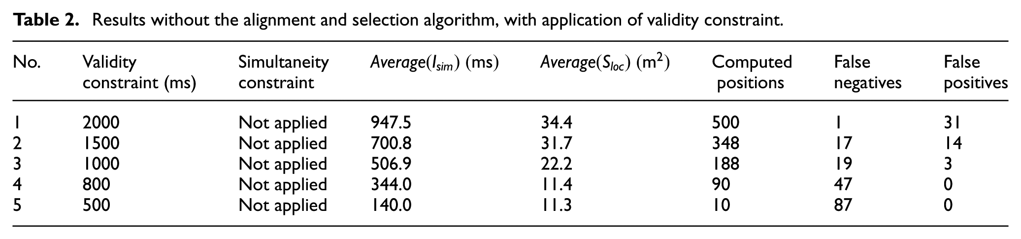
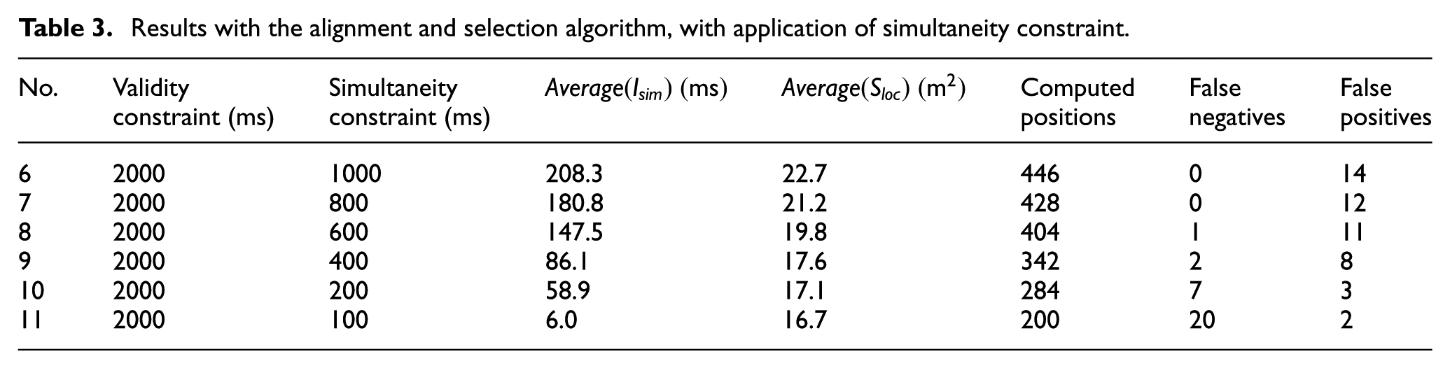
This section presents the results of a total of 11 experiments. The results for the first five experiments are presented in Table 2. During these experiments, the temporal alignment and selection algorithm and simultaneity constraint were not applied. The results of the application of temporal alignment and selection algorithm on stream elements and the use of different simultaneity constraints are presented in Table 3. In both tables, column no. 4 contains measured average simultaneity intervals for fusion inputs (a measure of temporal consistency of inputs) and column no. 5 contains average rectangular area of intersection points, which represents the precision of fusion result (a position of a passing vehicle). The results for $I_{sim}$ and $S_{loc}$ are averaged for each experiment, which is 30 min. The next column presents the number of completed fusions (successful fusion means that a position that satisfied spatial constraints was computed), and the last two columns show how many of the fusion results were false negatives and false positives. A false negative is a vehicle that was undetected and a false positive is a computed position where there were actually no vehicles present. We are able to find false positives and negatives because the time intervals when a vehicle was in range of the sensors were recorded during the original field experiment.

Table 2.

Results without the alignment and selection algorithm, with application of validity constraint.

No.	Validity constraint (ms)	Simultaneity constraint	$Average (I_{sim}) (ms)$	$Average (S_{loc}) (m^{2})$	Computed positions	False negatives	False positives
1	2000	Not applied	947.5	34.4	500	1	31
2	1500	Not applied	700.8	31.7	348	17	14
3	1000	Not applied	506.9	22.2	188	19	3
4	800	Not applied	344.0	11.4	90	47	0
5	500	Not applied	140.0	11.3	10	87	0

Table 3.

Results with the alignment and selection algorithm, with application of simultaneity constraint.

No.	Validityconstraint (ms)	Simultaneityconstraint (ms)	$Average (I_{sim}) (ms)$	$Average (S_{loc}) (m^{2})$	Computedpositions	False negatives	Falsepositives
6	2000	1000	208.3	22.7	446	0	14
7	2000	800	180.8	21.2	428	0	12
8	2000	600	147.5	19.8	404	1	11
9	2000	400	86.1	17.6	342	2	8
10	2000	200	58.9	17.1	284	7	3
11	2000	100	6.0	16.7	200	20	2

During the first five experiments presented in Table 2, the fusion node consumed the arrived inputs as freshest data first, in the same order as they arrived. A considerably long average simultaneity interval achieved can be explained by periodic and asynchronous execution of ad hoc WSN nodes. Furthermore, the allowable age for the freshest available sensor reading for transmission depends on the validity interval. With validity being longer than sensor process execution period, the sensor node was allowed to transmit or retransmit older values. The experiments 1–5 show that when the value of validity constraint is reduced, the values of $I_{sim}$ and $S_{loc}$ improve. However, the number of false negatives quickly rises. The lower values of validity interval filter out the sensor readings with longer delays. This does not improve the fusion reliability as with lower values of validity intervals more cars are left undetected. The effect can be explained by Figure 11, which presents a histogram from experiment 1 with measured sensor delays by fusion node A. During this experiment, the validity interval of sensor readings was 2000 ms, meaning the sensor is allowed to retransmit the valid readings if there are no newer readings. The figure is illustrative as it depicts the delays without the application of temporal constraints.

Figure 11.

Sensor delays measured on fusion node time axis.

The average for all delays of sensor readings received by the fusion node is 1357.7 ms. Altogether, the fusion node A received 9157 sensor readings. It can be observed that (due to periodic execution) the majority of the readings fall into an interval between 500 and 2000 ms. The reason why there is ca. 200 ms delay before the first readings arrive to the fusion node must be, in addition to the sensor sampling time, fusion node’s asynchronous and periodic execution. The readings that have been delayed more than 2000 ms are most likely the ones that were retransmitted due to no new valid readings. The theoretical maximum of a delay due to periodic execution and retransmission can be up to 3000 ms (validity time added to delay caused by periodic execution of processes). Longer delays must have been caused by network and environment induced uncertainties (or other real-world unpredictable causes).

The rest of the experiments (6–11) in Table 3 show how averaged values for simultaneity interval and area of location estimation are influenced by alignment and selection algorithm together with different values for simultaneity constraints.

The experiment indicates a correlation between simultaneity constraint and the area of average location estimation. The lower the simultaneity constraint, the smaller the area, that is, the precision of position estimation improves. However, the same side effect as during the first five experiments without the temporal alignment and selection algorithm is present. Stricter simultaneity constraint filters out the actual vehicle detections with lower precision (larger values of $S_{loc}$ ). For example, the usage of simultaneity constraint 100 ms leaves 20 vehicles undetected (false negatives).

Experimental results of the two different experiment configurations (freshest data first vs time-selective strategy) clearly show that time-selective approach achieves considerably better results than the configuration which uses only validity constraints and prefers the freshest data first.

Choosing a good criterion for WSN performance is not trivial. One possibility is to use accuracy as a criterion. In statistical tests, the accuracy can be measured by formula $Acc = (TP + TN) / (TP + FP + FN + TN)$ , where Acc = accuracy, TP = True Positives, TN = True Negatives, FP = False positives and FN = False Negatives. As we can see, the accuracy is increased if either false positives or false negatives or both are decreased. For these experiments, we consider a low number of false positives as the most important outcome. This number should be low as we do not want false alarms and if possible prefer to avoid the positions computed based on false alarms. Considering the results of all experiments carried out, the minimum acceptable number of false positives is chosen as three. The other outcome parameters to be considered are average area of computed positions $S_{loc}$ , the number of computed positions (successful fusions) and the number of false negatives.

With the first experiment configuration (the freshest data first approach), the best results are with validity constraint being 1000 ms, which is the first threshold, where the number of false positives is three. However, the number of false negatives is too high, 19 false negatives out of 92 vehicles leaves 20.7% of vehicles undetected. In total, this leaves only 73 vehicles detected with 185 correct positions. The average precision of positions was $22.2 m^{2}$ .

The second configuration shows much better results. The outcome of simultaneity constraint of 200 ms gives three false positives and less than 7.6% of false negatives. In total, 85 vehicles of 92 were detected with 281 correct positions. The average precision of positions was $17.1 m^{2}$ . It can be noticed that the average $S_{loc}$ is getting more stable after the simultaneity constraint of 400 ms. This indicates that more precise average position is difficult to achieve (the reason for this could be that the frame start is chosen as timestamp for sensor readings, not actual sound event).

In conclusion, with the same number of false positives in experiments 3 and 10, the second experiment configuration with time-selective algorithm showed significantly less false negatives (decreased by more than six times). Experiment 10 also improves the $Average (S_{loc})$ by 23.0%. When using more strict constraints in either configurations (with experiments 4, 5 or 11), the constraints start to filter out too many detections. We conclude also that the constraints were too relaxed in experiments 1, 2, 3, 6, 7, 8 and 9. The task of this article was not to find best configuration, but to give indication for the necessity of time-selective handling of input data for in-network processing.

Conclusion

Various situations exhibit physical phenomena which can be observed and measured with individual sensors practically simultaneously. The parallelism in the observation process is important, as it is otherwise difficult to combine these measurements during a fusion process later. We do not consider global clock synchronization feasible in an ad hoc WSNs, neither is the data transport time deterministic in such networks. The in-network data processing nodes receive packets out of order and with time varying delays, in addition sensor nodes themselves are unreliable. The purpose of this article was to show that using a time-selective strategy for in-network processing improves the temporal consistency of input data for SA information acquired in ad hoc WSN. To demonstrate the improvement, we used distributed autonomous sensors for detection of moving vehicles in an urban street. By applying the time-selective data fusion strategy, the fusion algorithm is able to select temporally compatible data from the arriving streams of sensor data. The data which satisfy simultaneity constraints have a higher probability for describing the observed situation accurately. After alignment and selection of temporally compatible data, the data still need to be checked against spatial constraints. As the data fusion considered in this article computes the position from distributed observations, the spatial check is done by the fusion process. Spatial constraints were briefly discussed in our earlier paper,⁴ and an idea of combining of temporal and spatial constraints has been discussed in Mõtus et al.³⁹ This area is a topic for a separate research paper.

We also consider the time-selective strategy generic enough to be applied in ad hoc WSNs regardless of media access control and link layer protocols. Furthermore, we consider that it is worth to research whether the time-selective data fusion strategy improves the effectiveness of filtering-based multi-sensor multi-lag OOSM approach for WSNs.

Footnotes

Handling Editor: Jose Molina

Declaration of conflicting interests

The author(s) declared no potential conflicts of interest with respect to the research, authorship, and/or publication of this article.

Funding

The author(s) disclosed receipt of the following financial support for the research, authorship, and/or publication of this article: This work was partially funded by the project SMENETE (Smart Environment Networking Technologies), which is funded by the European Regional Development Fund within the framework of EU Smart Specialisation programme 2014–2020 and the Estonian IT Academy program.

ORCID iD

Jaanus Kaugerand

References

Preden

Kaugerand

Suurjaak

et al . Data to decision: pushing situational information needs to the edge of the network. In: Proceedings of the 2015 IEEE international multi-disciplinary conference on cognitive methods in situation awareness and decision, Orlando, FL, 9–12 March 2015, pp.158–164. New York: IEEE.

Endsley

MR.

Designing for situation awareness: an approach to user-centered design. Boca Raton, FL: CRC Press, 2016.

Diallo

Rodrigues

Sene

Real-time data management on wireless sensor networks: a survey. J Netw Comput Appl 2012; 35(3): 1013–1021.

Ehala

Kaugerand

Pahtma

et al . Situation awareness via internet of things and in-network data processing. Int J Distrib Sens N 2017; 13(1): 686578.

Preden

Motus

Pahtma

et al . Data exchange for shared situation awareness. In: Proceedings of the 2012 IEEE international multi-disciplinary conference on cognitive methods in situation awareness and decision support (CogSIMA), New Orleans, LA, 6–8 March 2012, pp.198–201. New York: IEEE.

Yamaguchi

Watanabe

Sato

et al . In-vehicle distributed time-critical data stream management system for advanced driver assistance. J Inform Process 2017; 25: 107–120.

Cugola

Margara

. The complex event processing paradigm. In: Colace

De Santo

Moscato

et al . (eds.) Data management in pervasive systems. Cham: Springer, 2015, pp.113–133.

Abdelgawad

Bayoumi

Data fusion in WSN. In: Ahmed

Magdy

(eds) Resource-aware data fusion algorithms for wireless sensor networks. New York: Springer, 2012, pp.17–35.

Bartos

A survey of protocols for intermittently connected delay-tolerant wireless sensor networks. J Netw Comput Appl 2014; 41: 411–423.

10.

Mõtus

Rodd

MG.

Timing analysis of real-time software. New York: Elsevier, 1994.

11.

Izadi

Abawajy

Ghanavati

et al . A data fusion method in wireless sensor networks. Sensors 2015; 15(2): 2964–2979.

12.

Al-Anbagi

Erol-Kantarci

Mouftah

HT.

A survey on cross-layer quality-of-service approaches in WSNS for delay and reliability-aware applications. IEEE Commun Surv Tut 2016; 18(1): 525–552.

13.

Zhao

Wireless sensor networks for industrial process monitoring and control: a survey. Netw Protocol Algorithm 2011; 3(1): 46–63.

14.

Hiromori

Uchiyama

Yamaguchi

et al . Deadline aware data collection in CSMA/Ca-based multi-sink wireless sensor networks. In: Proceedings of the 6th international conference on mobile computing and ubiquitous networking (ICMU), vol. 12, Fukuoka, Japan, 23–24 May 2012, pp.284–294. Tokyo: IPSJ.

15.

Cheng

Leung

Maupin

A delay-aware network structure for wireless sensor networks with in-network data fusion. IEEE Sens J 2013; 13(5): 1622–1631.

16.

Wang

Vuran

Goddard

Cross-layer analysis of the end-to-end delay distribution in wireless sensor networks. IEEE/ACM T Network 2012; 20(1): 305–318.

17.

Oliver

Fohler

. Probabilistic estimation of end-to-end path latency in wireless sensor networks. In: Proceedings of the IEEE 6th international conference on mobile Ad hoc and sensor systems (MASS’09), Macau, China, 12–15 October 2009, pp.423–431. New York: IEEE.

18.

Preden

Llinas

Rogova

et al . On-line data validation in distributed data fusion. In: Proceedings of the international conference on SPIE defense, security, and sensing, vol. 8742. Baltimore, MD, 22 May 2013. Bellingham, WA: SPIE.

19.

Kopetz

Real-time systems: design principles for distributed embedded applications. New York: Springer, 2011.

20.

Maroti

Sallai

Packet-level time synchronization. Technical report, TinyOS Core Working Group, Berkeley, CA, 2008.

21.

Carrano

Passos

Magalhaes

et al . Survey and taxonomy of duty cycling mechanisms in wireless sensor networks. IEEE Commun Surv Tut 2014; 16(1): 181–194.

22.

Khaleghi

Khamis

Karray

et al . Multisensor data fusion: a review of the state-of-the-art. Inform Fusion 2013; 14(1): 28–44.

23.

Liu

Wang

Liu

et al . Data-aware retrodiction for asynchronous harmonic measurement in a cyber-physical energy system. Sensors 2016; 16(8): 1316.

24.

Sun

Lin

et al . Multi-sensor distributed fusion estimation with applications in networked systems: a review paper. Inform Fusion 2017; 38: 122–134.

25.

Shi

Wan

A unified out-of-sequence measurements fusion algorithm for WSN. In Proceedings of the 1st international workshop on database technology and applications, Wuhan, China, 25–26 April 2009, pp.76–79. New York: IEEE.

26.

Xiaoliang

Chenglin

Lizhong

Multi-sensor multi-OOSM distributed sequential fusion filtering. In: Proceedings of the 10th IEEE international conference on control and automation (ICCA), Hangzhou, China, 12–14 June 2013, pp.77–776. New York: IEEE.

27.

Yadav

Chitra

Deepika

CL.

Reviewing the process of data fusion in wireless sensor network: a brief survey. Int J Wireless Mob Comput 2015; 8(2): 130–140.

28.

Bahrepour

Meratnia

Havinga

PJM

. Sensor fusion-based event detection in wireless sensor networks. In: Proceedings of the 6th annual international mobile and ubiquitous systems: networking services (MobiQuitous), Toronto, ON, Canada, 13–16 July 2009, pp.1–8. New York: IEEE.

29.

Lai

Cao

Fan

. Ted: efficient type-based composite event detection for wireless sensor network. In: Proceedings of the 11th international conference on distributed computing in sensor systems (DCOSS), Barcelona, 27–29 June 2011, pp.1–8. New York: IEEE.

30.

Jacoub

Liscano

Bradbury

. A survey of modeling techniques for wireless sensor networks. In: Proceedings of the 5th international conference on sensor technologies and applications (SENSORCOMM), vol. 2011, Nice, 21–27 August 2011, pp.103–109. IARA XPS Press.

31.

Jhumka

Bradbury

Saginbekov

Efficient fault-tolerant collision-free data aggregation scheduling for wireless sensor networks. J Parallel Distr Com 2014; 74(1): 1789–1801.

32.

Dearle

Balasubramaniam

Lewis

et al . A component-based model and language for wireless sensor network applications. In: Proceedings of the 32nd annual IEEE international conference on computer software and applications (COMPSAC’08), Turku, 28–1 August 2008. pp.1303–1308. New York: IEEE.

33.

Eidson

Lee

Matic

et al . Distributed real-time software for cyber–physical systems. Proc IEEE 2012; 100(1): 45–59.

34.

Mõtus

Meriste

Preden

JS.

Towards middleware based situation awareness. In: Proceedings of the IEEE military communications conference (MILCOM), Boston, MA, 18–21 October 2009, pp.1–7. New York: IEEE.

35.

Preden

Llinas

Motus

. Middleware for exchange and validation of context data and information. In: Snidaro

García

Llinas

et al . (eds) Context-enhanced information fusion. New York: Springer, 2016, pp.205–230.

36.

Sarvghadi

Wan

TC.

Message passing based time synchronization in wireless sensor networks: a survey. Int J Distrib Sens N 2016; 12(5): 1280904.

37.

Djenouri

Bagaa

Synchronization protocols and implementation issues in wireless sensor networks: a review. IEEE Syst J 2016; 10(2): 617–627.

38.

Cruz

JRP

Hernandez

SEP

. Temporal alignment model for data streams in wireless sensor networks based on causal dependencies. Int J Distrib Sens N 2014; 10(3): 938698.

39.

Mõtus

Preden

Meriste

et al . Self-aware architecture to support partial control of emergent behavior. In: Proceedings of the 7th international conference on system of systems engineering (SoSE), Genova, 16–19 July 2012, pp.422–427. New York: IEEE.

Time-selective data fusion for in-network processing in ad hoc wireless sensor networks

Abstract

Keywords

Introduction

Related work

Modelling data streams and time-selective data fusion in WSN

Sensor readings arriving out of order

Modelling time-selective data fusion in WSN

Temporal validity interval of input data

Fusion requires overlapping validity of stream elements

Simultaneity interval

Alignment and selection of compatible elementsfrom streams

Accumulated delays of the sensor readings

Experiment setup

Location estimation by fusion nodes

Experiment configurations

Results

Conclusion

Footnotes

Declaration of conflicting interests

Funding

ORCID iD

References