
Abstract
In this article we propose several new progress based, localized, power, and cost aware algorithms for routing in ad hoc wireless networks. These algorithms attempt to minimize the total power and/or cost needed to route a message from source to destination. In localized algorithms, each node makes routing decisions solely on the basis of location of itself, its neighbors and destination. The new algorithms are based on the notion of proportional progress. A node currently holding the packet will forward it to a neighbor, closer to destination than itself, which minimizes the ratio of power and/or cost to reach that neighbor, and the progress made, measured as the reduction in distance to destination, or projection along the line to destination. First, we propose Power Progress, Iterative Power Progress, Projection Power Progress, and Iterative Projection Power Progress algorithms, where the proportional progress is defined in terms of power measure. The power metrics are then replaced by cost or power-cost metrics to define the proportional progress in terms of cost or power-cost measure, resulting in the cost and power-cost variants of the above algorithms. All the new proposed methods are implemented and their performances are compared with other competitive localized algorithms, shortest path. NC (Nearest Closer), and greedy schemes. The new power and cost localized schemes are conceptually simpler than existing schemes, and have similar or somewhat better performance in our experiments. Our localized schemes are shown to be competitive with globalized shortest weighted path based schemes.
Introduction
Due to its potential applications in various situations such as a battlefield, emergency relief, environment monitoring, etc., wireless ad hoc networks [1, 2] have recently emerged as a premier research topic. Such networks consist of hosts that communicate without a fixed infrastructure. Communications take place over a wireless channel, where each host has the ability to communicate with others in the neighborhood, determined by the transmission range. Since there is no infrastructure, every host has to determine its environment when the network is formed.
We assume that each node has a low-power Global Position System (GPS) receiver, which provides the position information of the node itself. If GPS is not available, the distance between neighboring nodes can be estimated on the basis of incoming signal strengths. Relative co-ordinates of neighboring nodes can be obtained by exchanging such information between neighbors [3]. We assume nodes with identical capabilities.
In the routing task, a message is to be sent from a source node to a destination node. Due to propagation path loss, the transmission radii are limited and routes between two hosts in the network may consist of hops through other hosts in the network. The nodes in the network may be static or mobile. The task of finding and maintaining routes in ad hoc networks is nontrivial since host mobility can result in unpredictable topology changes. We assume in this article that the source node is aware of the geographic position of destination. Location updates schemes for efficient routing are reviewed in [4]. Many routing algorithms proposed are non-local and require the complete knowledge and maintenance of the network topology. Recently, many localized routing algorithms have been proposed (a brief survey of them is given in [5]), where nodes do not require the complete network topological information to perform the routing task. More precisely, nodes only require the position of itself and its 1-hop neighbors, and position of destination. Consequently, neighboring nodes are aware of distances between them.
Desirable qualitative properties of routing protocols include: distributed operation, loop freedom, demand-based operation, and ‘sleep’ period operation while hop count and delivery rates are among quantitative metrics. Because of the limited battery power at each node, the developers of routing protocols should have the following goals in mind:
Minimize energy required per routing task: Hop count was traditionally used to measure energy requirements of a routing task, thus using constant metric per hop. However, if nodes can adjust their transmission power, with the knowledge of their neighbor locations, the constant metric can be replaced by a power metric that depends on the distance between nodes [9, 11]. As discussed earlier, the distance between nodes can be estimated on the basis of incoming signal strengths or by using Global Positioning System, if nodes are equipped with a small GPS receiver. Maximize the number of routing tasks that the network can perform: Some nodes participate in routing packets for many source destination pairs and the increased energy consumption may result in their failure. Thus, pure power consumption metric may be misguided in the long term [10]. A longer path that passes through nodes that have plenty of energy may be a better solution [10]. Alternatively, some nodes in the sensor or ad hoc network may be temporarily inactive and power consumption metric may be applied on active nodes. Minimize communication overhead: Due to limited battery power, the communication overhead must be minimized if the number of routing tasks is to be maximized. Node mobility and changes in activity status (between active and sleep periods) make proactive methods prohibitively expensive, as the maintenance overhead defeats the claimed energy savings. Methods that maintain routing tables with up-to-date routing information or global network information at each node are certainly unsatisfactory solutions. This goal is achieved by using localized algorithms. Localized algorithms are distributed algorithms that resemble greedy methods, where simple local behavior achieves a desired global objective. In a localized routing algorithm, each node makes a decision to forward the message to a neighbor, solely based on the locations of itself, it's neighbors and the destination. All non-localized routing techniques proposed in the literature are variations of shortest weighted path algorithm [10, 9].
Stojmenovic and Lin [8] described the first localized power and cost aware routing protocols for ad hoc networks. In this article, we revisit the problem and propose several such new protocols. In our new schemes, a node currently holding the packet will forward it to a neighbor, closer to destination than itself, which minimizes the ratio of power and/or cost to reach that neighbor, and the progress made, measured as the reduction in distance to destination, or projection along the line to destination. In power progress algorithm, a node S currently holding the packet, will forward it to a neighbor A, that minimizes (|SA| α + c)/(|SD| − |AD|), where α is the power attenuation factor between 2 and 6. c is the constant and D is the destination. In iterative power progress algorithm, we first find a node A that minimizes power (|SA|)/(|SD| − |AD|) as in power progress scheme, and then iteratively find an intermediate node B (B is closer to D than S) with minimum (power(|SB|) + power(|BA|)) measure, while satisfying power(|SB|) + power(|BA|) < power(|SA|). In projection power progress algorithm, a neighbor node that minimizes (|SA|α + c)/(SD · SA) is chosen to forward the message, where (SD · SA) is the dot product of two vectors. The iterative projection power progress algorithm is very similar to the iterative power progress algorithm, except that the first forwarding node is found using the projection power progress technique. Power metrics in the above algorithms can be replaced by a cost or power-cost metrics to define the proportional progress in terms of cost or power-cost measure, resulting in cost and power-cost variants of the above algorithms.
We compare the performances of power and cost/power-cost algorithms separately. For the power algorithms, the performance metrics used to compare the various algorithms are the total amount of power required to successfully route a message from the source to the destination and the success rates in finding a route successfully from the source to the destination. For the cost/power-cost algorithms, the performance metric used to compare the algorithms is the number of routing tasks that can be successfully performed before the power of any one of the nodes in the network reaches zero. We compare the performance of the new algorithms with the localized techniques described in [8] and shortest path, NC (Nearest Closer) and greedy schemes.
The rest of the article is organized as follows. In Section 2, we present related work in this area. Section 3 presents the Power Progress, Cost Progress, Power-cost Progress algorithms and their iterative variants. Projection Power Progress, Projection Cost Progress, Projection Power-cost Progress algorithms and their iterative versions are also presented. Results of our simulation and performance study are presented in Section 4. In Section 5, we provide concluding remarks and list some open problems in this area.
The preliminary conference version of this article is published as [13].
Related Work
In most routing protocols, the paths are computed based on minimizing hop count or delay. When transmission power of nodes is adjustable, hop count may be replaced by power consumption metrics. Some nodes participate in routing packets for many source-destination pairs, and the increased energy consumption may result in their failure. A longer path that passes through nodes that have plenty of energy may be a better solution [10]. The goals of the routing protocol design, are therefore to minimize the energy per routing taks, and to maximize the number of routing tasks the network can perform. A survey of power optimization techniques for routing protocols in wireless networks can be found in [12]. Also, there exist a vast amount of literature devoted to localized routing in ad hoc networks.
Existing Power Aware Routing Algorithms
Rodoplu and Meng [9] proposed a general model in which the power consumption between two nodes at distance d is u(d) = dα + c for some constants α (2 < α < 5) and c. They described several properties of power transmission that can be used to find neighbors for which direct transmission is the best choice in terms of power consumption, and proposed a non-localized proactive power aware routing scheme. Constant factor c in this expression for total energy consumption includes the energy consumed in computer processing and encoding/decoding at both transmitter and receiver nodes and minimal reception power even when nodes are at zero distance: therefore c > 0. In their experiments, they adopted the model with u(d) = d4 + 2*108, which we refer as the RM Model. They described a routing algorithm that runs in two phases. In the first phase, each node searches for its neighbors and selects these neighbors for which direct transmission requires less power than if an intermediate node is used to retransmit the message. In the second phase, each possible destination runs a distributed loop free variant of the non-localized Bellman-Ford algorithm and computes shortest path for each source. The same algorithm is run from each possible destination.
Heinzelman et al. [11] used signal attenuation to design an energy efficient routing protocol for wireless micro-sensor networks, where destination is fixed and known to all nodes. They propose to utilize a 2-level hierarchy of forwarding nodes, where sensors form clusters and elect a random cluster-head. The cluster-head forwards transmission from each sensor within its own cluster. This scheme is shown to save energy under some conditions. We refer to their model as the HCB Model, where power needed for transmission and reception at distance d is u(d) = d2 + 2*1000.
If nodes have information about position and activity of all other nodes in the network, then the optimal power saving algorithm, that minimizes the total energy per packet, can be obtained by applying Dijkstra's single source shortest weighted path algorithm. Each edge weight is then set as u(d) = adα + c, where d is the length of the edge. We refer to it as SP Power algorithm, which is used to compare the performance of our new localized algorithms.
Localized power aware algorithms have been proposed earlier by Stojmenovic and Lin [8]. They show how to convert a polynomial function in d (with exponent α) for power consumption (in case of direct transmission from sender to destination) to a linear function in d by retransmitting the packet via some intermediate nodes that might be available, where d = |SD| is the distance between the source S and the destination D. The power needed for direct transmission is u(d) = adα + c which is optimal if d < (c/(a(1 − 2I α)))(1/α). Otherwise, n − 1 equally spaced nodes can be selected for retransmissions, where n = d(a(α − 1)/c)(1/α) (rounded to the nearest integer), producing minimal power consumption of about v(d) = dc(a(α − 1)/c)(1/α) + da(a(α − 1)/c)(1-α)/α. In reality there are no nodes at the desired locations; nevertheless it gives a good idea of how far one hop should approximately advance for minimizing energy per routing task. In their [8] power efficient, localized algorithm, a source node S holding the message selects a neighbor node A (which is closer to destination than S) to forward the message, which minimizes p(S.A) = u(r) + v(s), where r = |AS| and s = |AD|. For α = 2 it becomes u(r) + v(s) = ar2 + c + 2s(ac)1/2. If destination D is a neighbor of S then compare the expression with the corresponding one, u(d) = adα + c, needed for direct transmission (s = 0 for D, and D can be treated as any other neighbor). The algorithm proceeds until the destination is reached, if possible. In Section 4 of this article, we refer to this algorithm as the Power algorithm.
The authors in [8] also proposed the NC algorithm, where node, currently holding the message, will forward it to the nearest neighbor. Only nodes closer to destination than the current node are considered.
Finn [6] proposed a localized greedy scheme, where a node, currently holding the message, will forward it to the neighbor that is closest to destination. Only nodes closer to destination than the current node are considered.
Existing Cost and Power-cost Routing Algorithms
Singh et al. [10] proposed to use a function f(A) to denote node A's reluctance to forward packets, and to choose a path that minimizes the sum of f(A) for nodes on the path. This routing protocol [10] addresses the issue of energy critical nodes. As a particular choice for f, [10] proposes f(A) − 1/g(A) where g(A) denotes the remaining lifetime (g(A) is normalized to be in the interval [0,1]). Thus reluctance grows significantly when lifetime approaches 0. The reluctance f(A) is used as a weight in a shortest weighted path algorithm. In our experiments, we refer to this optimal algorithm as the SP Cost algorithm while comparing the performances of the newly proposed cost algorithms in Section 4. The other metric used in [10] is aimed at minimizing the total energy consumed per packet. However the article merely observes that the routes selected when using this metric would be identical to the shortest hop count routing since the energy consumed in transmitting and receiving one packet over one hop is considered a constant.
A cost aware localized algorithm, assuming constant power for each transmission, was proposed in [8]. The cost c(A) of a route from B to D via neighboring node A is the sum of the cost f(A) = 1/g(A) of node A and the estimated cost of route from A to D. The cost f(A) of each neighbor A of node S currently holding the packet is known to B. In [8], the cost of remaining path is assumed to be proportional to the number of hops between A and D. The number of hops, in turn, is proportional to the distance d − |AD|, and inversely proportional to radius R. Thus the cost is td/R, where factor t is to be investigated separately. The cost c(A) of a route from S to D via A is then estimated to be c(A) = f(A) + td/R. If destination is one of the neighbors of node B currently holding the packet then the packet will be delivered to D. Otherwise, S will select one of its neighbors A which will minimize c(A). The algorithm proceeds until the destination is reached, if possible, or a node has no closer node to destination than itself. The algorithm Cost-ii [8], where t = f(A) is used to compare the performance of our new cost based algorithms.
Stojmenovic and Lin [8] also proposed two different ways to combine power and cost metrics into a single power-cost metric, based on the product and sum of two metrics, respectively. If the product is used, then the power-cost of sending message from S to a neighbor A is equal to powercost(S, A) = f(A)u(r) (where |AS| = r). The sum, on the other hand, leads to a new metrics powercost(S, A) = au(r) + bf(A), for suitably selected values of a and b. The authors defined a power-cost efficient routing algorithm [8] as follows. The node S currently holding the message will forward it to a neighbor A that minimizes pc(S, A) − powercost(S, A) (u(r) + p(d)). We use the powercost product version and refer to it as the PowerCost2 algorithm in our comparison study. This choice avoids using parameters and is competitive with other options [8].
The optimal power-cost route can be computed by applying Dijkstra's shortest path algorithm where the node's powercost value is transferred to the edge leading to the node. In Section 4, we refer to this optimal algorithm as the SP Power*Cost algorithm for our comparisons.
New Power and Cost Aware Algorithms
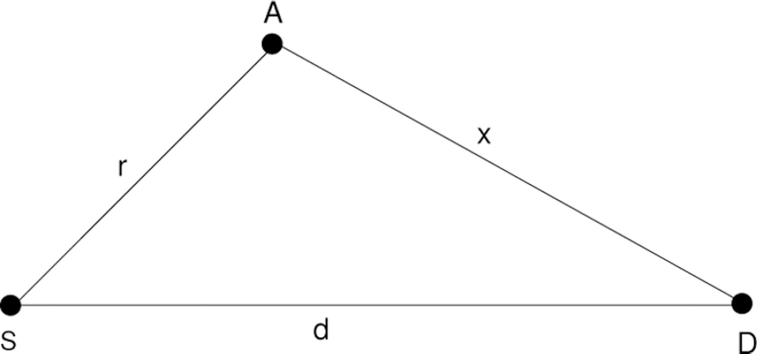
Let the current node holding the packet be S, destination be D, and A be a neighbor of S as in Fig. 1. Let |SA| = r, |SD| = d, and |AD| = x, with x < d. The new Power Progress algorithm is based on the notion of proportional progress. Let us measure the proportional progress as the power used to make a portion of the progress. The power needed to send from S to A is rα + c. The portion of progress made with it is (d − x). With similar advance continuing, there would be d/(d − x) such steps, and the total cost would be (rα + c)d/(d − x). Therefore the neighbor A that would minimize (rα + c)/(d − x) will be selected for forwarding the message. This means that the selected neighbor minimizes the power spent per unit of progress made, in terms of getting closer to the destination. Power metrics can be similarly replaced by a cost or power-cost metric to define cost or power-cost per unit of progress made. This leads to the Cost Progress and Power-Cost Progress algorithms that select forwarding neighbors that minimize f(A)/(d − x), and f(A)(rα + c)/(d − x), respectively.
Selecting the best neighbor in localized routing protocols.
The Projection Power Progress, Projection Cost Progress, and Projection Power-Cost Progress algorithms differ from the power progress algorithms in terms of the measure of proportional progress made. In projection progress based algorithms, node S currently holding the message will forward to a neighbor A that minimizes (rα + c)/(SD·SA), where (SD · SA) is the dot product of two vectors.
The Iterative Power Progress algorithm is an improvement of the Power Progress algorithm. It can be described as follows. As in Power Progress, a node S currently holding message will first find a neighbor A that minimizes (rα + c)/(d − x). Then, an intermediate node B (closer to destination than S, if exists) is found (that is neighbor to both S and A) which satisfies (power(|SB|) + power(|BA|)) < power(|SA|) and has the minimum (power(|SB|) + power(|BA|)) measure. If found, such node B replaces A as selected neighbor, and the search for even better intermediate node B repeats. This process is iteratively repeated until no improvement is possible and node S will forward the message to the selected neighbor (see Fig. 2). Which then applies again the same scheme for its own forwarding.

Selecting the best neighbor in the iterative versions.
A pseudo code of the algorithm can be written as follows.

Iterative Power-Cost Progress algorithm can be similarly defined. There is no iterative version defined for the Cost Progress algorithm, since the overall cost increases by adding intermediate nodes on a path.
The Iterative Projection Progress scheme is very similar to the Iterative Power Progress scheme, except that the first candidate node A is found using the projection progress method, (minimizes (rα + c)/(SD · SA)), instead of power progress scheme. Iterative Projection Power Progress and Iterative Projection Power-Cost Progress are the iterative versions of Projection Power Progress and Projection Power-Cost Progress algorithms.
Evaluation of Power Aware Algorithms
In this section, we present the results of our simulation study of the different power algorithms. First, we studied the effect of different squares (placement areas) on various algorithms. We used squares of size 50, 300, 500, 5000, and 50000 (for the HCB Model, α = 2, c = 2000). However, for the RM Model (α = 4, c = 2 * 108), we used square sizes 500, 1000, 5000, 10000, and 50000 to derive various relative performances with respect to selected α and c. Randomly generated connected graphs of density d = 20 were used with number of nodes fixed at n = 250. The network density d is defined as the average number of neighbors per each node. Dijkstra's shortest path scheme was used to test network connectivity, and only connected graphs were used in measurements. We used dense graphs because the success rate of all the algorithms then remained close to 100%, therefore the success rate was not a variable in these measurements.
The performance metric we have used to compare the performance of various algorithms is the total amount of power required to successfully route a message from the source to the destination (averaged over 500 randomly selected connected unit graphs and source destination pairs in each graph). We define power dilation as the ratio of the power requirement of the specific algorithm to that of SP Power, which is the optimal performing algorithm. We simulated, and compared the performance of power progress, iterative power progress, projection power progress, and iterative projection power progress with that of the power and NC algorithms from [8], greedy scheme [6] and global shortest path algorithms (with and without power weights).
Figure 3 and 4 present power dilations for various algorithms, with different square sizes, for the HCB Model and RM Model respectively. For α = 2, c = 0 and α = 4, c = 0 values, the power dilations remained stable for all square sizes. Figure 5 shows the average power dilations for α = 2 and α = 4, c = 0.

Power dilations for α = 2, c = 2000.

Power dilations for α = 4, c = 2 * 108.

Power dilations for α = 2 and α = 4, c = 0.
We can observe that the performance of the newly proposed localized routing algorithms are better than the performance of existing power aware scheme [8] for α = 2, c = 2000, and comparable for α = 4, c = 2 * 108. The iterative power progress method performed somewhat better for α = 4, c = 2 * 108 than power scheme [8]. Overall, all proposed schemes have very encouraging performance with respect to the optimal global SP Power algorithm, which is a significant achievement. The newly proposed methods reduced the excess power from 28% to 13% for the largest square size considered for α = 2, c = 2000. The excess power for α = 4, c = 2 * 108 is reduced to 69% for the largest square size considered. In all cases, the excess power rate has apparently slow increase with further square size increase. Similar comparison is obtained for c = 0. Our algorithms outperform the greedy and SP methods in all cases. For c > 0, the NC method is very inefficient at low square values, but comparable with other localized algorithms at high square values. For c = 0, the Power [8] and NC methods are identical.
NC performs poorly for small square sizes since the constant charge c is applied too frequently, making power consumption unnecessarily huge. For SP and Greedy algorithms, the performance drops drastically after some threshold square size due to the selection of longer hops, requiring significantly higher energy because of the power attenuation factor. The power dilation factor remains reasonably close after this threshold since the constant c then appears largely ignored, thus the choice of neighbors is not affected by further size increase. For square sizes before this threshold, the power dilation values are mostly influenced by the constant charge c.
As indicated in Figs. 3, 4, and 5, we can also classify the performances of these algorithms into different groups. With constant c > 0, the group of Power, Power Progress, and Iterative Power Progress algorithms have very similar power dilation results. Similarly, Projection Progress, and Iterative Projection Progress algorithms can be grouped together. However, with c = 0, based on similar performances, these algorithms can be grouped as indicated in Fig. 5. The Power and NC algorithms behave identical with c = 0.
We also compared the performance of considered algorithms with respect to their success rates for different densities, d = 6,8,10,20, and otherwise the same choices of parameters. The success rates of the various algorithms in finding a route successfully from the source to the destination for the HCB model (α = 2, c = 2000) is given in Fig. 6. Other α and c combinations produced very similar results. and thus we omitted the corresponding tables. We can observe that the success rates of newly proposed methods are similar to the success rates of the previously known power scheme [8].
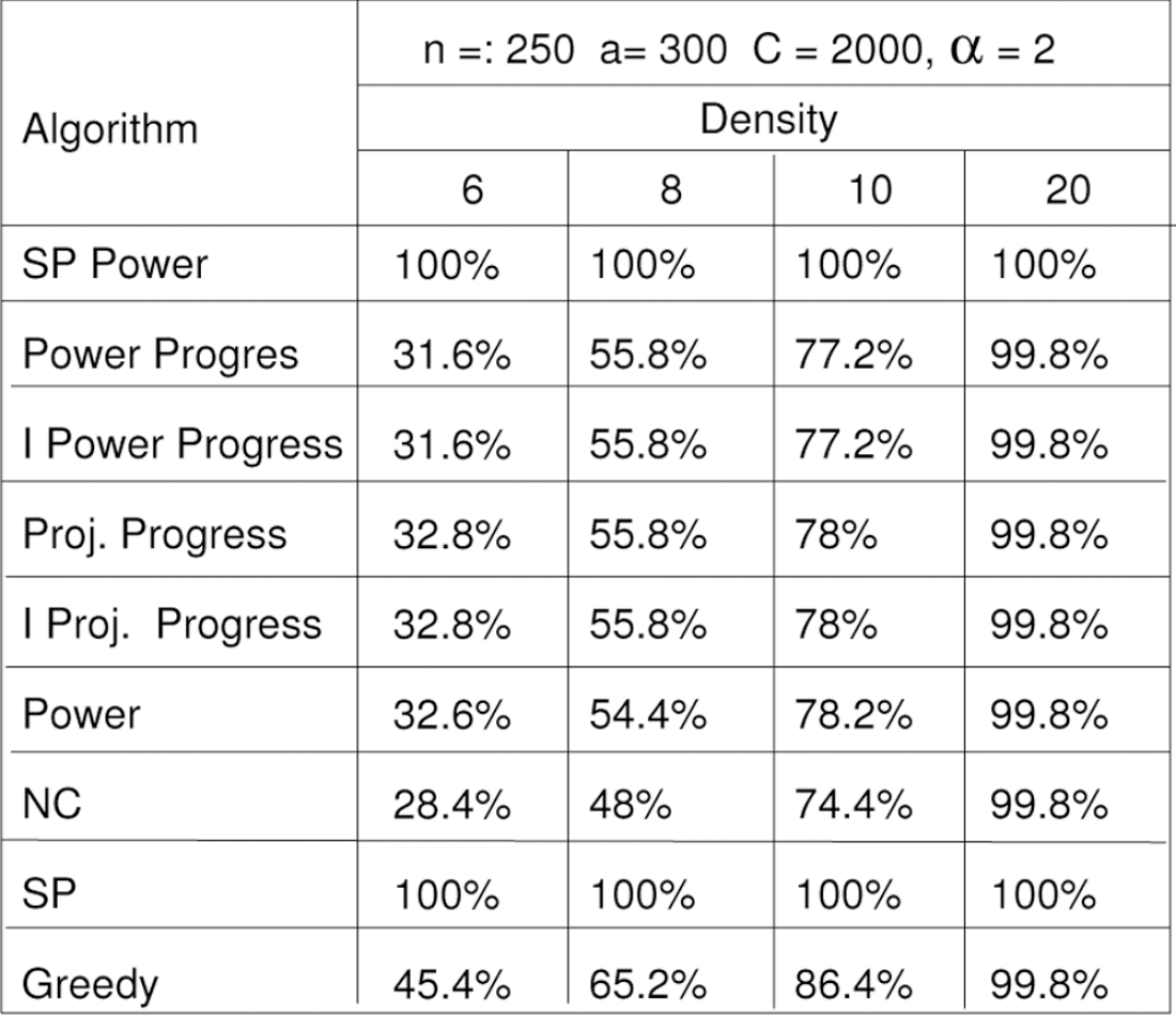
Success Rates for the HCB Model (α = 2, c = 2000).
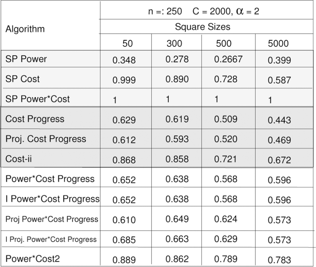
In this section, we present the results of our simulation and performance comparison of cost and power-cost algorithms. The performance metric used to compare the algorithms is the number of routing tasks that can be successfully performed before the power of any one of the nodes in the network reaches zero. We used squares of size 50, 300, 500, and 5000 (for the HCB Model, α = 2, c = 2000). However, for the RM Model (α = 4, c = 2 * 108), we used square sizes 500, 1000, 5000, 10000 and 50000 to derive various relative performances with respect to selected α and c. We generated high density connected graphs with 250 nodes placed in the chosen square size. Each node is assigned with an initial energy value, constant to all nodes in the network. A random source destination pair is selected and the route is calculated from the source to the destination using each algorithm. Once the path is computed, actual power required is charged to the nodes that are part of the calculated path. This process is repeated for the same graph, until a node has insufficient power to perform assigned task. The reported results are averaged over 10 graphs.
The initial power assignments to the nodes were 50K, 150K, 200K, and 5M for square sizes 50, 300, 500, and 5000 respectively, where K = 1000 and M = 1000000 for the HCB Model. For the RM Model, the initial power assignments were 8 * 108, 16 * 108, 9.5 * 1011, 13 * 1012, and 8 * 1015 for square sizes 500, 1000, 5000, 10000, and 50000 respectively. We compared the performances of global algorithms SP-Power, SP-Cost, SP-Power*Cost, newly proposed local algorithms Cost Progress, Power-Cost Progress, Iterative Power-Cost Progress, Projection Cost Progress, Projection Power-Cost Progress, Iterative Projection Power-Cost Progress and Cost-ii [8] PowerCost2 [8]. We define the iteration dilation as the ratio of the number of iterations of the algorithm to that of SP Power*Cost. Figures 7 and 8 show the results (expressed as iteration dilation ratios) for the HCB Model and the RM Model respectiveley. For c = 0, the iteration dilation ratios remained relatively same for different square sizes. Figure 9 shows the average iteration dilation ratios for the different square sizes. The newly proposed cost and power-cost aware localized algorithms are competitive with several already proposed in [8].
Iteration dilation ratios - HCB Model.

Iteration dilation ratios - RM Model.

Iteration Dilation Ratios for (α = 2, c = 0 and α = 4, c = 0).
This paper described several localized routing algorithms that attempt to minimize the total energy per routing task and maximize life time of each node. The localized nature of the protocols avoids the energy expenditure and communication overhead needed to build and maintain the global topological information. Our simulation results show that the performance of our localized algorithms is close to the performance of the shortest path algorithms, which require global knowledge.
It appears that we have achieved an optimal design for power aware localized algorithms. However, our experiments do not give an ultimate answer on the selection of approach that would give the most prolonged life to each node in the network. There is a need to consider further localized cost and power-cost aware routing schemes. In our future work, we also plan to address power and cost aware localized routing with a realistic physical layer.