Sage Journals: Discover world-class research

Abstract

Failure prediction for hard disk drives is a typical and effective approach to improve the reliability of storage systems. In a large-scale data center environment, the various brands and models of drives serve diverse applications with different input/output workload patterns, and non-ignorable differences exist in each type of drive failures, which make this mechanism much challenging. Although many efforts are devoted to this mechanism, the accuracy still needs to be improved. In this article, we propose a failure prediction method for hard disk drives based on a part-voting random forest, which differentiates prediction of failures in a coarse-grained manner. We conduct groups of validation experiments on two real-world datasets, which contain the SMART data of 64,193 drives. The experimental results show that our proposed method can achieve a better prediction accuracy than state-of-the-art methods.

Keywords

Failure prediction random forest clustering algorithm hard disk drives

Introduction

Large-scale storage systems are widely used in many sites, including high-performance computing systems and Internet service providers.¹ The unprecedented scales of storage systems greatly increase the incidence of hard disk drive (HDD) failure. The disastrous consequences of HDD failures can be permanent and difficult to be recovered, even unrecoverable, which leads to longer server down time and lower reliability of Internet data centers (IDCs).^2–4 To ensure the reliability and stability of systems, IDCs monitor the working conditions of HDDs in real time to detect soon-to-fail HDDs by sensors,^5–7 including accelerometers and acoustic emission sensors, thermal sensors, and counters. However, accuracy of these approaches is not promising.

SMART (self-monitoring and repair technology)^8,9 has been used to evaluate the health status of drives on the inner condition and environments data of HDDs provided by sensors and counters.¹⁰ Once it detects that an HDD will fail soon, it informs the system administrator, who should address this issue. Unfortunately, its failure detection rates (FDRs) are only 3%–10%.¹¹ Several methods have been proposed in the past decades to improve the accuracy of HDD failure prediction. Most algorithms apply statistical approaches, machine learning, and deep learning technologies, including rank-sum test,¹² naive Bayesian classifiers,⁵ support vector machine (SVM),^13,14 back-propagation neural networks (BPNNs),¹³ classification tree (CT),¹⁵ and recurrent neural networks (RNNs).¹⁶

These existing methods have achieved good prediction performance; however, three disadvantages remain. First, these methods use uniform classification rules to distinguish between the soon-to-fail and good drives. However, there are several types of drive failures, and the characteristics, degradation process, and correlated SMART attributes of them are all different^17,18 due to the complex electro-mechanical structures and mechanisms of HDDs. The result of this issue is that these methods are good at identifying frequent failures but perform poorly for failures that occur less often, which becomes a performance bottleneck of failure prediction. Second, the performance of these methods depends strongly on parameter optimization; however, various brands and modes of HDDs serve diverse applications with different input/output workload patterns in a data center environment, and as these context varies, parameters of a prediction model need to be tuned, which is a cumbersome task. Third, there is a huge difference in the number of failed and good drives in the real world. This data imbalance hinders the performance of HDD failure prediction.

Our goal is to develop an effective failure prediction method for HDDs by identifying soon-to-fail drives using differential classification rules. We propose a random-forest-based prediction method, which differentiates prediction of HDD failures in a coarse-grained manner. Random forest is an ensemble machine learning model for classification that operates by constructing a multitude of decision trees. This model utilizes the randomization of training samples and features to achieve good classification results, which greatly simplifies parameter optimization. The decision trees in the forest are not pruned, and each tree specializes in classifying a part of health samples rather than all of them.¹⁹ Considering the different correlated SMART attributes of various types of HDD failures, we take advantage of different combinations of decision trees to vote on the classification results so that their specialization can be leveraged. The part-voting strategy ensures the prediction model is more comprehensive to distinguish good drives and soon-to-fail drives.

To address the problem of data imbalance, we use under-sampling to further improve the prediction accuracy. However, under-sampling will lose the characteristic details of good samples, which leads to a high false alarm rate (FAR). To ensure that limited good samples in the training set can cover the characteristics as comprehensive as possible, we develop a clustering method to assist in the sampling, which increases the FDR without decreasing the FAR. Moreover, clustering-based under-sampling method can reduce the computation overhead and improve the efficiency of model training.

The main contributions of this article are as follows:

The proposed method based on part-voting random forest is capable of differentiating failure prediction for HDDs.

A clustering-based under-sampling method is presented, which addresses the data imbalance problem and improves the quality of training set.

We performed a comprehensive evaluation using the datasets from production data centers. The experimental results show that the prediction model can archive an FDR of over 97.67% with an FAR of 0.017% .

The remainder of this article is organized as follows. Section “Background and related work” reviews the background and related work, including HDD failures, SMART, and HDD failure prediction. Section “Prediction method based on part-voting random forest” describes the proposed prediction model and relevant algorithms. Section “Evaluation metrics” discusses the evaluation metrics for failure prediction. Section “Experimental results” gives the experimental results and a comparison with state-of-the-art failure prediction approaches. Section “Conclusion and future work” concludes the article.

Background and related work

HDD failure

There exist non-ignorable differences in the characteristics and deterioration processes of different types of HDD failures.¹⁷ The diversity of HDD failures is the result of the complex structure and mechanism of HDDs. A HDD is composed of four units: the head disk interface, the head stack assembly, spindle motors/bearing, and the electronics module.¹⁸ Because the mechanisms of these units are quite different, the trigger factors of their failures are distinct from each other. For example, the head–disk interface and spindle motors/bearing are mechanical parts; they often suffer from wear-out failure. However, the control board is an electronic component, and short circuits occur often. Wear-out failure exhibits a much longer deterioration process than the other types of failure and is thus easier to predict.

Various studies have classified HDD failures. Wang et al.¹⁸ classified HDD failures by the mode, cause, and mechanism of failure. Huang et al.¹⁷ classified HDD failures into three groups: logical failures, bad sector failures, and read/write head failures. In addition, they built a classifier for each group, respectively, that could achieve surprising accuracy, and proposed that differential prediction can improve the accuracy and efficiency of failure prediction. Unfortunately, we found experimentally that the failure classification is not sufficiently accurate to optimize the effectiveness of failure prediction. To solve this issue, we consider utilizing the similarity between health samples of HDDs to implement differential prediction in a coarse-grained manner. Similarity was widely employed in recommendations^20,21 which achieved good results.

SMART

SMART is a built-in function for HDDs that collects performance values that correspond to record counts or physical units by sensors or counters.^12,22 SMART data include up to 30 internal drive attributes such as reallocated sector count (RSC), spin-up time (SUT), seek error rate (SER), temperature celsius (TC), and power-on hours (POH). These attributes are indicators of health status and the inner-working conditions of the HDD. For example, the value of RSC is the number of the disk bad sectors and can be an indicator of the health status of disk media. A change in SUT and TC strongly correlates to the working condition of the spindle motor.

Every attribute has five fields: raw data, value, threshold, worst value, and status. Raw data are the values measured by a sensor or a counter. The value is the normalized value of the current raw data. The threshold is used to detect failure. The value of the threshold and the computation algorithm of the value are defined by HDD manufacturers. When the normalized value exceeds the threshold, the status becomes a warning. And SMART will give a failure alarm when the status of any attribute becomes a warning.

SMART attributes correlate strongly with drive failures. Hamerly and Elkan²³ presented a prediction technique using three attributes, grown defect count, read soft errors, and seek errors, therein achieving higher accuracy than when using all attributes. This implied that not all SMART attributes are equally useful for failure prediction. Pinheiro et al.²² reported that scan error, RSC, and offline RSC correlate highly with HDD failures. Ma et al.⁵ considered latent sector errors as the main cause of HDD failure, and RSC is the most important attribute for predicting impending failures. Wang et al.¹⁸ noted different indicators for the failure of different inner units in the HDD and set the priorities of SMART attributes used in a prediction model based on the occurrence and severity of relevant failures. Huang et al.¹⁷ showed that the failure-correlated SMART attributes for each type of HDD failure are very different. Therefore, the failure prediction of HDDs requires strong-correlation SMART attributes for each type of failure rather than a uniform combination of them. We choose the suitable sub-classifiers in the forest and only use the chosen sub-classifiers to vote on the prediction result for each group of health samples, and the combination of the sub-classifiers for different groups is not same in the classification rule.

SMART-based HDD failure prediction

SMART-based prediction methods usually employ statistical approaches, machine learning, and deep learning.

Statistical approaches mostly include rank-sum test and Bayesian approaches. Hughes et al.¹² found that many SMART attributes are non-parametrically distributed and applied a multivariate rank-sum test and OR-ed single variate test to 3744 drives in which 36 drives had failed. They achieved an FDR of 60% with an FAR of 0.5%. Later studies often used the rank-sum test in the feature selection.

Hamerly and Elkan²³ employed two Bayesian approaches, naive-Bayes expectation-maximization (NBEM) and a semi-supervised method, to predict drive failure. Their experimental data were from Quantum Inc., concerning 1927 good drives and 9 failed drives. These two approaches achieved FDRs of 35%–55% with FARs of approximately 1%.

Murray et al.²⁴ compared the performance of SVM, unsupervised clustering, rank-sum, and reverse arrangements tests. The results showed that the rank-sum test obtained the best performance: an FDR of 33.2% with an FAR of 0.5%. The experimental dataset included 369 hard drives with approximately equal number of good and failed drives (178 and 191). Then, Murray et al.¹¹ used the same dataset and proposed an algorithm based on the multiple-instance learning framework and the naive Bayesian classifier. They found that SVM using all 25 attributes achieved the best prediction performance, with an FDR of 50.6% and an FAR of 0%; however, rank-sum test outperformed SVM for the small part of SMART attributes.

Ma et al.⁵ proposed RAIDShield to predict drive failures on RAID storage systems. RAIDShield used the conditional possibility of RSC and Bayes to predict the RAID failures. The experimental data were from data backup systems at EMC Inc. RAIDShield eliminated 88% of triple disk errors.

Machine learning approaches applied to failure prediction include SVM, BPNN, and classification and regression tree (CART). Zhu et al.¹³ developed a BPNN model and an improved SVM model on a SMART dataset from the data center of Baidu, containing 22,962 good drives and 433 failed drives. The BPNN model achieved a higher FDR than did SVM, although SVM obtained a lower FAR. Qian et al.¹⁴ proposed a priority-based proactive prediction (P3) algorithm to achieve a lower FAR with a slight decrease in FDR (an FDR of 86.53% with an FAR of 0.008%). However, the BPNN did not achieve satisfactory performance stability and interpretability.

Wang et al.²⁵ developed an approach for HDD anomaly detection using Mahalanobis distance (MD) . Furthermore, Wang et al.²⁶ proposed a two-step parametric (TSP) method to achieve an FDR of 68.4% with an FAR of 0% on the same dataset used in article.²⁴ TSP method detected anomalies first, then used a sliding-window-based generalized likelihood ratio test to track the anomaly progression. They used failure modes, mechanisms, and effects analysis (FMMEA)¹⁸ to select features and the minimum redundancy maximum relevance to remove the redundant features. Queiroz et al.²⁷ proposed an HDD fault detection method based on a combination of semi-parametric and nonparametric models to overcome the limitation of distributions of the SMART attributes.

Li et al.¹⁵ proposed two prediction models based on CT and CART, respectively, and utilized the health degree to describe the deterioration process. The health degree model was determined by the size of deterioration window and the number of hours before failure. The experimental dataset was from the data center of Baidu, containing 25,792 drives of 3 models. They achieved a high-prediction performance, with an FDR of 95% and an FAR of 0.1

Xu et al.¹⁶ proposed an RNN-based model for health status assessment and failure prediction for HDDs. They used the same dataset used in the article.¹⁵ The RNN-based model achieved a high-prediction performance, with FDRs of 87%–97.7% and FARs of 0.004%–0.59%.

The works described above treated all drive failures in the same manners and neglected the differences of characteristics among various types of failures, which limited their prediction performance. Based on a random forest and clustering algorithm, our method utilizes a part-voting random forest to enhance the impact of suitable sub-classifiers for a certain sample and differentiate failure prediction for HDDs.

Prediction method based on part-voting random forest

In this section, we first illustrate our method, which utilizes random forest to identify the abnormal samples and a sliding window (SW) to reduce the effect of noises on the prediction accuracy. Additional details of these techniques are given in subsection “Random-forest-based HDD failure prediction.” Then, a part-voting strategy is applied to differentiate failure prediction to further improve prediction accuracy, as described in subsection “Part-voting strategy.”

Random-forest-based HDD failure prediction

Random forest²⁸ is one of the most efficient machine learning models for classification. Random forest is a classifier consisting of multiple decision trees, where the generation process of each tree is determined by independent and identically distributed random variables, and the classified result is voted on by these decision trees.

Figure 1 shows the random-forest-based HDD failure prediction method. The method consists of two stages as follows. The random forest is used in the sample classification stage to distinguish the abnormal samples from good samples, which is denoted by the dotted box above in Figure 1. The abnormal sample is a signal that simply indicates that a drive failure could be impending. Samples can reflect the healthy status of drives; however, they are easily influenced by various factors such as input/output workload and temperature. Therefore, we need to use a SW to smooth noise and detect soon-to-fail drives, as indicated by the dotted box below.

Figure 1.

Random-forest-based failure prediction method.

The training data consist of SMART samples of drives. n groups of bootstrap samples, donated by Node $S_{1}$ to $S_{n}$ in Figure 1, are generated from the training data. For each group of these bootstrap samples, a decision tree is constructed, which is regarded as a sub-classifier. The process of tree construction is such that bootstrap samples are split into a pair of smaller subsets recursively until gained information can no longer be obtained from splitting or the depth of the tree reaches the maximum.

For each node splitting, only a small number of features can be candidates, and the choice of candidates is random, thus minimizing the correlations among the trees. Each node is split on the best feature $f_{b}$ in the candidates and the best split point $τ$ , which is the maximum of the expected information gain. The expected information gain is calculated as

\begin{matrix} Δ_{info} = - \frac{| S_{i 1} |}{| S_{i} |} info (S_{i 1}) - \frac{| S_{i 2} |}{| S_{i} |} info (S_{i 2}) \end{matrix}

(1)

where $info (S)$ is the Shannon entropy of the classes of training subset S, $| S |$ is the number of samples in subset S, and $S_{i}$ are the training data at Node i. $S_{i}$ are split into two subsets, $S_{i 1}$ and $S_{i 2}$ , as

\begin{matrix} S_{i 1} = {s \in S_{i} | v (s) < τ)} \\ S_{i 2} = S_{i} - S_{i 1} \end{matrix}

(2)

where $v (s)$ is the value of sample s on feature $f_{b}$ .

The decision trees in the random forest need not be pruned. Random forest employs random selection, including bootstrap samples and feature candidates of each tree, to avoid over-fitting and local convergence. In the original random-forest model, all the trees vote on the most popular class; however, in our prediction model, only a portion of the trees vote. The part-voting strategy will be introduced in the next subsection.

To improve the robustness of the prediction method against noise, we incorporate a SW into the method. The noise is caused by the health status fluctuations of the drives or changes in working enviroment. The classification result of the random forest will be tracked by a SW. A drive is treated as soon-to-fail if the ratio of classified “fail” samples to total samples in the SW is greater than the threshold T. Algorithm 1 details the prediction process of our method.

Algorithm 1.

Random-forest-based prediction method

Input:SS: a sequence of SMART samples of the HDD h

Trees: all decision trees in the random forest model

ws: the size of the SW

T: the threshold of the ratio of failed to total samples in a SW

Output: the prediction result

Begin

for each sample S in SSdo

for each tree t in Treesdo

use t to calculate the classification result for sample S

part-voting on classification result

if the number of abnormal samples greater than

ws * T

then

the HDD h is soon-to-fail

else

the HDD h is good

the SW moves forward a unit time

end if

end for

End

The prediction performance of the random forest depends on the strengths of individual decision trees and the correlations among them. The greater the number of feature candidates chosen during node splitting, the greater the strengths of each tree and the greater the correlations among the trees. The enhanced strength of decision trees can lead to higher FDR and lower FAR of the random forest; however, increased correlation results in the opposite effect.¹⁹ To achieve the best prediction performance, the number of feature candidates used to split each node is generally set to the square root of the number of features, and the number of decision trees should be tuned during the experiments.

Part-voting strategy

The decision trees in the random forest are not pruned, resulting in their over-fitting to some groups of samples. Robnik-ikonja¹⁹ showed that not all decision trees are equally successful in classifying all samples. We observe the idea that each tree is an expert at some types of samples rather than all samples, and which types of samples each tree is good at classifying are not exactly same. Further refining this idea, we propose a differential failure prediction method based on a random forest and a clustering algorithm. The method strengthens the impact of the suitable classifier tree on the samples by cutting away the useless trees for voting on the classification result.

To implement the differential prediction method, we need to study how to find the useless trees for a given sample. Observing the samples and classification results of each tree, we determine to measure how useful a tree is by the classification ability of the tree to a group of similar samples. First, the samples are classified into several groups according to the SMART attributes. Then, we evaluate the classification abilities of each tree on these groups and set the voting rights based on its abilities.

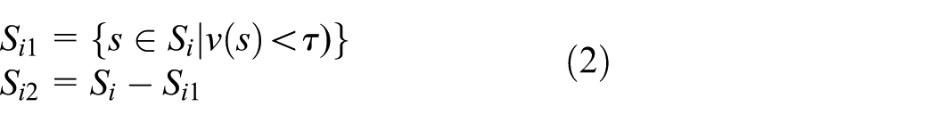
The out-of-bag (OOB) samples of a tree are the samples to be left out during the bootstrap sampling, which is approximately one-third of the training set. Each tree has its own OOB data, which can be used to evaluate the classification ability.²⁹ Therefore, we use the OOB data to test whether a tree can correctly classify these groups. The margin²⁸ is the extent to which the average of votes for the correct class exceeds the votes for the incorrect class and can be treated as the metric for measuring how accurately a tree classifies the samples. The margin of the kth tree for group g is calculated as

\begin{matrix} Margi n_{k} (X_{g}, Y_{g}) = \frac{1}{n_{k}} \cdot (\sum I (h_{k} (x) = y) \\ - \sum I (h_{k} (x) \neq y)) \end{matrix}

(3)

where ( $X_{g}$ , $Y_{g}$ ) is the set of samples of group g in the OOB data of the kth tree, (x, y) is a sample in the ( $X_{g}$ , $Y_{g}$ ), $h_{k} (\cdot)$ is the classifier of the tree, $n_{k}$ is the number of samples in ( $X_{g}$ , $Y_{g}$ ), and $I (\cdot)$ is the indicator function. The margin function measures how accurately a tree classifies samples of group g to the correct class rather than to the other class. Therefore, we calculate the voting right according to the margin. The larger the margin of the kth tree to group g, the more the confidence in the classifier of the kth tree for the samples similar to group g. If the margin of a tree for a group is negative, the tree is weak in classifying the group and should be abandoned in the voting process. Therefore, the kth tree has the voting right to group g if the margin of the kth tree to group g is greater than zero; otherwise, the tree loses the right. The voting right is represented by weight, where the value of weight is 0 or 1 and can be calculated as

\begin{matrix} weigh t_{k, g} = I (Margi n_{k} (X_{g}, Y_{g}) > 0) \end{matrix}

(4)

where $weigh t_{k, g}$ indicates whether the kth tree has the voting right to group g and $I (\cdot)$ is the indicator function. Algorithm 2 describes the process of computing the voting rights in the part-voting random-forest model.

Algorithm 2.

Calculating the voting right vector

Input: training data (SMART data)

Trees :

all decision trees in the random forest model

nTrees :

the number of trees in the random forest

Output: a weight vector and a center vector

Begin

cluster the training samples to [

g_{1}

g_{2}

,…,

g_{k}

]

centers[

c_{1}

c_{2}

,…,

c_{k}

] records the centers of [

g_{1}

g_{2}

,…,

g_{k}

]

fori in the range [

1, 2, \dots, k

] do

forj in the range [

1, 2, \dots, nTrees

] do

calculate the margin

m_{i, j}

using formula (3)

calculate the weight

w_{i, j}

using formula (4)

end for

weights = [

w_{1, 1}

w_{1, 2}

,…,

w_{1, nTrees}

[

w_{2, 1}

w_{2, 2}

,…,

w_{2, nTrees}

…

[

w_{k, 1}

w_{k, 2}

,…,

w_{k, nTrees}

]

End

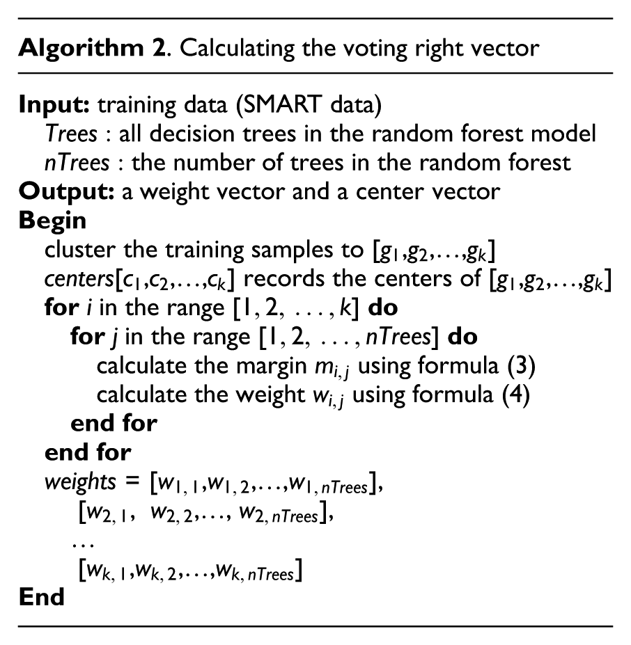
When a sample needs to be classified as “good” or “failed,” we identify its group by the similarity between the sample and the centers of groups at first; then, we use the trees that have the voting right to its group to vote on the classification result. The similarity can be computed by the Euclidean distance. The smaller the Euclidean distance, the larger the similarity; therefore, the group with the smallest distance to the sample is chosen as the similar group to the given sample. The optimization by the part-voting strategy is influenced by the accuracy of the grouping method and the number of groups. The grouping is a unsupervised classification; therefore, we explore a clustering algorithm to group the samples and choose the number of groups based on the between-cluster sum of squares by cluster.

Evaluation metrics

The FDR, FAR, accuracy, and lead time metrics are usually used to evaluate and compare the performance of failure prediction methods. The FDR is the ratio of detected soon-to-fail drives according to the prediction method to the total number of soon-to-fail drives

\begin{matrix} FDR = \frac{N_{true positive drives}}{N_{positive drives}} \end{matrix}

(5)

In the HDD failure prediction, positive drives are the soon-to-fail drives, and negative drives are the good drives. True drives are the correctly classified drives, and false drives are the incorrectly classified drives.

The FAR is the ratio of good drives detected as soon-to-fail drives by the prediction method to the total number of good drives. The number of good drives is substantially greater than that of failed drives, and a high FAR will result in significant resource waste such as increased system maintenance costs and network traffic overhead. Therefore, the FAR must be considered in the experiments

\begin{matrix} FAR = \frac{N_{false positive drives}}{N_{negative drives}} \end{matrix}

(6)

Failure prediction methods attempt to achieve the highest possible FDR with the lowest possible FAR; however, it is difficult for machine learning method to achieve both the goals.³⁰ Therefore, we use the accuracy to compare the performance of the prediction methods. The accuracy is the ratio of the number of drives that are classified correctly to the total number of drives

\begin{matrix} Accuracy = \frac{N_{true positive drives} + N_{true negative drives}}{N_{total drives}} \end{matrix}

(7)

Our prediction method needs to tune a small group of parameters. When the values of the parameters change, the chance to catch soon-to-fail drives can be increased, with increasingly more fail alarms. Therefore, we adopt the receiver operating characteristic (ROC) curve, which plots the FDR versus the FAR as the basis for the performance optimization of the method.³¹

In addition to the above-mentioned metrics, the lead time is another important metric. The lead time represents how long in advance a prediction method can alarm for impending failures. The failure prediction method needs to provide sufficient lead time for users to perform precautionary maintenance work, such as backing up data and replacing soon-to-fail drives; however, an excessive lead time is meaningless.

Experimental results

In this section, the experiments used to analyze the performance tuning and evaluation of our method are presented. Subsection “Data collection and preprocessing” describes two experimental datasets and the data preprocessing. The details of our experiments, including experimental setup, feature selection, and results comparison, are described in subsections “Experimental setup,”“Feature selection,” and “Comparative analysis,” respectively.

Data collection and preprocessing

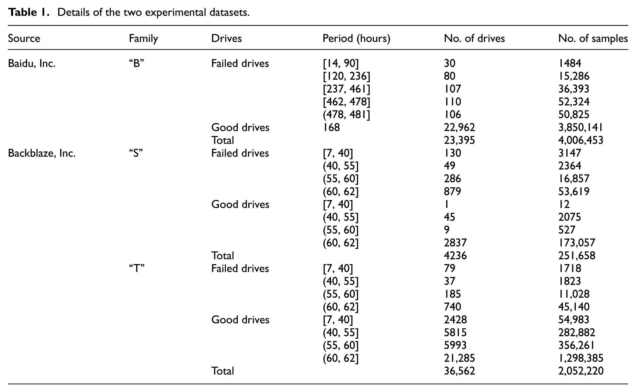
Our experimental datasets are acquired from two different sources; one dataset is from the data center of Baidu,³² and the other dataset is from the storage system of Backblaze.³³ The first dataset includes 23,395 drives of the same model, consisting of 22,962 good drives and 433 failed drives; for additional details, see Table 1. The samples in this dataset were all labeled as “good” or “failed” based on the replacement log for HDDs from the data center. A drive was labeled as “failed” if it was replaced; otherwise, it was labeled as “good.” The dataset retained 20-day SMART samples of failed drives and 7-day samples of good drives. A few drives had less than 20 days remaining in their lifetime after data collection began. These samples of drives were collected hourly. In total, there are 156,312 samples of failed drives and 3,850,141 samples of good drives.

Table 1.

Details of the two experimental datasets.

Source	Family	Drives	Period (hours)	No. of drives	No. of samples
Baidu, Inc.	“B”	Failed drives	[14, 90]	30	1484
			[120, 236]	80	15,286
			[237, 461]	107	36,393
			[462, 478]	110	52,324
			(478, 481]	106	50,825
		Good drives	168	22,962	3,850,141
		Total		23,395	4,006,453
Backblaze, Inc.	“S”	Failed drives	[7, 40]	130	3147
			(40, 55]	49	2364
			(55, 60]	286	16,857
			(60, 62]	879	53,619
		Good drives	[7, 40]	1	12
			(40, 55]	45	2075
			(55, 60]	9	527
			(60, 62]	2837	173,057
		Total		4236	251,658
	“T”	Failed drives	[7, 40]	79	1718
			(40, 55]	37	1823
			(55, 60]	185	11,028
			(60, 62]	740	45,140
		Good drives	[7, 40]	2428	54,983
			(40, 55]	5815	282,882
			(55, 60]	5993	356,261
			(60, 62]	21,285	1,298,385
		Total		36,562	2,052,220

This dataset only retained 10 SMART attributes of each sample: RSC, SUT, SER, raw read error rate (RRER), reported uncorrectable errors (RUE), high-fly writes (HFW), hardware ECC recovered (HER), current pending sector count (CPSC), POH, and TC. Each sample has 12 features: the values of all these attributes and the raw data of RSC and SPSC.

The second dataset includes 75,428 drives of over 80 models from over the course of more than 2 years, thus representing the largest public SMART dataset. The failure rate and the deterioration of HDDs are influenced by the model, manufacture, and so on;^1,22 therefore, we separate this dataset by the model of the drive in our experiments to reduce the impact of the different models. We choose two drive families with the largest number of disk drives, “ST3000DM001” and “ST4000DM000,” as our experimental dataset. To conveniently describe the experiments, these two drive families are represented as “S” and “T,” and the dataset from Baidu is represented as “B.”

The details of these two drive families are described in Table 1. A drive is labeled as “failed” if it was removed from a storage pod and replaced; otherwise, it is labeled as “good.” After removing the drives with too few health samples, family “S” includes 2892 good drives and 1344 failed drives, and family “T” includes 35,521 good drives and 1041 failed drives for our experiments. The SMART samples of these drives were typically collected for 55–62 days, and the minimum recording span was 7 days, guaranteeing that the number of samples for each drive is sufficient for our experiments. Every working drive was sampled daily. There are 75,987 samples for failed drives and 175,671 samples for good drives in family “S” and 59,709 samples for failed drives and 1,992,511 samples for good drives in family “T.”

Each sample in these datasets has 24 SMART attributes, and each attribute has a value and raw data. We removed some values and raw data that were same between good drives and failed drives and retained 16 attributes for each health sample. The retained attributes were RRER, start stop count (SSC), RSC, SER, POH, RUE, command timeout (CT), airflow temperature in celsius (ATC), load cycle count (LCC), TC, current pending sector (CPS), offline uncorrectable (OU), head flying hours (HFH), total LBAs written (TLW), and total LBAs read (TLR).

Data normalization encourages a fair comparison between the values of different features in statistical methods and machine learning algorithms by eliminating scale effects. The values and raw data of these attributes were already normalized in the first dataset when it was publicized. For the second dataset, the formula for data normalization that we used is given below

\begin{matrix} x_{N} = \frac{x - x_{\min}}{x_{\max} - x_{\min}} \end{matrix}

(8)

where x is the original value of a feature, and $x_{\min}$ and $x_{\max}$ are, respectively, the minimum and maximum of this feature in the dataset.

Compared with the dataset from Baidu, the dataset from Backblaze is larger, especially in terms of the number of failed drives and the public SMART attributes of health samples, which can more accurately evaluate the prediction results of methods. However, the dataset from Baidu is closer to the usage and deterioration of HDDs at the data center. In addition, the interval between two records in the dataset from Backblaze is 24 h, which is too long to observe the change in health samples in the degradation period before a drive fails. Therefore, we used both of these datasets as our experimental data for evaluating the prediction results of HDD failure comprehensively.

Experimental setup

To simulate the process of drive failure prediction in the real world, we use the following method to build the experiment datasets. All failed drives are randomly divided into a training set and a testing set at a ratio of 7 to 3, which guarantees that the failed drives in the training set and the testing set are completely independent. The deterioration of a failed drive is a gradual process from good to failure, and not all health samples of failed drives need to be regarded as positive samples in the training set; otherwise, those good samples of failed drives would disturb the training of the classifiers. Therefore, only the last several samples before the moment of failure of the training drives can be regarded as positive samples and need to be added to the training set; the remaining samples are useless for our experiments. The health samples of 30% of the failed drives are all added to the testing set.

For good drives, we divide up the health samples at a ratio of 7 to 3 according to their collection timelines. The earlier health samples are used in the training set. Compared with the good samples, the failed samples are rare, and our prediction method suffers from the data imbalance; therefore, we need to study how to add the good samples into the training set to achieve better prediction performance and also cover the details of good samples. This work will be described in subsection “Parameter optimization.” The latter samples are all added to the testing set to guarantee that the ratio of failed samples to good samples in the testing set matches a practical scenario.

To decide on the number of decision trees in the random forest nTree, we began the model with 20 trees. Then, we increased the number gradually in steps of 5 until the OOB error rate was stable. We used a similar procedure to choose the number of feature candidates used for the split for each node nTry, starting at the square root of the number of features and increasing with a step size of 1. Because space is limited, the detailed tuning procedure for these two parameters is not described here. They are set as follows: nTry = 6, nTree = 50 for family “B,” and nTry = 7 and nTree = 35 for families “S” and “T,” respectively. We use these settings in the following experiments.

Feature selection

It has been reported in Manousakis et al.³ and Zhu et al.¹³ that there are correlations between changes in SMART attributes and the health status of drives. We also add the change rates of values of basic features to improve the performance of the prediction method. The basic features are the values and raw data of the SMART attributes in the dataset mentioned in subsection “Data collection and preprocessing.” Several combinations of change rates with different intervals are tested in this experiment. To compare the impact of different combinations, the size of the SW is set to 1, and 70% of the earlier samples of good drives were all added to the training set, leading to a higher FAR. Unless otherwise stated, we use these settings in the following experiments.

Figure 2 shows the FDR and FAR of our method under different combinations of basic and change rate cases. In this figure, “i,j-hour” represents the combination of basic features and both i-hour and j-hour change rates. With the change of combinations, the FDR changes slightly, but the FAR changes much. For family “B,” we test 3-, 6-, 12-, and 24-h change rates of 12 basic features mentioned previously (see Figure 2(a)).

Figure 2.

FDR and FAR of different combinations of basic features and change rates: (a) family “B” and (b) family “S.”

Basic features alone achieved the highest FDR, but the FAR reached 0.083%. For the combinations of basic features and change rates of each interval, the 6-h change rates obtained the best performance, and the 3-h change rates obtained the worst performance. Due to space limitations, we do not list all the results in the figure. The prediction method with basic features and 6- and 12-h change rates achieved the highest accuracy. If 24-h change rates are included, the FDR does not change, but the FAR increased. Therefore, we add 6- and 12-h change rates as features to the dataset.

For families “S” and “T,” we first choose 8 values and 16 raw data of SMART attributes (see the first three columns in Table 2) by random forest, because random forest can assess the effects of features and automatically rank the importance of features in order.

Table 2.

Features of families “S” and “T.”

Attribute	Value	Raw data	1 day	2 days
RRER	$\sqrt$	$\sqrt$	$\sqrt$	$\sqrt$
SSC		$\sqrt$
RSC	$\sqrt$	$\sqrt$	$\sqrt$	$\sqrt$
SER	$\sqrt$	$\sqrt$	$\sqrt$	$\sqrt$
POH	$\sqrt$	$\sqrt$	$\sqrt$	$\sqrt$
PCC		$\sqrt$
RUE	$\sqrt$	$\sqrt$
CT		$\sqrt$
ATC	$\sqrt$	$\sqrt$
LCC	$\sqrt$	$\sqrt$	$\sqrt$	$\sqrt$
TC	$\sqrt$	$\sqrt$	$\sqrt$	$\sqrt$
CPS		$\sqrt$
OU		$\sqrt$
HFH		$\sqrt$	$\sqrt$	$\sqrt$
TLW		$\sqrt$	$\sqrt$	$\sqrt$
TLR		$\sqrt$	$\sqrt$	$\sqrt$

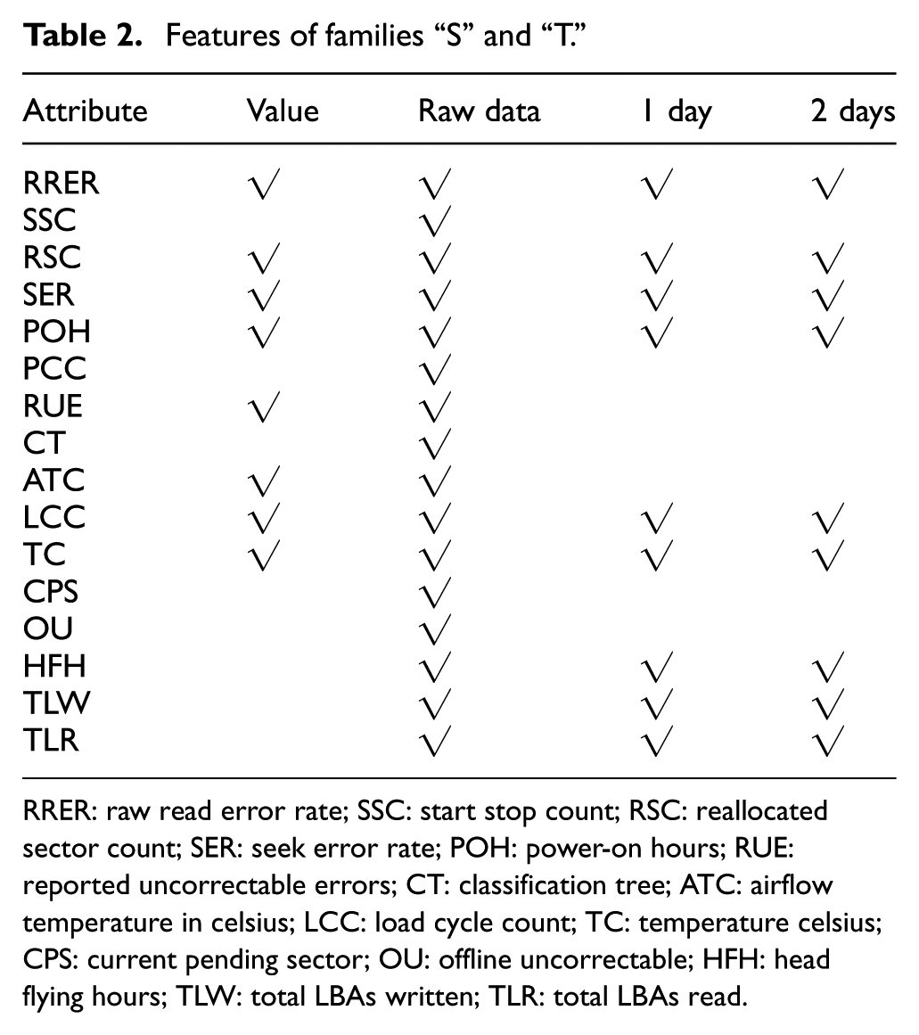
RRER: raw read error rate; SSC: start stop count; RSC: reallocated sector count; SER: seek error rate; POH: power-on hours; RUE: reported uncorrectable errors; CT: classification tree; ATC: airflow temperature in celsius; LCC: load cycle count; TC: temperature celsius; CPS: current pending sector; OU: offline uncorrectable; HFH: head flying hours; TLW: total LBAs written; TLR: total LBAs read.

Then, we test the performance of the method with the combinations of these 24 basic features and their 1-, 2-, 3-, and 4-day change rates. Figure 2(b) shows the comparison of these combinations for family “S.” The description of family “T” is omitted, because these two families obtained similar comparison results. The change in various combinations had no effect on the FDR, and the method with 1- and 2-day change rates achieved the lowest FAR. Therefore, we use the combination of basic features and 1- and 2-day change rates, which is described in Table 2.

Parameter optimization

We performed several experiments to optimize the prediction performance of our method. The experiments involved the construction of the training set, the size of SW, and the clustering of training samples.

The health status of the drives changes gradually from good to failed, and not all the health samples of failed drives need to be regarded as positive samples in the training set. Although failed drives are rare, we still only use the samples in the windows of failure (WOF) of the failed drives as positive samples rather than all of them to guarantee the validity of the positive samples in the training set. In addition, the samples of failed drives out of the WOF are abandoned. The WOF is the interval of the degradation process, that is, the time span before failure occurred.

For family “B,” we tested 12-, 24-, 36-, 48-, 96-, 168-, 216-, and 240-h WOFs and compared their effectiveness. Figure 3(a) shows the ROC comparison of different WOFs. The numbers on the colorful points are the time spans of WOFs. With larger WOFs, the FAR monotonically increases although the FDR does not increase. This is because there is a larger number of good samples of failed drives as the WOF is enlarged, and these good samples hinder the classifier training of the method. The prediction effectiveness of the 12-h WOF is worst because the 12-h WOF is too short to cover the characteristic details of HDD failures. The 216-h WOF obtained the best FDR of 98.22%, but its FAR and accuracy were 0.32% and 99.67%, respectively. The 24-h WOF obtained the best accuracy of 99.92%, the FAR was 0.065%, and the FDR was only slightly lower than that of the 216-h WOF. Therefore, we use the 24-h WOF in the following experiments for family “B.” In the similar experiment for datasets “T” and “S,” we tested 1-, 2-, 3-, and 4-day WOFs. Figure 3(b) describes the comparison of these WOFs. The method with the 1-day WOF obtained the best prediction results: an FDR of 99.1% with an FAR of 2.4%. When the WOF is enlarged, the FDR of our method remains unchanged, but the FAR increases from 2.4% to 5.8%. Therefore, we set the WOF to 1 day, which is identical to the results of family “B.”

Figure 3.

ROC comparison of different WOFs: (a) dataset “B” and (b) dataset “S.”

Only health samples in the WOF of the failed drives are added to the training set; positive samples are rare. The imbalance in the training set affects the prediction performance. We attempted to solve the problem via under-sampling, which is helpful for increasing the FDR and reducing the training overhead. However, under-sampling of negative samples increases the FAR. The smaller the ratio of good samples to bad samples in the training set, the higher the FDR and the lower the FAR, and vice versa.

We tested two sampling strategies on the negative samples: latest sampling and clustering-based sampling. Latest sampling uses the latest samples in the training set of each good drive. This idea came from a replacing strategy,¹⁵ which is a method update strategy. Clustering-based sampling clusters good samples in a training set into groups and then samples from each group. Figure 4(a) shows the FARs of 20-, 50-, and 100-group clustering with different ratios of good samples to failed samples. The 100-group clustering obtained the lowest FAR. Table 3 describes the comparison of different strategies. “All” means that 70% of the good sample is used in the training set, and the ratio of good samples to failed samples is approximately 370 for family “B.”

Figure 4.

FAR comparison of different cluster sampling methods: (a) family “B” and (b) family “T.”

Table 3.

Prediction effectiveness of training set with different sampling strategies.

Family	Strategy	Ratio of goodto failed	FDR (%)	FAR (%)
“B”	All	370	97.26	0.04
	Latest	20	99.22	0.36
		50	97.67	0.15
		100	97.67	0.06
		150	96.89	0.04
	Cluster	20	98.44	0.30
		50	97.67	0.06
		100	97.67	0.04
		150	97.67	0.017
“T”	All	1914	100	2.11
	Latest	50	100	14.8
		150	100	9.19
		250	100	9.95
		300	100	5.76
		400	100	3.11
		450	100	3.85
	Cluster	50	100	7.61
		150	100	5.43
		250	100	3.52
		300	100	1.46
		400	100	1.34
		450	100	3.16

FDR: failure detection rate; FAR: false alarm rate.

The latest strategy using a ratio of 150 can obtain a similar prediction performance with “All.” Clustering sampling obtained a lower FAR than latest sampling under the same ratios. For family “S,” good samples are roughly 130 times more than failed samples, so we did not use under-sampling. For family “T,” clustering sampling obtained the highest effectiveness (see Table 3), and the ratio of 300 to 400 and the 50-group clustering achieved the lowest FAR (see Figure 4(b)). Therefore, we chose clustering sampling and added negative samples at a rate 400 times higher than positive samples in the training set for family “T.”

We tested the influence of different SWs and thresholds on the prediction performance. Figures 5 and 6 show that the FDR and FAR can be adjusted by the SW and threshold, and the method achieves the lowest FAR (0.0087%) when the SW is set to 30–40 and the threshold is set to 1. From Figures 5 –7, we can find that there is a significant trend of decreased FDR with almost invariable FAR as the SW is enlarged, and the accuracy also decreased. Therefore, we set SW to 15 and threshold to 0.1. Figure 8 shows the mean lead time of different SWs and thresholds. The lead time is more strongly influenced by the threshold than the SW. With increasing threshold, the lead time is shortened. Fortunately, the shortest mean lead time is greater than 300 h and sufficient for users to backup data and replace the drive.

Figure 5.

FDR comparison of different SWs and thresholds.

Figure 6.

FAR comparison of different SWs and thresholds.

Figure 7.

Accuracy comparison of different SWs and thresholds.

Figure 8.

Lead time comparison of different SWs and thresholds.

We clustered the OOB samples into several groups to implement the part-voting strategy. Figure 9 describes the change in the Euclidean distance between the health samples and the last sample of a failed drive. We can see that the change in the HDD health status is non-monotonic. In family “B,” over 50% of the failed drives have a similar change trend to the plot described in Figure 9. The Euclidean distance in Figure 9 is the distance between the sample in time t and the last sample of the same drive. It is difficult to distinguish the good samples and failed samples accurately. Therefore, we only choose the last sample of the failed drives as failed sample and the first sample of the good drives as good sample. Then, if we cluster all these selected samples directly, the clustering results are of little value. To simplify and refine the samples for clustering, we use K-means algorithm to cluster good samples and failed samples, respectively. Figures 10 and 11 show the total distance within and between clusters of different degrees of clustering for good and failed samples, respectively. We chose 6 as the best number of clusters for good samples and 3 for failed samples. For families “S” and “T,” we used the above-mentioned method and set the number of clusters to the same values.

Figure 9.

Euclidean distance between the health sample and the last sample of a failed drive.

Figure 10.

Comparison of different degrees of clustering for good samples.

Figure 11.

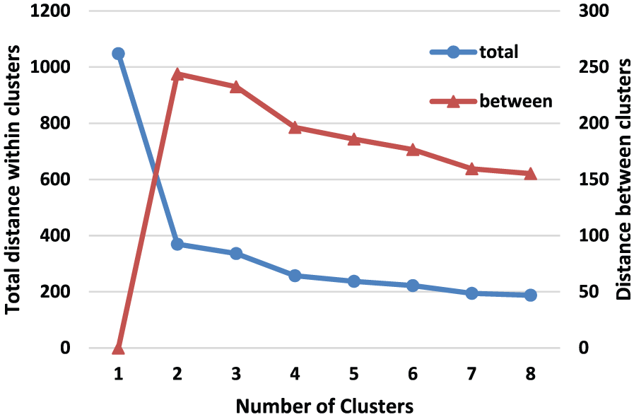
Comparison of different degrees of clustering for failed samples.

Comparative analysis

In this subsection, we compare the prediction performance of our method to the other methods mentioned in section “Background and related work” on these experimental datasets. We focus on CT, RNN, and standard random forest. The CT-based method was developed by Li et al.,¹⁵ and the RNN-based method was proposed by Xu et al.¹⁶

Figures 12 –14 show the ROC curves obtained by different methods for families “B,”“S,” and “T,” respectively. The overall performance of our method is better than CT-based method and random forest–based method on these families . On family “T,” CT-based method achieved the lower FARs. The prediction performance of CT-based method in our experiments is slightly worse than in Li et al.¹⁵ This may be caused by the following two reasons. Our experiments were developed on a different machine learning SDK, and the SMART datasets in Li et al.¹⁵ were not normalized. Random forest–based method uses the clustering-based under-sampling to keep the characteristic details of good samples in the training set, thus effectively reducing the FAR while maintaining a high FDR. Compared with RNN-based method, the FDR of RNN-based method was close to that of our method on the family “B,” but our method achieved a much lower FAR. Good drives are much more than bad drives, therefore, our method obtains higher accuracy than that of RNN-based method. On the other families, our method achieved better prediction performance than RNN-based method. In addition, RNN-based method needs a much longer training time than the other methods. CT-based method obtained the shortest training time.

Figure 12.

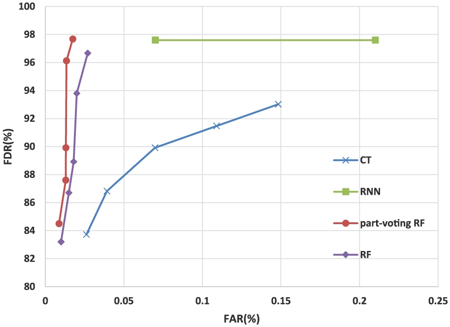
ROC comparison of CT, RNN, part-voting random forest, and random forest on family “B.”

Figure 13.

ROC comparison of CT, RNN, part-voting random forest, and random forest on family “S.”

Figure 14.

ROC comparison of CT, RNN, part-voting random forest, and random forest on family “T.”

We also compared lead times of these methods. Figure 15 shows that three methods obtained similar lead times. For these family, our method detects about 80% soon-to-fail drives 1 week ahead, which is long enough to back up data and replace them. The lead time of family “B” is longer than that of families “S” and “T,” because each drive was sampled every 24 h in families “S” and “T,” and the interval is too long.

Figure 15.

Lead time comparison of CT, RNN, and part-voting random forest.

Conclusion and future work

In this article, we presented a novel drive failure prediction method based on the part-voting random forest to improve the detection accuracy of soon-to-fail HDDs. Considering the different characteristics of each drive failure type, our method differentiates prediction of HDD failures in a coarse-grained manner by part-voting and similarity between health samples, because it is hard to classify drive failures accurately. The trees in random forest are specialized in classifying certain groups of samples rather than all samples. Therefore, the method uses a part of the decision trees that are suitable for voting on the classification result of a certain sample to improve the accuracy of the prediction. We tested the method with real-life data. The experimental results show that the random-forest-based method outperforms the other methods mentioned in section “Background and related work.” Our prediction method can achieve an FDR of 97.67% with an FAR of 0.017% for family “B,” an FDR of 100% with an FAR of 1.764% for family “S,” and an FDR of 94.89% with an FAR of 0.44% for family “T” .

There are several aspects that need to be improved. The use of SMART data to indicate impending failures is limited.³⁴ We will thus attempt to extract the workload and input/output performance of drives from system log data, and combine these data with SMART data along the time axis to facilitate classification of HDD failures and health status assessments. Moreover, we will utilize deep learning to detect the HDD failures, which can improve the accuracy of differential prediction and help users to take effective measures as early as possible.

Footnotes

Acknowledgements

The authors thank Baidu, Inc. and Backblaze, Inc. for providing the datasets used in the work.

Handling Editor: Lyudmila Mihaylova

Declaration of conflicting interests

The author(s) declared no potential conflicts of interest with respect to the research, authorship, and/or publication of this article.

Funding

The author(s) disclosed receipt of the following financial support for the research, authorship, and/or publication of this article: This work described in this paper was supported by the Fund of the Natural Science Foundation of Zhejiang Province (no. LQ17F020004), the National Key Technology R&D Program (no.2015BAH17F02), the National Natural Science Fund of China (nos 61572163, 61672200, and Y17F020150), and Hangzhou Dianzi University construction project of graduate enterprise innovation practice base (no. SJJD2014005).

References

Schroeder

Gibson

GA.

Disk failures in the real world: what does an MTTF of 1,000,000 hours mean to you? In: FAST’07 proceedings of the 5th USENIX conference on file and storage technologies, San Jose, CA, 13–16 February 2007, vol. 7, pp.1–16. Berkeley, CA: USENIX Association.

Vishwanath

Nagappan

Characterizing cloud computing hardware reliability. In: Proceedings of the 1st ACM symposium on cloud computing, Indianapolis, IN, 10–11 June 2010, pp.193–204. New York: ACM.

Manousakis

Sankar

McKnight

et al . Environmental conditions and disk reliability in free-cooled datacenters. In: 14th USENIX conference on file and storage technologies (FAST 16), Santa Clara, CA, 22–25 February 2016, pp.53–65. Berkeley, CA: USENIX Association.

Jianwei

Xingjian

Xinkui

et al . Burse: a bursty and self-similar workload generator for cloud computing. IEEE T Parall Distr 2015; 26(3): 668–680.

Douglis

et al . RAIDShield: characterizing, monitoring, and proactively protecting against disk failures. In: Proceedings of the 13th USENIX conference on file and storage technologies, Santa Clara, CA, 16–19 February 2015, pp.241–256. Berkeley, CA: USENIX Association.

Wenjun

Dianming

Yuliang

Hard drive failure prediction using big data. In: 2015 IEEE 34th symposium on reliable distributed systems workshops, Montreal, QC, Canada, 28 September–1 October 2015. New York: IEEE.

Brian

SungChang

George

et al . Hard disk drive reliability modeling and failure prediction. IEEE T Magn 2007; 43(9): 3676–3684.

Self-monitoring, analysis, and reporting technology, 2012, https://en.wikipedia.org/wiki/S.M.A.R.T.

Hungary

HDS

. Can we believe S.M.A.R.T.?Washington, DC: Technical Committee T13, Information Technology Industry Council, 2007.

10.

Kamarthi

Zeid

Bagul

. Assessment of current health of hard disk drives. In: IEEE international conference automation science engineering, Bangalore, India, 22–25 August 2009, pp.C246–C249. New York: IEEE.

11.

Murray

Hughes

Kreutz-Delgado

Machine learning methods for predicting failures in hard drives: a multiple-instance application. J Mach Learn Res 2005; 6: 783–816.

12.

Hughes

Murray

Kreutz-Delgado

et al . Improved disk-drive failure warnings. IEEE T Reliab 2002; 51(3): 350–357.

13.

Zhu

Wang

Liu

et al . Proactive drive failure prediction for large scale storage systems. In: 2013 IEEE 29th symposium on mass storage systems and technologies (MSST), Long Beach, CA, 6–10 May 2013, pp.1–5. New York: IEEE.

14.

Qian

Skelton

Moore

et al . P3: priority based proactive prediction for soon-to-fail disks. In: 2015 IEEE international conference on networking, architecture and storage (NAS), Boston, MA, 6–7 August 2015, pp.81–86. New York: IEEE.

15.

Jia

et al . Hard drive failure prediction using classification and regression trees. In: 2014 44th annual IEEE/IFIP international conference on dependable systems and networks (DSN), Atlanta, GA, 23–26 June 2014, pp.383–394. New York: IEEE.

16.

Wang

Liu

X-G

et al . Health status assessment and failure prediction for hard drives with recurrent neural networks. IEEE T Comp 2015; 13(9): 1–8.

17.

Huang

Zhang

et al . Characterizing disk failures with quantified disk degradation signatures: an early experience. In: 2015 IEEE international symposium on workload characterization (IISWC), Atlanta, GA, 4–6 October 2015, pp.150–159. New York: IEEE.

18.

Wang

Miao

Pecht

. Health monitoring of hard disk drive based on Mahalanobis distance. In: Prognostics and system health management conference (PHM-Shenzhen), Shenzhen, China, 24–25 May 2011, pp.1–8. New York: IEEE.

19.

Robnik-ikonja

MŠ.

Improving random forests. In: Boulicaut

Esposito

Giannotti

et al . (eds) Machine learning: ECML 2004. Berlin: Springer, 2004, pp.359–370.

20.

Jianwei

Collaborative recommendation with user generated content. Eng Appl Artif Intel 2015; 45: 281–294.

21.

Jianwei

Shuiguang

et al . Context-aware QoS prediction for web service recommendation and selection. Expert Syst Appl: Int J 2016; 53(C): 75–86.

22.

Pinheiro

Weber

W-D

Barroso

LA.

Failure trends in a large disk drive population. In: FAST’07 proceedings of the 5th USENIX conference on file and storage technologies, San Jose, CA, 13–16 February 2007, vol. 7, pp.17–23. Berkeley, CA: USENIX Association.

23.

Hamerly

Elkan

. Bayesian approaches to failure prediction for disk drives. In: ICML’01 proceedings of the eighteenth international conference on machine learning, Berkshires, MA, 28 June–1 July 2001, pp.202–209. San Francisco, CA: Morgan Kaufmann.

24.

Murray

Hughes

Kreutz-Delgado

Hard drive failure prediction using non-parametric statistical methods. In: ICANN/ICONIP 2003 proceedings of joint international conference on artificial neural networks and neural information processing, Istanbul, Turkey, 26–29 June 2003. Berlin, Germany: Springer.

25.

Wang

Miao

et al . Online anomaly detection for hard disk drives based on Mahalanobis distance. IEEE T Reliab 2013; 62(1): 136–145.

26.

Wang

Chow

et al . A two-step parametric method for failure prediction in hard disk drives. IEEE T Ind Inform 2014; 10(1): 419–430.

27.

Queiroz

Rodrigues

FCPR

Gomes

JPMG

et al . A fault detection method for hard disk drives based on mixture of Gaussians and nonparametric statistics. IEEE T Ind Inform 2017; 13(2): 542–550.

28.

Breiman

Random forests. Mach Learn 2001; 45(1): 5–32.

29.

Bylander

Estimating generalization error on two-class datasets using out-of-bag estimates. Mach Learn 2002; 48(1–3): 287–297.

30.

Pitakrat

van Hoorn

Grunske

. A comparison of machine learning algorithms for proactive hard disk drive failure detection. In: Proceedings of the 4th international ACM Sigsoft symposium on architecting critical systems, Vancouver, BC, Canada, 17–21 June 2013, pp.1–10. New York: ACM.

31.

Fawcett

An introduction to roc analysis. Pattern Recogn Lett 2006; 27(8): 861–874.

32.

Smart data set from Nankai University and Baidu, Inc., http://pan.baidu.com/share/link?shareid=189977&uk=4278294944 (2013, accessed 1 January 2015).

33.

Hard drive data and stats from Backblaze, Inc., https://www.backblaze.com/b2/hard-drive-test-data.html (2016, accessed 1 July 2016).

34.

Sankar

Shaw

Vaid

. Impact of temperature on hard disk drive reliability in large datacenters. In: 2011 IEEE/IFIP 41st international conference on dependable systems & networks (DSN), Hong Kong, China, 27–30 June 2011, pp.530–537. New York: IEEE.

Random-forest-based failure prediction for hard disk drives

Abstract

Keywords

Introduction

Background and related work

HDD failure

SMART

SMART-based HDD failure prediction

Prediction method based on part-voting random forest

Random-forest-based HDD failure prediction

Part-voting strategy

Evaluation metrics

Experimental results

Data collection and preprocessing

Experimental setup

Feature selection

Parameter optimization

Comparative analysis

Conclusion and future work

Footnotes

Acknowledgements

Declaration of conflicting interests

Funding

References