Fault diagnosis method for closed-loop satellite attitude control systems based on a fuzzy parity equation

Abstract

This article proposes a fault diagnosis method for closed-loop satellite attitude control systems based on a fuzzy model and parity equation. The fault in a closed-loop system is propagated with the feedback loop, increasing the difficulty of fault diagnosis and isolation. The study uses a Takagi-Sugeno (T-S) fuzzy model and parity equation to diagnose and isolate a fault in a closed-loop satellite attitude control system. A fully decoupled parity equation is designed for the closed-loop satellite attitude control system to generate a residual that is sensitive only to a specific actuator and sensor. A T-S fuzzy model is used to describe the nonlinear closed-loop satellite attitude control system. With the combination of the T-S fuzzy model and fully decoupled parity equation, the fuzzy parity equation (FPE) of the nonlinear system can be obtained. Then this article uses a parameter estimator based on a Kalman filter to identify deviations and scale factor changes from information contained in the residuals generated by the FPE. The actuator and sensor fault detection and isolation simulation of the three-axis stable satellite attitude control system is provided for illustration.

Introduction

The closed-loop satellite attitude control system (CLSACS) is the most critical subsystem guaranteeing the normal operation of a satellite. However, it has a complex structure, a poor working environment, unknown disturbances and uncertain factors. Furthermore, it is one of the most fault-prone subsystems. For satellites in orbit, an attitude control system fault often leads to disaster and is likely to result in satellite roll and attitude loss within a short period, ultimately causing satellite mission failure.^1–7 Because the faulty satellite component is irreparable, fault-tolerant control methods for the CLSACS must be investigated, and the operational status of the CLSACS must be effectively monitored. Timely detection of a fault in the CLSACS and the implementation of effective fault-tolerant controls can improve the reliability and security of satellites and also reduce risk. Incorporation of reconfigurable or safety controls can protect the CLSACS from catastrophic accidents as well as enhance the resilience of the system.^8,9

Traditional fault diagnosis methods primarily consider open-loop systems, and there are currently no in-depth studies of fault diagnosis for closed-loop systems in the literature. Although Adnane et al. ¹⁰ demonstrate a new design version of the extended Kalman filter which is effective and can be utilized as an alternative LEO satellite attitude estimation system, the study did not consider the sensor fault propagation problem in closed-loop systems. Zhou et al. ¹¹ proposed two main reasons for a decline in fault diagnosis performance. First, as the introduction of a feedback system generally makes a system more robust to external disturbances, the impact of the control variable may be overshadowed when a fault is in its early stages or of a smaller amplitude. The residual signal may still be within a range of small fluctuations when a fault occurs, making fault detection difficult and increasing the loss detection rate. Second, feedback control may propagate faults within a system, resulting in abnormal signals. For example, in an open-loop system, a sensor fault occurring in the system will not affect other sensors because the measurement signal is still within the normal range, while in a closed-loop system, with a feedback signal introduced, the use of an abnormal measured value by the feedback controller may cause the control signal to deviate from the normal trend and subsequently cause the entire system to depart from the normal operating range. In this case, the signals measured by other sensors are also abnormal. Overall, fault propagation increases the difficulty of fault isolation. Research and analysis related to closed-loop diagnosis are important aspects of fault-tolerant control for a closed-loop system, which improves the robustness of the system. Yang and Zhang ¹² achieved fault detection and isolation for a closed-loop system by constructing a double observer. However, the observer gain matrix design was complex, the computational burden was large, and the fault diagnosis performance was poor. Ruschmann et al. ¹³ used fuzzy parity equations (FPE) to diagnose the faults of actuators and sensors in flight control systems and estimated the relevant fault parameters, though faults in closed-loop systems were neither estimated nor analysed. Cheng et al. ¹⁴ proposed a combined method for detecting and isolating minor actuator faults in closed-loop control systems, yet they did not analyse the propagation of faults in a closed-loop system. Wu and Liu ¹⁵ diagnosed the fault in the pitch actuator of wind turbines with the method that combined the interval prediction algorithm with the recursive subspace identification based on the variable forgetting factor algorithm. Because the fault in the pitch actuator will propagate in the closed-loop system, the method cannot diagnose the fault in the closed-system.

This article examines the system time redundancy and principles of fault propagation in closed-loop systems and then establishes a set of fully decoupled parity equations (FDPEs) for fault diagnosis of actuators and sensors.

This study presents a fault diagnosis that incorporates both FDPEs and the Takagi-Sugeno (T-S) model, a method in which the residual is sensitive to a specific fault and is decoupled from system states, disturbance inputs and other faults. The design methods of the FDPEs for the fault control system (actuator faults, sensor faults and multiple faults) is discussed; the fault model is estimated through parameter estimation using residual information; and the simulations of detection, isolation and identification of actuator, sensor and multiple faults are accomplished.

CLSACS dynamics model

The CLSACS is a typical closed-loop control system. A fault in a member of a closed-loop system spreads with the closed-loop feedback, and detection and isolation are difficult to achieve.^16,17 In this study, a rigid three-axis stabilized satellite is considered.

The satellite actuator consists of three orthogonal flywheels, and the measuring device is a combination of star sensors and gyros. The three-axis stabilized satellite attitude dynamics equations are as follows ¹⁸

$$\{\begin{array}{c}{I}_{\mathrm{x}}{\stackrel{·}{\omega }}_x+\left(J_{\mathrm{z}}-J_{\mathrm{y}}\right){\omega }_y{\omega }_z=-T_{cx}+H_y{\omega }_z-H_z{\omega }_y+T_{dx}\\ I_{\mathrm{y}}{\stackrel{·}{\omega }}_y+\left(J_{\mathrm{x}}-J_{\mathrm{z}}\right){\omega }_z{\omega }_x=-T_{cy}+H_z{\omega }_x-H_x{\omega }_z+T_{dy}\\ I_{\mathrm{z}}{\stackrel{·}{\omega }}_z+\left(J_{\mathrm{y}}-J_{\mathrm{x}}\right){\omega }_x{\omega }_y=-T_{cz}+H_x{\omega }_y-H_y{\omega }_x+T_{dz}\end{array}$$

(1)

where ${\omega }_x,{\omega }_y,{\omega }_z$ denote the three angular velocities of the satellite; $H_x,H_y,H_z$ , the moment angular momentum; $T_{\mathrm{dx}},T_{\mathrm{dy}},T_{\mathrm{dz}}$ , the space environmental disturbance torques; $T_{\mathrm{cx}},T_{\mathrm{cy}},T_{c\mathrm{z}}$ , the control torques; and $I_x,I_y,I_z$ , the satellite inertia moments.

Assume that the rotational speed of the satellite orbit system with respect to the inertial system is $(0,-{\omega }_0,0)$ . The three attitude angles of the satellite with respect to the tracking system are the roll angle $\phi$ , pitch angle $\theta$ and yaw angle $\psi$ . The rotation angular velocity of the satellite relative to the orbital coordinate system is $[\begin{array}{ccc}\hfill \stackrel{·}{\phi }\hfill & \hfill \stackrel{·}{\theta }\hfill & \hfill \stackrel{·}{\psi }\hfill \end{array}]$ .

When the three attitude angles are small, the conversion matrix for converting from the satellite orbit coordinate system to the body axes coordinate system is

$$C_{\mathrm{BO}}=\left[\begin{array}{ccc}\hfill 1\hfill & \hfill \psi \hfill & \hfill -\theta \hfill \\ \multicolumn{1}{c}{-\psi }& \hfill 1\hfill & \hfill \phi \hfill \\ \multicolumn{1}{c}{\theta }& \hfill -\phi \hfill & \hfill 1\hfill \end{array}\right]$$

(2)

Then, ${\omega }_x,{\omega }_y,{\omega }_z$ can be expressed as

$$\left[\begin{array}{c}\hfill {\omega }_x\hfill \\ \multicolumn{1}{c}{{\omega }_y}\\ \multicolumn{1}{c}{{\omega }_z}\end{array}\right]=\left[\begin{array}{c}\hfill \stackrel{·}{\varphi }\hfill \\ \multicolumn{1}{c}{\stackrel{·}{\theta }}\\ \multicolumn{1}{c}{\stackrel{·}{\psi }}\end{array}\right]+\left[\begin{array}{ccc}\hfill 1\hfill & \hfill \psi \hfill & \hfill -\theta \hfill \\ \multicolumn{1}{c}{-\psi }& \hfill 1\hfill & \hfill \varphi \hfill \\ \multicolumn{1}{c}{\theta }& \hfill -\varphi \hfill & \hfill 1\hfill \end{array}\right]\left[\begin{array}{c}\hfill 0\hfill \\ \multicolumn{1}{c}{-{\omega }_0}\\ \multicolumn{1}{c}{0}\end{array}\right]=\left[\begin{array}{c}\hfill \stackrel{·}{\varphi }-{\omega }_0\psi \hfill \\ \multicolumn{1}{c}{\stackrel{·}{\theta }-{\omega }_0}\\ \multicolumn{1}{c}{\stackrel{·}{\psi }+{\omega }_0\varphi }\end{array}\right]$$

(3)

After applying differential calculus to equation (3), we obtain

$$\left[\begin{array}{c}\hfill {\stackrel{·}{\omega }}_x\hfill \\ \multicolumn{1}{c}{{\stackrel{·}{\omega }}_y}\\ \multicolumn{1}{c}{{\stackrel{·}{\omega }}_z}\end{array}\right]=\left[\begin{array}{c}\hfill \stackrel{··}{\varphi }-{\omega }_0\stackrel{·}{\psi }\hfill \\ \multicolumn{1}{c}{\stackrel{··}{\theta }}\\ \multicolumn{1}{c}{\stackrel{··}{\psi }+{\omega }_0\stackrel{·}{\varphi }}\end{array}\right]$$

(4)

Without considering other disturbance torques, the space environmental disturbance torques can be expressed as follows when the three attitude angles are small

$$\{\begin{array}{c}\hfill T_{\mathrm{dx}}\approx 3{\omega }_0^2(I_z-I_y)\varphi \hfill \\ \multicolumn{1}{c}{T_{d\mathrm{y}}\approx 3{\omega }_0^2(I_z-I_x)\theta }\\ \multicolumn{1}{c}{T_{\mathrm{dz}}\approx 0}\end{array}$$

(5)

Substituting equations (4) and (5) into equation (1), we obtain

$$\{\begin{array}{c}\hfill I_x\stackrel{··}{\varphi }+[{\omega }_0^2(4I_y-4I_z)-{\omega }_0{H}_y]\varphi +(-{\omega }_0{I}_x+{\omega }_0{I}_y-{\omega }_0{I}_z-H_y)\stackrel{·}{\psi }+H_z\stackrel{·}{\theta }+(I_z-I_y)\stackrel{·}{\theta }\stackrel{·}{\psi }+{\omega }_0(I_z-I_y)\stackrel{·}{\theta }\varphi =-T_{\mathrm{cx}}+{\omega }_0{H}_z\hfill \\ \multicolumn{1}{c}{I_y\stackrel{··}{\theta }+3{\omega }_0^2(I_x-I_z)\theta -H_z\stackrel{·}{\varphi }+{\omega }_0{H}_z\psi +H_x\stackrel{·}{\psi }+{\omega }_0{H}_x\varphi +(I_x-I_z)(\stackrel{·}{\psi }\stackrel{·}{\varphi }+{\omega }_0\varphi \stackrel{·}{\varphi }-{\omega }_0^2\psi \varphi -{\omega }_0\psi \stackrel{·}{\psi })=-T_{\mathrm{cy}}}\\ \multicolumn{1}{c}{I_z\stackrel{··}{\psi }+[{\omega }_0^2(-I_x+I_y)-{\omega }_0{H}_y]\psi +({\omega }_0{I}_x-{\omega }_0{I}_y+{\omega }_0{I}_z+H_y)\stackrel{·}{\varphi }-H_x\stackrel{·}{\theta }+(I_y-I_x)(\stackrel{·}{\varphi }\stackrel{·}{\theta }-{\omega }_0\psi \stackrel{·}{\theta })=-T_{\mathrm{cz}}-{\omega }_0{H}_x}\end{array}$$

(6)

The controller chosen for the CLSACS is the proportional derivative control. The control torques are

$$\{\begin{array}{c}\hfill T_{\mathrm{cx}}=K_x({\tau }_x\stackrel{·}{\phi }+\phi )\hfill \\ \multicolumn{1}{c}{T_{\mathrm{cy}}=K_y({\tau }_y\stackrel{·}{\theta }+\theta )}\\ \multicolumn{1}{c}{T_{\mathrm{cz}}=K_z({\tau }_z\stackrel{·}{\psi }+\psi )}\end{array}$$

(7)

where $K_x,K_y,K_z$ denote the proportionality coefficients of the controller and ${\tau }_x,{\tau }_y,{\tau }_z$ , the differential coefficients of the controller.

The state variable $x=[\begin{array}{cccccc}\hfill \phi \hfill & \hfill \stackrel{·}{\phi }\hfill & \hfill \theta \hfill & \hfill \stackrel{·}{\theta }\hfill & \hfill \psi \hfill & \hfill \stackrel{·}{\psi }\hfill \end{array}{]}^T$ , and the measurement equation is

$$y=\mathrm{Cx}+v$$

(8)

where $C=\left[\begin{array}{cccccc}\hfill 1\hfill & \hfill 0\hfill & \hfill 0\hfill & \hfill 0\hfill & \hfill 0\hfill & \hfill 0\hfill \\ \multicolumn{1}{c}{0}& \hfill 1\hfill & \hfill 0\hfill & \hfill 0\hfill & \hfill -{\omega }_0\hfill & \hfill 0\hfill \\ \multicolumn{1}{c}{0}& \hfill 0\hfill & \hfill 1\hfill & \hfill 0\hfill & \hfill 0\hfill & \hfill 0\hfill \\ \multicolumn{1}{c}{0}& \hfill 0\hfill & \hfill 0\hfill & \hfill 1\hfill & \hfill 0\hfill & \hfill 0\hfill \\ \multicolumn{1}{c}{0}& \hfill 0\hfill & \hfill 0\hfill & \hfill 0\hfill & \hfill 1\hfill & \hfill 0\hfill \\ \multicolumn{1}{c}{{\omega }_0}& \hfill 0\hfill & \hfill 0\hfill & \hfill 0\hfill & \hfill 0\hfill & \hfill 1\hfill \end{array}\right]$ and v is white noise.

If the state variable of the CLSACS is the same as in equation (8), the CLSACS can be expressed as follows according to equation (6)

$$\stackrel{·}{x}=f\left(x\right)+\mathrm{Bu}+w$$

(9)

where $x\in R^{n\times 1}$ denotes the system state variable, $u\in R^{p\times 1}$ , the system input variable; $f(x)$ is a smooth nonlinear function and $w\in R^n$ denotes the system white noise.

Suppose that the working point of the CLSACS is $o(o=1,2,\dots ,P)$ , where P denotes the number of working points. Then, the linearized model of the system equation at o can be approximately expressed as

$$\{\begin{array}{c}\hfill x_o(k+1)=A_o{x}_o\left(k\right)+B_{o}u\left(k\right)+w\left(k\right)\hfill \\ \multicolumn{1}{c}{y\left(k\right)=C_o{x}_o\left(k\right)+v\left(k\right)}\end{array}$$

(10)

where $A_o=(I+Y_M\mathrm{\Delta }t+Y_M^2\mathrm{\Delta }{t}^2)/2$ , I is a unit matrix $6\times 6$ , $\mathrm{\Delta }t$ denotes the sampling period, $Y_M=(\partial f(x))/(\partial x_o(k))$ is a Jacobian matrix and $C_o=C$ .

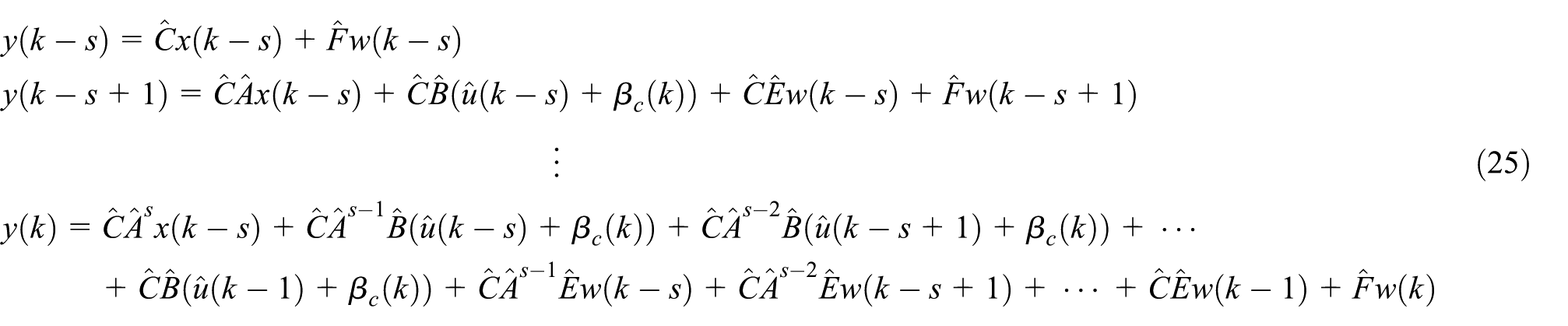
The satellite attitude control system (equation (6)) is a nonlinear system, whereas the parity equation is suitable only for linear systems. El-Amrani et al. ¹⁹ introduced the T-S model to describe a nonlinear system to improve diagnostic accuracy.

A CLSACS can be expressed as a T-S fuzzy control system constructed such that the three attitude angles $\mathrm{\Phi }=(\begin{array}{ccc}\hfill \phi \hfill & \hfill \theta \hfill & \hfill \psi \hfill \end{array})$ function as the premise variable. Each working point corresponds to a fuzzy rule. ²⁰

Rule $o(o=1,2,\dots ,P)$ : If $\mathrm{\Phi }$ is $M_o(M_o=(\begin{array}{ccc}\hfill {\phi }_o\hfill & \hfill {\theta }_o\hfill & \hfill {\psi }_o\hfill \end{array}))$ , then the locally linear model of a CLSACS can be expressed as equation (10) at the working point o. ²⁰

The global model of the CLSACS state equation can be expressed as

$$x(k+1)=\frac{\sum _{o=1}^P{\xi }_o\left(\mathrm{\Phi }\right)[A_o{x}_o\left(k\right)+B_o{u}_o\left(k\right)+w_o\left(k\right)]}{\sum _{o=1}^P{\xi }_o\left(\mathrm{\Phi }\right)}$$

(11)

where ${\xi }_o(\mathrm{\Phi })$ is the membership degree, which is determined by the premise variable according to the membership function, ${\xi }_o(\mathrm{\Phi })=\underset{j=1}{\overset{P}{\Pi }}{\mu }_{\mathrm{oj}}(\mathrm{\Phi })$ , $\mathrm{\Phi }$ is function of time variable k.

Fault propagation analysis of a closed-loop system

To effectively diagnose the faults of a control system, it is necessary to understand the propagation of faults in a closed-loop system and analyse the impact of faults in the system. The approach taken in this study is to first define the discrete equations of the system and then add feedback; faults are then added to the actuators and sensors. Finally, the propagation of the actuator and sensor faults in the closed-loop system is diagnosed.

The discrete equations of the control system are

$$\{\begin{array}{c}\hfill x(k+1)=\mathrm{Ax}\left(k\right)+\mathrm{Bu}\left(k\right)+\mathrm{Ew}\left(k\right)\hfill \\ \multicolumn{1}{c}{y\left(k\right)=\mathrm{Cx}\left(k\right)+\mathrm{Fw}\left(k\right)}\end{array}$$

(12)

where $x(k)\in R^{n\times 1}$ denotes the system state variable; $y(k)\in R^{q\times 1}$ , the system output variable; $u(k)\in R^{p\times 1}$ , the actuator input; $w(k)\in R^{r\times 1}$ , the system disturbance; and $A,B,C,E,F$ are matrices with the appropriate dimensions.

We add a feedback loop to equation (12). Output feedback is a common type of feedback control method. ²¹ Thus, we consider output feedback as the feedback loop

$$u_{\mathrm{cN}}\left(k\right)=u\prime \left(k\right)+\mathrm{Ky}\left(k\right)=u\prime \left(k\right)+\mathrm{KCx}\left(k\right)+\mathrm{KFw}\left(k\right)$$

(13)

where $u\prime (k)$ is the system input.

After substituting (13) into (12), we obtain

$$\begin{array}{c}\multicolumn{1}{c}{x(k+1)=\mathrm{Ax}\left(k\right)+\mathrm{Bu}\left(k\right)+\mathrm{Ew}\left(k\right)}\\ =(A+\mathrm{BKC})x\left(k\right)+\mathrm{Bu}\prime \left(k\right)+(\mathrm{BKF}+E)w\left(k\right)\hfill \end{array}$$

(14)

which is the control system state equation with feedback.

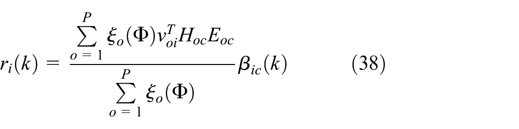
According to Wang and Xiong, ²² the fault models of actuators and sensors are considered as

$$\{\begin{array}{c}\hfill u_c\left(k\right)=u_{\mathrm{cN}}\left(k\right)+{\beta }_c\hfill \\ \multicolumn{1}{c}{y_s\left(k\right)=y_{\mathrm{sN}}\left(k\right)+{\beta }_s}\end{array}$$

(15)

where $u_c$ is the actual actuator input, $u_{\mathrm{cN}}$ is the ideal actuator input, $y_s$ is the actual sensor input, $y_{\mathrm{cN}}$ is the ideal sensor input, ${\beta }_c$ is the actuator deviation fault, ${\beta }_s$ is the sensor deviation fault, and ${\beta }_c$ and ${\beta }_s$ can be abrupt or time-varying faults.

Next, the propagation of actuator and sensor faults in a closed-loop system is analysed based on the closed-loop system model and fault model.

• 1. Actuator fault propagation

When an actuator is faulty and ${\beta }_s=0$ , based on equation (13), the actuator can be expressed as

$$u_c\left(k\right)=u_{\mathrm{cN}}\left(k\right)+{\beta }_c=u\prime \left(k\right)+\mathrm{KCx}\left(k\right)+\mathrm{KFw}\left(k\right)+{\beta }_c$$

(16)

By substituting equation (16) into equation (12), the system state equation can be rewritten as

$$\begin{array}{c}\multicolumn{1}{c}{x(k+1)=\mathrm{Ax}\left(k\right)+B{u}_c\left(k\right)+\mathrm{Ew}\left(k\right)}\\ \multicolumn{1}{c}{=(A+\mathrm{BKC})x\left(k\right)}\\ +B[u\prime \left(k\right)+{\beta }_c]+(\mathrm{BKF}+E)w\left(k\right)\hfill \end{array}$$

(17)

When an actuator is faulty, the form of the fault can be expressed as in equation (17), and the coefficient matrix of the fault is the same as the control matrix of the given instruction.

According to equations (12) and (17), the effect of an actuator fault on the sensor output is expressed as

$$\begin{array}{c}y(k+1)=\mathrm{Cx}(k+1)+\mathrm{Fw}(k+1)\hfill \\ =C(A+\mathrm{BKC})x\left(k\right)+\mathrm{CB}[u\prime \left(k\right)+{\beta }_c]\hfill \\ +C(E+\mathrm{BKF})w(k+1)+\mathrm{Fw}(k+1)\hfill \end{array}$$

(18)

As noted above, an actuator fault affects both the system state and system measurement output.

• 2. Sensor fault propagation

When a sensor is faulty and ${\beta }_c=0$ , by combining equations (12) and (15), we can obtain the measured output of the system as

$$y_s\left(k\right)=y_{\mathrm{sN}}\left(k\right)+{\beta }_s=\mathrm{Cx}\left(k\right)+\mathrm{Fw}\left(k\right)+{\beta }_s$$

(19)

Due to the existence of the output feedback loop, the fault of a sensor will be propagated with the feedback loop and then affect the instruction input of the control system actuator. The instruction input of the control system can be expressed as

$$u\left(k\right)=u\prime \left(k\right)+\mathrm{Ky}\left(k\right)=u\prime \left(k\right)+\mathrm{KCx}\left(k\right)+\mathrm{KFw}\left(k\right)+K{\beta }_s$$

(20)

When the control instruction acts on the system state equation and the sensor is faulty, the system state equation is

$$\begin{array}{c}\multicolumn{1}{c}{x(k+1)=\mathrm{Ax}\left(k\right)+B{u}_s\left(k\right)+\mathrm{Ew}\left(k\right)}\\ \multicolumn{1}{c}{=(A+\mathrm{BKC})x\left(k\right)+B[u\prime \left(k\right)+K{\beta }_s]}\\ +(E+\mathrm{BKF})w\left(k\right)\hfill \end{array}$$

(21)

The above analysis illustrates that a sensor fault can be propagated with the feedback loop, affecting the system input and the system state equation. A sensor fault also affects the output of measurement and disturbs the actuator input, and thus fault isolation is affected. Regarding the actuator input and system state, the coefficient matrix of the fault parameter ${\beta }_s$ , including the feedback matrix K, indicates that the effect of a sensor fault on a system is related to the design of the feedback matrix K.

Fault diagnosis of an actuator in a closed-loop system

FPE for the fault diagnosis of an actuator

After we establish the FDPE and obtain the residual error generated by the FDPE, the residual state equation can be obtained by using the T-S model, which means the method of FPE. The residual error is estimated by using a Kalman filter based on the equation of the residual. The estimated residual error can be compared with the set threshold to determine whether an actuator is faulty.

The fault model representing the case in which the $i\mathrm{th}$ actuator is faulty is shown in equation (15). Assume that the fault of the actuator does not change within a data window, so

$${\beta }_c\left(k\right)={\left[\begin{array}{ccccc}\hfill 0\hfill & \hfill \cdots \hfill & \hfill {\beta }_{\mathrm{ic}}\left(k\right)\hfill & \hfill \cdots \hfill & \hfill 0\hfill \end{array}\right]}^T(i=1,2,\dots ,p)$$

where p is the dimension for a given input $u\prime (k)$ and ${\beta }_{\mathrm{ic}}(k)$ is the fault parameter of the ith actuator. Thus, the system equation at time $k-s$ is as follows

$$\{\begin{array}{c}y(k-s)=\mathrm{Cx}(k-s)+\mathrm{Fw}(k-s)\hfill \\ \multicolumn{1}{c}{u(k-s)=u\prime (k-s)+\mathrm{Ky}(k-s)+{\beta }_c\left(k\right)=u\prime (k-s)+\mathrm{KCx}(k-s)+\mathrm{KFw}(k-s)+{\beta }_c\left(k\right)}\\ \multicolumn{1}{c}{x(k-s+1)=\mathrm{Ax}(k-s)+\mathrm{Bu}(k-s)+\mathrm{Ew}(k-s)=(A+\mathrm{BKC})x(k-s)+B(u\prime (k-s)+{\beta }_c\left(k\right))+(\mathrm{BKF}+E)w(k-s)}\end{array}$$

(22)

At time $k-s+1$ , the system measurement equation is

$$\begin{array}{c}y(k-s+1)=\mathrm{Cx}(k-s+1)+\mathrm{Fw}(k-s+1)\hfill \\ =C(A+\mathrm{BKC})x(k-s)+\mathrm{CB}(u\prime (k-s)+{\beta }_c\left(k\right))\hfill \\ +C(\mathrm{BKF}+E)w(k-s)+\mathrm{Fw}(k-s+1)\hfill \end{array}$$

(23)

Then, the measurement equation at time k is

$$\begin{array}{c}\multicolumn{1}{c}{y\left(k\right)=\mathrm{Cx}\left(k\right)+\mathrm{Fw}\left(k\right)}\\ \multicolumn{1}{c}{=C{(A+\mathrm{BKC})}^{s}x(k-s)}\\ +C{(A+\mathrm{BKC})}^{s-1}B(u\prime (k-s)+{\beta }_c\left(k\right))\hfill \\ +C{(A+\mathrm{BKC})}^{s-2}B(u\prime (k-s+1)+{\beta }_c\left(k\right))\hfill \\ +\cdots +\mathrm{CB}(u\prime (k-1)+{\beta }_c\left(k\right))\hfill \\ +C{(A+\mathrm{BKC})}^{s-1}(\mathrm{BKF}+E)w(k-s)\hfill \\ +C{(A+\mathrm{BKC})}^{s-2}(\mathrm{BKF}+E)w(k-s+1)\hfill \\ +\cdots +C(\mathrm{BKF}+E)w(k-1)+\mathrm{Fw}\left(k\right)\hfill \end{array}$$

(24)

Let $\hat{A}=A+\mathrm{BKC}$ , $\hat{B}=B$ , $\hat{E}=\mathrm{BKF}+E$ , $\hat{C}=C$ , $\hat{F}=F$ and $\hat{u}(k)=u\prime (k)$ , and assume that the data window length is $s+1$ . Then, from time $k-s$ to time k, the observation data $y(k-s),\dots ,y(k)$ satisfy

$$\begin{array}{c}y(k-s)=\hat{C}x(k-s)+\hat{F}w(k-s)\hfill \\ y(k-s+1)=\hat{C}\hat{A}x(k-s)+\hat{C}\hat{B}(\hat{u}(k-s)+{\beta }_c\left(k\right))+\hat{C}\hat{E}w(k-s)+\hat{F}w(k-s+1)\hfill \\ ⋮\hfill \\ y\left(k\right)=\hat{C}{\hat{A}}^{s}x(k-s)+\hat{C}{\hat{A}}^{s-1}\hat{B}(\hat{u}(k-s)+{\beta }_c\left(k\right))+\hat{C}{\hat{A}}^{s-2}\hat{B}(\hat{u}(k-s+1)+{\beta }_c\left(k\right))+\cdots \hfill \\ +\hat{C}\hat{B}(\hat{u}(k-1)+{\beta }_c\left(k\right))+\hat{C}{\hat{A}}^{s-1}\hat{E}w(k-s)+\hat{C}{\hat{A}}^{s-2}\hat{E}w(k-s+1)+\cdots +\hat{C}\hat{E}w(k-1)+\hat{F}w\left(k\right)\hfill \end{array}$$

(25)

Equation (25) can be expressed as

$$Y\left(k\right)=H_{0}x(k-s)+H_c(U_N\left(k\right)+{\beta }_c^{*}\left(k\right))+H_{w}W\left(k\right)$$

(26)

where $Y(k)=[y^T(k-s)\cdots y^T(k){]}^T$ denotes the measured quantity; $U_N(k)=[{\hat{u}}^T(k-s)\cdots {\hat{u}}^T(k){]}^T$ , the actuator input; $W(k)=[w^T(k-s)\cdots w^T(k){]}^T$ , the disturbance input; ${\beta }_c^{*}(k)=[\begin{array}{ccc}\hfill {{\beta }_c}^T(k)\hfill & \hfill \cdots \hfill & \hfill {{\beta }_c}^T(k)\hfill \end{array}{]}^T$ , the actuator fault parameter vector; and $H_0$ , $H_c$ and $H_w$ , the redundant measurement matrix, where

$$H_0=\left[\begin{array}{c}\widehat{C}\\ \widehat{C}\widehat{A}\\ ⋮\\ \widehat{C}{\widehat{A}}^s\end{array}\right]$$

(27)

$$\begin{array}{c}\multicolumn{1}{c}{H_c=\left[\begin{array}{cccccc}\hfill 0\hfill & \hfill 0\hfill & \hfill \hfill & \hfill \cdots \hfill & \hfill \hfill & \hfill 0\hfill \\ \multicolumn{1}{c}{\hat{C}\hat{B}}& \hfill 0\hfill & \hfill 0\hfill & \hfill \cdots \hfill & \hfill \hfill & \hfill 0\hfill \\ \multicolumn{1}{c}{\hat{C}\hat{A}\hat{B}}& \hfill \hat{C}\hat{B}\hfill & \hfill 0\hfill & \hfill 0\hfill & \hfill \cdots \hfill & \hfill 0\hfill \\ \multicolumn{1}{c}{⋮}& \hfill \hfill & \hfill \hat{C}\hat{B}\hfill & \hfill 0\hfill & \hfill 0\hfill & \hfill 0\hfill \\ \multicolumn{1}{c}{\hat{C}{\hat{A}}^{s-2}\hat{B}}& \hfill \cdots \hfill & \hfill \hfill & \hfill \hat{C}\hat{B}\hfill & \hfill 0\hfill & \hfill 0\hfill \\ \multicolumn{1}{c}{\hat{C}{\hat{A}}^{s-1}\hat{B}}& \hfill \hat{C}{\hat{A}}^{s-2}\hat{B}\hfill & \hfill \cdots \hfill & \hfill \hat{C}\hat{A}\hat{B}\hfill & \hfill \hat{C}\hat{B}\hfill & \hfill 0\hfill \end{array}\right],}\\ \multicolumn{1}{c}{H_w=\left[\begin{array}{cccccc}\hfill \hat{F}\hfill & \hfill 0\hfill & \hfill \hfill & \hfill \cdots \hfill & \hfill \hfill & \hfill 0\hfill \\ \multicolumn{1}{c}{\hat{C}\hat{E}}& \hfill \hat{F}\hfill & \hfill 0\hfill & \hfill \cdots \hfill & \hfill \hfill & \hfill 0\hfill \\ \multicolumn{1}{c}{\hat{C}\hat{A}\hat{E}}& \hfill \hat{C}\hat{E}\hfill & \hfill \hat{F}\hfill & \hfill 0\hfill & \hfill \cdots \hfill & \hfill 0\hfill \\ \multicolumn{1}{c}{⋮}& \hfill \hfill & \hfill \hat{C}\hat{E}\hfill & \hfill \hat{F}\hfill & \hfill 0\hfill & \hfill 0\hfill \\ \multicolumn{1}{c}{\hat{C}{\hat{A}}^{s-2}\hat{E}}& \hfill \cdots \hfill & \hfill \hfill & \hfill \hat{C}\hat{E}\hfill & \hfill \hat{F}\hfill & \hfill 0\hfill \\ \multicolumn{1}{c}{\hat{C}{\hat{A}}^{s-1}\hat{E}}& \hfill \hat{C}{\hat{A}}^{s-2}\hat{E}\hfill & \hfill \cdots \hfill & \hfill \hat{C}\hat{A}\hat{E}\hfill & \hfill \hat{C}\hat{E}\hfill & \hfill \hat{F}\hfill \end{array}\right]}\end{array}$$

(28)

Based on Song et al., ²³ we construct a fully decoupled parity vector (FDPV), denoted as $v_i^T$ , that is sensitive only to the $i\mathrm{th}$ actuator and satisfies

$$v_i^T\left[\begin{array}{ccc}\hfill H_0\hfill & \hfill H_w\hfill & \hfill H_{\mathrm{ci}}\hfill \end{array}\right]=0$$

(29)

where

$$H_{\mathrm{ci}}=\left[\begin{array}{cccccc}\hfill 0\hfill & \hfill 0\hfill & \hfill \hfill & \hfill \cdots \hfill & \hfill \hfill & \hfill 0\hfill \\ \multicolumn{1}{c}{\hat{C}{\hat{B}}^{*}}& \hfill 0\hfill & \hfill 0\hfill & \hfill \cdots \hfill & \hfill \hfill & \hfill 0\hfill \\ \multicolumn{1}{c}{\hat{C}\hat{A}{\hat{B}}^{*}}& \hfill \hat{C}{\hat{B}}^{*}\hfill & \hfill 0\hfill & \hfill 0\hfill & \hfill \cdots \hfill & \hfill 0\hfill \\ \multicolumn{1}{c}{⋮}& \hfill \hfill & \hfill \hat{C}{\hat{B}}^{*}\hfill & \hfill 0\hfill & \hfill 0\hfill & \hfill 0\hfill \\ \multicolumn{1}{c}{\hat{C}{\hat{A}}^{s-2}{\hat{B}}^{*}}& \hfill \cdots \hfill & \hfill \hfill & \hfill \hat{C}{\hat{B}}^{*}\hfill & \hfill 0\hfill & \hfill 0\hfill \\ \multicolumn{1}{c}{\hat{C}{\hat{A}}^{s-1}{\hat{B}}^{*}}& \hfill \hat{C}{\hat{A}}^{s-2}{\hat{B}}^{*}\hfill & \hfill \cdots \hfill & \hfill \hat{C}\hat{A}{\hat{B}}^{*}\hfill & \hfill \hat{C}{\hat{B}}^{*}\hfill & \hfill 0\hfill \end{array}\right]$$

(30)

${\hat{B}}^{*}$ is $\hat{B}$ without the $i\mathrm{th}$ column which corresponds to actuator i, that is, the actuator to which the parity equations are applied. For example, for the first actuator, ${\hat{B}}^{*}=[\begin{array}{cccc}\hfill b_2\hfill & \hfill b_3\hfill & \hfill \cdots \hfill & \hfill b_p\hfill \end{array}]$ , where $b_l(l=1,2,\dots p)$ is the column vector of $\hat{B}$ .

Consider each row of $v_i$ as $v_{i,s}$ , then the following notation for $v_i$ can be obtained

$$v_i=\left[\begin{array}{c}\hfill v_{i,1}\hfill \\ \multicolumn{1}{c}{v_{i,2}}\\ \multicolumn{1}{c}{⋮}\\ \multicolumn{1}{c}{v_{i,s}}\end{array}\right]$$

Then, we can get $v_i^T=[\begin{array}{cccc}\hfill v_{i,1}\hfill & \hfill v_{i,2}\hfill & \hfill \cdots \hfill & \hfill v_{i,s}\hfill \end{array}],v_{i,s}\in R$ .

The $v_i^T$ computed according equations (27)–(30) is now only sensitive to the $i\mathrm{th}$ actuator and not sensitive to the other actuators and system disturbances. Thus, the residual error is affected by actuator i and is decoupled from the other actuators and disturbances. When an actuator is faulty, only the corresponding residual error is nonzero, thus, fault isolation is achieved.

The necessary and sufficient condition for the existence of the nonzero $v_i^T$ of equation (29) is

$$s>\frac{N_c}{q}-1$$

(31)

where $N_c$ is the number of columns that are not related to matrix $\left[\begin{array}{ccc}\hfill H_0\hfill & \hfill H_w\hfill & \hfill H_{\mathrm{ci}}\hfill \end{array}\right]$ and q denotes the dimension of the output variable.

The FDPE residual $r_i(k)$ , which is sensitive only to the $i\mathrm{th}$ actuator, is defined as

$$r_i\left(k\right)=v_i^T[Y\left(k\right)-H_c{U}_N\left(k\right)]$$

(32)

where $U_N(k)=[u{\prime }^T(k-s)\cdots u{\prime }^T(k){]}^T$ denotes the actuator input.

By substituting equation (26) into equation (32), residual $r_i(k)$ can be rewritten as

$$\begin{array}{c}\multicolumn{1}{c}{r_i\left(k\right)=v_i^T[H_{0}x(k-s)+H_c(U_N\left(k\right)+{\beta }_c^{*})+H_{w}W\left(k\right)-H_c{U}_N\left(k\right)]}\\ =v_i^T[H_{0}x(k-s)+H_c{\beta }_c^{*}+H_{w}W\left(k\right)]\hfill \end{array}$$

(33)

Equation (26) indicates that $v_i^T$ satisfies $v_i^T{H}_0=0$ and $v_i^T{H}_w=0$ , meaning that the FDPV is decoupled from both the system state and disturbance. Therefore, the residual $r_i(k)$ can be expressed as

$$r_i\left(k\right)=v_i^T{H}_c{\beta }_c^{*}\left(k\right)$$

(34)

Because the designed FDPV is sensitive to the $i\mathrm{th}$ actuator but decoupled from the other actuators, only the fault of the first actuator should be considered in the fault diagnosis. We assume that

$${\beta }_c^{*}\left(k\right)={\beta }_{\mathrm{ic}}\left(k\right)·E_c$$

(35)

where $E_c=[\begin{array}{ccc}\hfill 1\hfill & \hfill \cdots \hfill & \hfill 1\hfill \end{array}{]}^T$ is a $(s+1)p$ column vector and ${\beta }_{\mathrm{ic}}(k)$ denotes the fault parameter of the $i\mathrm{th}$ actuator.

By substituting equation (35) into equation (34), the parity equation residual $r_i(k)$ can be rewritten as

$$r_i\left(k\right)=v_i^T{H}_c{E}_c{\beta }_{\mathrm{ic}}\left(k\right)$$

(36)

The above discussion indicates that ${\beta }_{\mathrm{ic}}(k)=0$ and $r_i(k)=0$ when the actuator is normal and that ${\beta }_{\mathrm{ic}}(k)\ne 0$ and $r_i(k)\ne 0$ when the actuator is faulty; $v_i^T$ should satisfy

$$v_i^T{H}_c\ne 0$$

(37)

Otherwise, the FDPE residual will always be zero and cannot reflect the fault characteristics. When $v_i^T$ is selected, it should increase the value of $v_i^T{H}_c{E}_c{\beta }_{\mathrm{ic}}(k)$ , ensuring that the projection of the fault feature in the direction of $v_i^T$ can be fully reflected. Otherwise, the fault characteristic information can be easily overwhelmed by noise, which cannot be detected by the FDPE.

By applying the T-S model presented in the section ‘CLSACS dynamics model’, we can express the output of the T-S model as

$$r_i\left(k\right)=\frac{\sum _{o=1}^P{\xi }_o\left(\mathrm{\Phi }\right)v_{\mathrm{oi}}^T{H}_{\mathrm{oc}}{E}_{\mathrm{oc}}}{\sum _{o=1}^P{\xi }_o\left(\mathrm{\Phi }\right)}{\beta }_{\mathrm{ic}}\left(k\right)$$

(38)

where ${\xi }_o(\mathrm{\Phi })=\underset{j=1}{\overset{p}{\Pi }}{\mu }_{\mathrm{oj}}(\mathrm{\Phi })$ .

The correspondence between the fault parameters and the residual error is used as the observation equation. Thus, we obtain

$$r_i\left(k\right)=\varphi \left(k\right){\beta }_{\mathrm{ic}}\left(k\right)+\eta \left(k\right)$$

(39)

where

$$\varphi \left(k\right)=\frac{\sum _{o=1}^P{\xi }_o\left(\mathrm{\Phi }\right)v_{\mathrm{oi}}^T{H}_{\mathrm{oc}}{E}_{\mathrm{oc}}}{\sum _{o=1}^P{\xi }_o\left(\mathrm{\Phi }\right)}$$

and $\eta (k)$ is the zero-mean white noise with a covariance matrix of $R(k)$ .

Because the change trend of ${\beta }_{\mathrm{ic}}(k)$ is unknown, the dynamic model is set up as a random walk process

$${\beta }_{\mathrm{ic}}(k+1)={\beta }_{\mathrm{ic}}\left(k\right)+\epsilon \left(k\right)$$

(40)

where $\epsilon (k)$ is the independent zero-mean white noise with a covariance matrix of $Q(k)$ .

The actuator fault parameter ${\beta }_{\mathrm{ic}}(k)$ is estimated by using a Kalman filter according to equations (39) and (40).

The fault parameters are statistically determined, and the fault threshold is $T_{\mathrm{CD}}$ . If $|{\beta }_{\mathrm{ic}}(k)|>T_{\mathrm{CD}}$ , the actuator is faulty; if $|{\beta }_{\mathrm{ic}}(k)|<T_{\mathrm{CD}}$ , the actuator operates correctly.

The fault diagnosis of an actuator in a closed-loop system is completed. When multiple actuators are faulty, multiple actuator fault diagnoses and isolations can be achieved. Then, the fault parameters can be estimated after establishing the FDPE for each actuator.

Simulation results and analysis

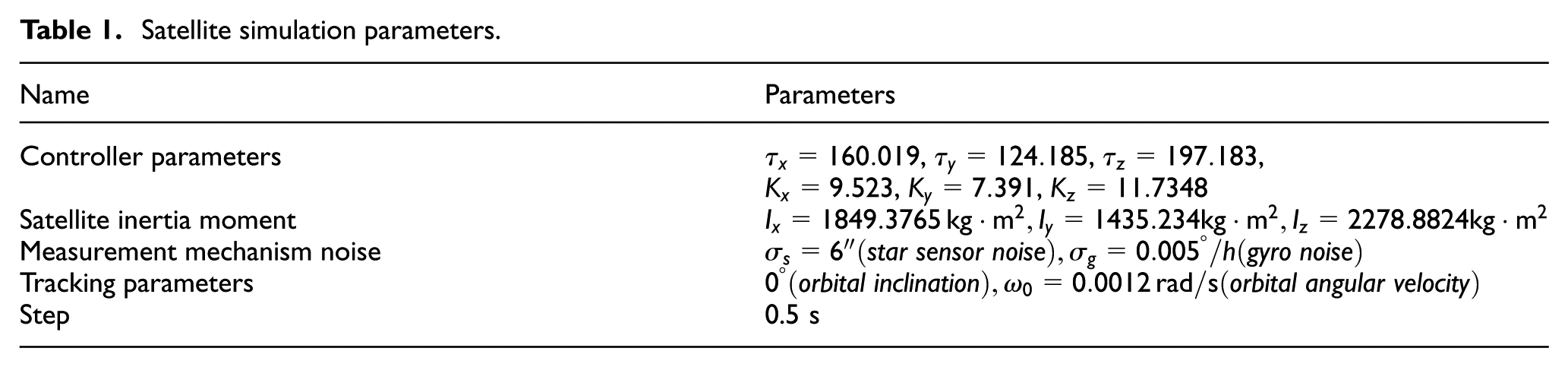
The actuator fault of a three-axis stabilized CLSACS is simulated. The output feedback loop and controller are designed simultaneously. The controller is replaced with the output feedback loop to ensure the stable operation of the system. The parameters which are provided by the team’s predecessors are shown in Table 1.

Table 1.

Satellite simulation parameters.

Name	Parameters
Controller parameters	${\tau }_x=160.019$ , ${\tau }_y=124.185$ , ${\tau }_z=197.183$ , $K_x=9.523$ , $K_y=7.391$ , $K_z=11.7348$
Satellite inertia moment	$I_x=1849.3765\mathrm{kg}·{\mathrm{m}}^2,I_y=1435.234\mathrm{kg}·{\mathrm{m}}^2,I_z=2278.8824\mathrm{kg}·{\mathrm{m}}^2$
Measurement mechanism noise	${\sigma }_s=6″\left(\mathrm{star}\mathrm{sensor}\mathrm{noise}\right),{\sigma }_g=0.{005}^{\circ }/h\left(\mathrm{gyro}\mathrm{noise}\right)$
Tracking parameters	$0^{\circ }\left(\mathrm{orbital}\mathrm{inclination}\right),{\omega }_0=0.0012\mathrm{rad}/\mathrm{s}\left(\mathrm{orbital}\mathrm{angular}\mathrm{velocity}\right)$
Step	0.5 s

When the CLSACS is described, the triangle membership function is chosen for the premise variables. The working point and membership function are selected as shown in Figure 1.

Figure 1.

Schematic of the working point selection and membership function of the antecedent variables.

An abrupt fault at the Y-axis actuator is expressed as

$${\beta }_{ic}=\{\begin{array}{l}0t<600\mathrm{s}\hfill \\ 2\times {10}^{-3}t\ge 600\mathrm{s}\hfill \end{array}$$

(41)

After establishing the fully decoupled fuzzy parity equation (FDFPE) for the three-axis actuator of a control system, the fault parameter can be estimated as follows.

Figures 2 and 3 illustrate that when the FDFPE is established for the Z-axis actuator, the fault deviation estimation result is a zero-mean sequence that is affected only by noise. For the Y-axis, the FDFPE is established to estimate the true fault error. Some errors exist in the estimation results before or after the time at which the fault is added; for the remainder of the time, the fault parameter can be estimated accurately. Thus, the FDFPE is effective in the detection and isolation of actuator faults.

Figure 2.

Y-axis actuator deviation estimation result.

Figure 3.

Z-axis actuator deviation estimation result.

A time-varying fault at the Y-axis actuator is expressed as

$${\beta }_{\mathrm{ic}}=\{\begin{array}{cc}0\hfill & \hfill t<600\mathrm{s}\hfill \\ \multicolumn{1}{c}{1.5\times {10}^{-6}\times (t-600)}& \hfill t\ge 600\mathrm{s}\hfill \end{array}$$

(42)

In the same manner, after establishing the FDFPE for the three-axis actuator of a control system, the fault parameter can be estimated as follows.

Figures 4 and 5 show that when the actuator fault is time varying, the fault parameter can be accurately estimated after the FDFPE for the system is established. Thus, fault detection and isolation can be completed, and the goal of the actuator fault detection and isolation can be achieved.

Figure 4.

Residual of the Y-axis actuator.

Figure 5.

Residual of the Z-axis actuator.

To verify the ability of the FDFPE to diagnose the faults of multiple actuators, at 600 s, the abrupt fault shown in equation (41) is added to the X-axis, and the time-varying fault shown in equation (42) is added to the Y-axis. After establishing the FDFPE for the three-axis actuator of the control system, the fault parameters can be estimated as follows.

Figures 6–8 show that when multiple actuators are faulty, the FPEs established for different actuators reflect only the fault characteristics of the corresponding actuator. The fault parameters can be estimated using the residual error information of the parity equation and the Kalman filter. Identification of the fault parameters can result in the detection and isolation of the system fault.

Figure 6.

Residual of the X-axis actuator.

Figure 7.

Residual of the Y-axis actuator

Figure 8.

Residual of the Z-axis actuator.

Fault diagnosis of a sensor in a closed-loop system

FPE for the fault diagnosis of a sensor

When a sensor is faulty, the fault not only will directly affect the measurement results of the sensor but can also propagate through the feedback loop in a closed-loop system, thereby affecting the input of the actuator and system state. The FPE for the fault diagnosis of a sensor is established based on the same method presented in the ‘Fault diagnosis of an actuator in a closed-loop system’ section. A double parity equation diagnosis method is designed based on the propagation characteristics of a sensor fault in a closed-loop system. A set of parity equations is used for fault detection and isolation, and another set is used to estimate the fault parameters.

The fault model representing the case in which the $i\mathrm{th}$ sensor is faulty is shown in equation (15). Assume that the fault deviation of the same sensor does not change within a data window and the fault vectors ${\beta }_s(k)=[\begin{array}{ccccc}\hfill 0\hfill & \hfill \cdots \hfill & \hfill {\beta }_{\mathrm{si}}(k)\hfill & \hfill \cdots \hfill & \hfill 0\hfill \end{array}{]}^T(i=1,2,\dots ,q)$ , where q is the dimension of output $y(k)$ and ${\beta }_{\mathrm{si}}(k)$ is the fault parameter of the $i\mathrm{th}$ sensor. The system equation at time $k-s$ is as follows

$$\{\begin{array}{c}y(k-s)=\mathrm{Cx}(k-s)+\mathrm{Fw}(k-s)+{\beta }_s\left(k\right)\hfill \\ \multicolumn{1}{c}{u(k-s)=u\prime (k-s)+\mathrm{Ky}(k-s)=u\prime (k-s)+\mathrm{KCx}(k-s)+\mathrm{KFw}(k-s)+K{\beta }_s\left(k\right)}\\ \multicolumn{1}{c}{x(k-s+1)=\mathrm{Ax}(k-s)+\mathrm{Bu}(k-s)+\mathrm{Ew}(k-s)=(A+\mathrm{BKC})x(k-s)+B(u\prime (k-s)+K{\beta }_s\left(k\right))+(\mathrm{BKF}+E)w(k-s)}\end{array}$$

(43)

At time $k-s+1$ , the system measurement equation is

$$\begin{array}{c}y(k-s+1)=\mathrm{Cx}(k-s+1)+\mathrm{Fw}(k-s+1)+{\beta }_s\left(k\right)\hfill \\ =C(A+\mathrm{BKC})x(k-s)+\mathrm{CB}(u\prime (k-s)+K{\beta }_s\left(k\right))\hfill \\ +C(\mathrm{BKF}+E)w(k-s)+\mathrm{Fw}(k-s+1)+{\beta }_s\left(k\right)\hfill \end{array}$$

(44)

Hence, the measurement equation at time k is

$$\begin{array}{c}y\left(k\right)=\mathrm{Cx}\left(k\right)+\mathrm{Fw}\left(k\right)+{\beta }_s\left(k\right)\hfill \\ =C{(A+\mathrm{BKC})}^{s}x(k-s)+C{(A+\mathrm{BKC})}^{s-1}B(u\prime (k-s)+K{\beta }_s\left(k\right))+C{(A+\mathrm{BKC})}^{s-2}B(u\prime (k-s+1)+K{\beta }_s\left(k\right))\hfill \\ +\cdots +\mathrm{CB}(u\prime (k-1)+K{\beta }_s\left(k\right))+C{(A+\mathrm{BKC})}^{s-1}(\mathrm{BKF}+E)w(k-s)\hfill \\ +C{(A+\mathrm{BKC})}^{s-2}(\mathrm{BKF}+E)w(k-s+1)+\cdots +C(\mathrm{BKF}+E)w(k-1)+\mathrm{Fw}\left(k\right)+{\beta }_s\left(k\right)\hfill \end{array}$$

(45)

With the same method in the ‘Fault diagnosis of an actuator in a closed-loop system’ section, the equation (46) is computed as follows

$$Y\left(k\right)=H_{0}x(k-s)+H_c(U_N\left(k\right)+\mathrm{\Gamma })+H_{w}W\left(k\right)+{\beta }_s^{*}\left(k\right)$$

(46)

where $Y(k)=[y^T(k-s)\cdots y^T(k){]}^T$ , $U_N(k)=[{\hat{u}}^T(k-s)\cdots {\hat{u}}^T(k){]}^T$ , $W(k)=[w^T(k-s)\cdots w^T(k){]}^T$ , ${\beta }_s^{*}(k)=[\begin{array}{ccc}\hfill {{\beta }_s}^T(k)\hfill & \hfill \cdots \hfill & \hfill {{\beta }_s}^T(k)\hfill \end{array}{]}^T$ is the sensor fault parameter vector, and $\mathrm{\Gamma }(k)=[\begin{array}{ccc}\hfill {(K{\beta }_s(k))}^T\hfill & \hfill \cdots \hfill & \hfill {(K{\beta }_s(k))}^T\hfill \end{array}{]}^T$ is the function vector of the sensor fault with the feedback loop with respect to the system state. $H_0$ , $H_c$ and $H_w$ are the same as in section ‘Fault diagnosis of an actuator in a closed-loop system’.

Li et al. ²¹ introduced a method for constructing the FDPEs of a sensor, which works well in open-loop systems. However, because of the existence of the feedback loop, a sensor fault in closed-loop systems can degrade the actuator; as the time redundancy measurement equation is related only to a specific sensor, the sensor fault cannot be obtained.

Some scholars have suggested enhancing the fault information in the residual of the parity equation by optimizing the design of the feedback controller of the closed-loop system. ¹¹ Following their work, the double parity equation diagnosis method is designed based on the propagation characteristics of a sensor fault in a closed-loop system. A set of parity equations is used to detect and isolate the fault, and another set is used to estimate the fault parameters.

• 1. Parity equations for fault detection and isolation

The FDPV $v_{\mathrm{di}}^T$ , which is used for sensor fault detection and isolation, should satisfy

$$v_{\mathrm{di}}^T\left[\begin{array}{ccc}\hfill H_0\hfill & \hfill H_w\hfill & \hfill H_c\hfill \end{array}\right]=0$$

(47)

Equation (47) can ensure that the parity equation is decoupled from the system state, system disturbance and feedback vector $\mathrm{\Gamma }(k)$ .

After the FDPVs are constructed, the parity equation residual $r_{\mathrm{di}}(k)$ can be expressed as

$$r_{\mathrm{di}}\left(k\right)=v_{\mathrm{di}}^T[Y\left(k\right)-H_c{U}_N\left(k\right)]$$

(48)

By substituting equation (46) into equation (48), we obtain

$$\begin{array}{c}{r}_{\mathrm{di}}\left(k\right)=v_{\mathrm{di}}^T[H_{0}x(k-s)+H_c(U_N\left(k\right)+\mathrm{\Gamma }\left(k\right))+H_{w}W\left(k\right)+{\beta }_s^{*}\left(k\right)-H_c{U}_N\left(k\right)]\hfill \\ =v_{\mathrm{di}}^T[H_{0}x(k-s)+H_c\mathrm{\Gamma }+H_{w}W\left(k\right)+{\beta }_s^{*}\left(k\right)]\hfill \end{array}$$

(49)

Based on equation (47), the parity equation residual $r_{\mathrm{di}}(k)$ can be simplified to

$$r_{\mathrm{di}}\left(k\right)=v_{\mathrm{di}}^T{\beta }_s^{*}\left(k\right)$$

(50)

In this manner, the residual error $r_d(k)$ related only to the parity equation is obtained. However, this error can only be used to detect the fault; the location of the fault is not determined, and fault isolation is not completed.

When only the $i\mathrm{th}$ sensor is faulty, ${\beta }_s(k)=[\begin{array}{ccccc}\hfill 0\hfill & \hfill \cdots \hfill & \hfill {\beta }_{\mathrm{si}}(k)\hfill & \hfill \cdots \hfill & \hfill 0\hfill \end{array}{]}^T(i=1,2,\dots ,p)$ and ${\beta }_s^{*}=[\begin{array}{ccc}\hfill {{\beta }_s}^T\hfill & \hfill \cdots \hfill & \hfill {{\beta }_s}^T\hfill \end{array}{]}^T$ . Decoupling matrix $\mathrm{\Lambda }$ is constructed to satisfy

$${\beta }_s^{*}\left(k\right)=\mathrm{\Lambda }{\beta }_s\left(k\right)$$

(51)

where $\mathrm{\Lambda }$ is $((s+1)p)\times ((s+1)p)$ . The diagonal elements of $\mathrm{\Lambda }$ in the diagonal of $(j-1)p+i(j=1,2,\dots ,s+1,i=1,2,\dots ,p)$ are 1, which corresponds to the fault parameters of the $i\mathrm{th}$ sensor, whereas the remaining elements of $\mathrm{\Lambda }$ are 0.

For example, let $s=3$ and $p=6$ , if the matrix $\mathrm{\Lambda }$ is corresponding to the first sensor fault. Then, $\mathrm{\Lambda }=\mathrm{diag}[\begin{array}{cccccccc}\hfill 1\hfill & \hfill 0\hfill & \hfill \cdots \hfill & \hfill 0\hfill & \hfill 1\hfill & \hfill 0\hfill & \hfill \cdots \hfill & \hfill 0\hfill \end{array}]$ , with the 1st, 7th, 13th and 19th diagonal elements of $\mathrm{\Lambda }$ being equal to 1, which reflects the fault position of the first faulty sensors in ${\beta }_s^{*}$ .

Let $v_{\mathrm{di}}^T$ satisfy

$$v_{\mathrm{di}}^T\mathrm{\Lambda }=0$$

(52)

Then, the parity equation residual can be expressed as

$$r_{\mathrm{di}}\left(k\right)=v_{\mathrm{di}}^T{\beta }_s^{*}\left(k\right)=v_{\mathrm{di}}^T\mathrm{\Lambda }{\beta }_s^{*}\left(k\right)=0$$

(53)

$v_{\mathrm{di}}^T$ , which satisfies equation (52), is only decoupled from the $i\mathrm{th}$ sensor fault and is sensitive to the remaining sensor faults.

Considering the effect of noise, the fault parameters are statistically determined, and the fault threshold is $T_{\mathrm{SD}}$ . If $|r_{\mathrm{di}}(k)|<T_{\mathrm{SD}}$ , the parity equation residual includes fault information. If $|r_{\mathrm{di}}(k)|>T_{\mathrm{SD}}$ , the parity equation residual does not include fault information.

When only one sensor is faulty, after designing multiple FDPVs that are decoupled from each sensor in the aforementioned manner, we can determine that a sensor parity equation residual equal to zero represents a fault. If multiple sensors are faulty, the FDPV can be constructed such that many diagonal elements of $\mathrm{\Lambda }$ are equal to 1. Then, the faults can be detected and isolated by using the parity equation residual.

Because $v_{\mathrm{di}}^T$ is designed to be decoupled from the redundant measurement matrices $H_0$ , $H_c$ and $H_w$ and the decoupling matrix $\mathrm{\Lambda }$ , the degrees of freedom of the FDPV design are reduced, and the projection of the fault in the direction of $v_{\mathrm{di}}^T$ can be less noticeable. An FDPV with a high sensitivity to faults should be selected to improve the diagnostic reliability.

• 2. Parity equation for fault parameter estimation

If the observation equation for the Kalman filter is constructed based on equation (54), the fault parameter will be an $(s+1)p$ -dimensional state variable, and the computational burden will be large.

To reduce the computational burden of the filter estimation, another FDPV, denoted as $v_{\mathrm{ei}}^T$ , is designed to estimate the fault parameter.

The $v_{\mathrm{ei}}^T$ that satisfies equation (47) is constructed; the corresponding parity equation residual can then be expressed as

$$r_{\mathrm{ei}}\left(k\right)=v_{\mathrm{ei}}^T{\beta }_s^{*}\left(k\right)$$

(54)

where $r_{\mathrm{ei}}(k)$ is a one-dimensional vector and ${\beta }_s^{*}(k)$ is multidimensional. The computational burden of the filter estimation is reduced by reducing the dimensions of the fault parameters. The location of the fault sensor in ${\beta }_s^{*}(k)$ can be determined based on fault isolation. In the case of a single fault mode, the fault parameters corresponding to faulty sensor ${\beta }_s^{*}(k)$ are nonzero, and the remaining elements of ${\beta }_s^{*}(k)$ are 0.

Assume that the sensor fault does not change within a data window.

A new fault parameter vector is composed of the fault parameters of the $i\mathrm{th}$ sensor in ${\beta }_s^{*}(k)$

$${\beta }_{\mathrm{es}}^{*}\left(k\right)=E^{*}{\beta }_{\mathrm{si}}\left(k\right)$$

(55)

where $E^{*}=[\begin{array}{ccc}\hfill 1\hfill & \hfill \cdots \hfill & \hfill 1\hfill \end{array}{]}^T$ is an $s+1$ -dimensional vector, all the elements of which are equal to 1.

Considering fault parameter vector ${\beta }_s^{*}(k)$ , only the fault parameters corresponding to the faulty sensor are nonzero. When the $i\mathrm{th}$ sensor is faulty, the value of the new FDPV $v_{\mathrm{ei}}^{*T}$ corresponds to the position of the $i\mathrm{th}$ sensor fault for $v_{\mathrm{ei}}^T$ .

The other elements of $v_{\mathrm{ei}}^{*T}$ are multiplied by the zero element of ${\beta }_s^{*}(k)$ and thus do not affect the result of the residual. Therefore, equation (50) can be expressed as

$$r_{\mathrm{ei}}\left(k\right)=v_{\mathrm{ei}}^{*T}{\beta }_{\mathrm{es}}^{*}\left(k\right)=v_{\mathrm{ei}}^{*T}{E}^{*}{\beta }_{\mathrm{si}}\left(k\right)$$

(56)

Equation (50) illustrates that the unknown fault parameter changed is ${\beta }_s^{*}(k)$ , which is a one-dimensional scalar. Thus, the dimension of the estimated state is reduced.

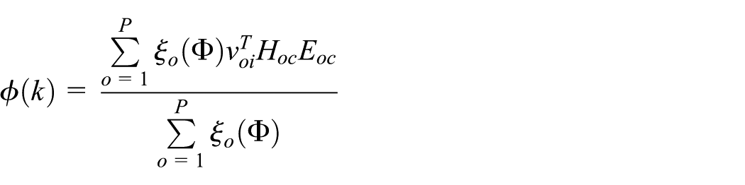
Based on the T-S model presented in the ‘CLSACS dynamics model’ section, we obtain

$$r_i\left(k\right)=\frac{\sum _{o=1}^P{\xi }_o\left(\mathrm{\Phi }\right)v_{\mathrm{ei}}^{*T}{E}^{*}}{\sum _{o=1}^P{\xi }_o\left(\mathrm{\Phi }\right)}{\beta }_{\mathrm{si}}\left(k\right)$$

(57)

We can estimate the fault parameter via the optimal estimation method. Assume that measurement noise $\eta (k)$ is a zero-mean white-noise covariance matrix, that is, $R(k)$ . Then, we obtain

$$r_{\mathrm{ei}}\left(k\right)={\varphi }_{\mathrm{ei}}\left(k\right){\beta }_{\mathrm{si}}\left(k\right)+\eta \left(k\right)$$

(58)

where

$${\varphi }_{\mathrm{ei}}\left(k\right)=\frac{\sum _{o=1}^P{\xi }_o\left(\mathrm{\Phi }\right)v_{\mathrm{ei}}^{*T}{E}^{*}}{\sum _{o=1}^P{\xi }_o\left(\mathrm{\Phi }\right)}$$

The dynamic model is set up as a random walk process because the change trend of ${\beta }_{\mathrm{si}}(k)$ is unknown

$${\beta }_{\mathrm{si}}(k+1)={\beta }_{\mathrm{si}}\left(k\right)+\epsilon \left(k\right)$$

(59)

where $\epsilon (k)$ is the independent zero-mean white noise and $Q(k)$ is the covariance matrix. The fault parameter ${\beta }_{\mathrm{si}}(k)$ can be estimated using the Kalman filter according to equations (58) and (59).

The method for reducing the dimensions of a sensor’s fault parameters is suitable only when a single sensor is at fault. Equation (56) cannot be obtained when multiple sensors are at fault.

Simulation results and analysis

The first sensor fault in the CLSACS is simulated and verified. The simulation parameters are shown in Table 1.

An abrupt fault at the first sensor is expressed as follows

$${\beta }_{si}=\{\begin{array}{l}0t<600\mathrm{s}\hfill \\ 2\times {10}^{-3}t\ge 600\mathrm{s}\hfill \end{array}$$

(60)

Based on the time redundancy measurement information, the FPE is established according to equations (54) and (50) to diagnose the sensor fault.

Select simulation results are shown below (a 5-s smoothing window is applied to the residual results).

Figures 9 and 10 illustrate that if the sensor that the residual is decoupled from is the faulty sensor, the residual will be the sequence that is affected only by noise. If the sensor that the residual is decoupled from is not the faulty sensor, the fault will be reflected in the residual.

Figure 9.

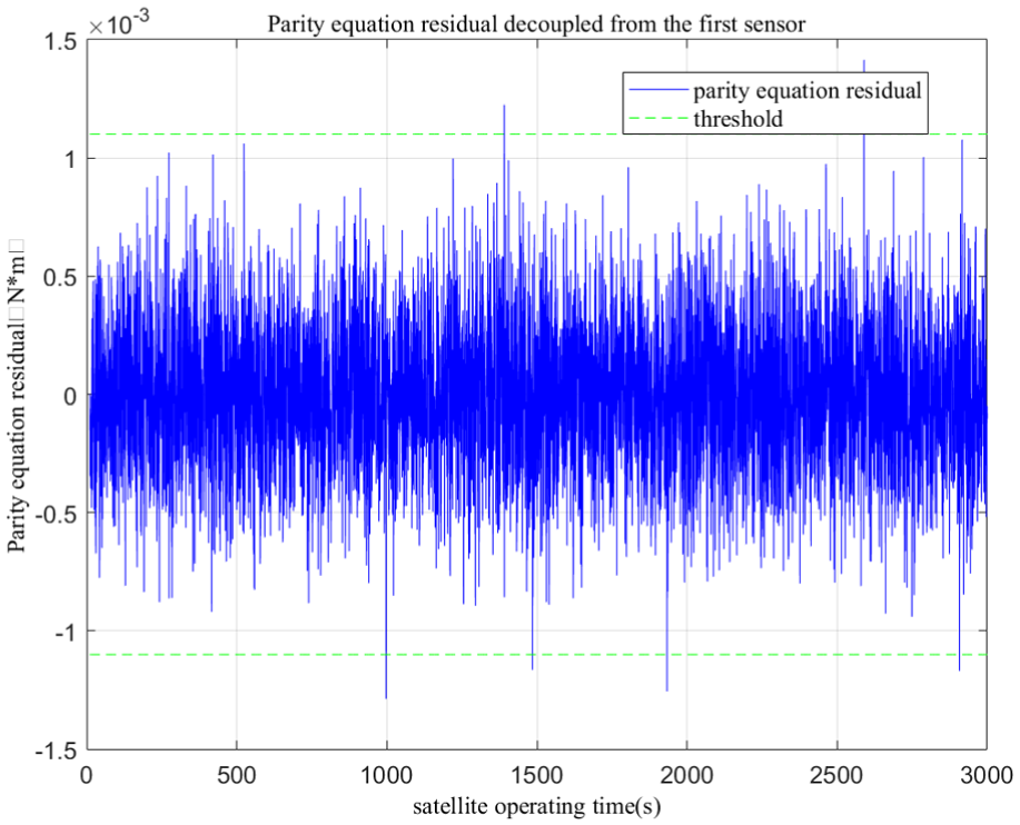
Residual decoupled from the first sensor.

Figure 10.

Residual decoupled from the second sensor.

The aforementioned method is used to detect and isolate a sensor fault under the single fault condition. Because the measurements of different sensors and the projections of the measurement results in different FDPV directions are different, the residual form of the parity equation may be different.

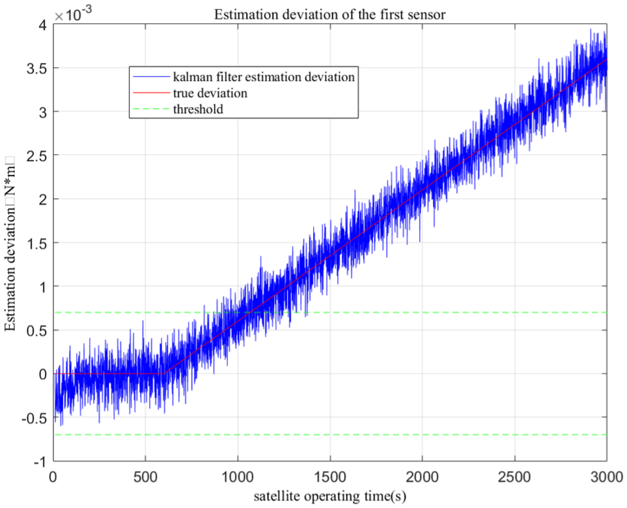
After fault detection and isolation, the fault parameters are estimated using equations (54) and (58). The simulation results are shown below.

Figure 11 shows that estimation of the fault parameter can be achieved by designing a reduced-dimension FDPV. Some errors exist in the estimation results before or after the time at which the fault is added, and there is a jump in the residual of the parity equation. The fault parameters can be estimated accurately during the remaining period.

Figure 11.

Estimation results for an abrupt fault at the first sensor.

A time-varying fault at the first sensor is expressed as equation (60). The simulation results are shown below

$${\beta }_{\mathrm{si}}=\{\begin{array}{cc}0\hfill & \hfill t<600\mathrm{s}\hfill \\ \multicolumn{1}{c}{1.5\times {10}^{-6}\times (t-600)}& \hfill t\ge 600\mathrm{s}\hfill \end{array}$$

(61)

Figures 12 and 13 show that this method can also be used to detect and isolate time-varying faults. When the first sensor is faulty, the residual decoupled from the first sensor is a white-noise sequence. The parity residual that is decoupled from the second normal sensor goes awry because it is affected by the fault.

Figure 12.

Residual decoupled from the first sensor.

Figure 13.

Residual decoupled from the second sensor.

The estimation results for a time-varying fault are shown in Figure 14.

Figure 14.

Estimation results for a time-varying fault at the first sensor.

Figure 14 shows that based on the fault isolation, the reduced dimension of the FDPV can be used to estimate the parameter of a time-varying fault.

To verify the fault diagnosis of the decoupled FDPV for multiple sensors, the results for the case in which a fault is added at the first sensor are shown in equation (60); those for the case in which a fault is added at the third sensor are shown in equation (61). The simulation results are shown in Figures 15 and 16.

Figure 15.

Decoupling vectors for the first and third sensors.

Figure 16.

Decoupling vectors for the second and fourth sensors.

Figures 15 and 16 show that when multiple sensors are faulty, the parity residual result of the zero-mean white noise can be obtained only by designing the FDPV for two faulty sensors; otherwise, the fault information will be reflected in the residual. Thus, fault diagnosis and isolation of multiple sensors are achieved. In addition, the projection in the direction of the FDPV is different for different sensor faults. The residual shown in Figure 16 indicates that the projection in the direction of the residual of the abrupt sensor fault is more obvious.

Conclusion

This article introduces a fault diagnosis method for the actuators and sensors in a closed-loop control system. Closed-loop control system equations and fault modes are presented. An actuator fault can affect both the system measurement output and system state. The fault will be propagated with the feedback loop, which will affect the system input and the system state equation. Sensor faults affect the system measurement output while disturbing the actuator input, which impacts fault isolation.

The residual generated by the FPE is sensitive only to a specific actuator and is decoupled from the system state and other actuators. The residual is obtained by establishing the FPE for each actuator, and then the fault model parameters can be estimated. In this manner, the fault detection and isolation of actuators in a closed-loop system are achieved. A double parity equation diagnosis method for sensor faults in a closed-loop system is used to detect and isolate sensor faults and to achieve fault parameter estimation that allows the single and multiple fault diagnosis isolation of sensors in a closed-loop nonlinear system.