
Abstract
It is a great challenge to offer a fine-grained and accurate PM2.5 monitoring service in urban areas as required facilities are very expensive and huge. Since PM2.5 has a significant scattering effect on visible light, large-scale user-contributed image data collected by the mobile crowdsensing bring a new opportunity for understanding the urban PM2.5. In this article, we propose a fine-grained PM2.5 estimation method based on random forest with data announced by meteorological departments and collected from smartphone users without any PM2.5 measurement devices. We design and implement a platform to collect data in the real world including the image provided by users. By combining online learning and offline learning, the method based on random forest performs well in terms of time complexity and accuracy. We compare our method with two kinds of baselines: subsets of the whole data sets and six classical models (such as logistic, naive Bayes). Six kinds of evaluation indexes (precision, recall, true-positive rate, false-positive rate, F-measure, and receiver operating characteristic curve area) are used in the evaluation. The experimental results show that our method achieves high accuracy (precision: 0.875, recall: 0.872) on PM2.5 estimation, which outperforms the other methods.
Keywords
Introduction
Since atmospheric pollutants may cause respiratory diseases such as lung cancer and severe environmental problems (NASA climate research, http://climate.nasa.gov/causes/), urban air pollution is a critical issue in both developed and developing countries. It is necessary to give relatively accurate evaluation and analysis of air pollution in urban areas.
To communicate to the public the levels of the air pollution, such as the concentrations of
Previous studies on air pollution monitoring are mainly based on wireless sensor networks (WSNs) and Internet of Things.
1
In static sensor networks (SSNs), sensors are usually placed on walls or street lamps. For example, CitySense
2
aims to provide an urban-scale wireless networking testbed for air pollution monitoring. In vehicle sensor networks (VSNs), sensor nodes are usually deployed on buses or taxis. For example, Völgyesi et al.
3
present the mobile air quality monitoring network system by a large number of car-mounted sensor nodes. As gas sensors are usually of low cost, lightweight, and with a fast response time, the programs above have a good performance on gas pollution monitoring. However, to monitor the
In recent years, the large-scale user-contributed data provided by participatory sensing6–8 bring a new opportunity for understanding the air pollution in the city. Photos shared by users are valuable resources. According to the principle of Mie scattering,
9
To achieve the fusion between irregular real-time data (the photos collected by spontaneous volunteers and motivated participants) and fixed data (the official data published by relevant agencies), two main problems need to be solved: (1) correlation analysis of data and (2) modeling and inference for heterogeneous data.
The correlation analysis of
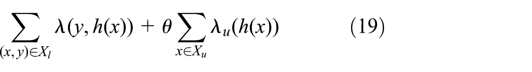
To make the best use of the heterogeneous data, the MCS-RF model combined with offline learning and online improvement has been proposed in this article. We apply the MCS-RF model to infer the real-time and fine-grained
Related work
There is a lot of research on air quality monitoring based on WSN in the past few years. At present, there are three ways to achieve the air quality monitoring: SSN, VSN, and community sensor network (CSN). In SSN, the sensor nodes are typically mounted on the streetlight or traffic light poles or walls.2,14 It can provide accurate and reliable data and can also guarantee the network connectivity. However, to achieve the fine-grained air quality monitoring, many sensors and a customized wireless network are required. What is more, the SSN may also cause resource waste
15
In VSN, the sensor nodes are typically carried by the public transportations like buses or taxis
3
With the development of the vehicular networks,
16
the VSN can provide accurate and reliable data, and the sensor nodes have high mobility. However, to achieve fine-grained air quality monitoring, the cost inefficiency on carriers could be very high. Uncontrolled or semi-controlled mobility cannot be accepted in this way. Also, the spatial-to-temporal resolution trade-off problem cannot be ignored.
17
In CSN, the sensor nodes are carried by the public or professional users.
18
Since the sensors used are usually very cheap and easy to operate with low accuracy, the quality and quantity of the data can be very poor in some situation. For
There have been many studies on estimating the extinction coefficient and the transmittance of the scene based on the photos. He et al.
12
use the dark channel to remove the haze by calculating the transmittance with a single photo. Graves and Newsam
19
use the spatial contrast to estimate atmospheric light extinction with cameras. As the wavelength range of visible light in air is between 390 and 780 nm, according to Mie scattering principle,
20
the fine particulate matter with the diameter in the range of 0.38–0.78 (the major component of
The mobile crowdsensing and computing (MCSC) and Internet of Things have been developing fast in recent years. 21 The MCSC applications mainly focus on environment monitoring, transportation, traffic planning, and urban dynamics sensing with smartphones. Maisonneuve et al. 22 measure and map noise pollution with mobile smartphones’ microphone. Eisenman et al. 23 deploy BikeNet, an extensible mobile sensing system to measure the air pollution. Cui et al. 24 schedule tasks fairly for large-scale mobile device systems with mobile cloudlets. Yang et al. 25 propose an incentive mechanism design for mobile phone sensing. F Restuccia and SK Das 26 propose a trust-based framework for secure user incentivization in participatory sensing. Xiao et al. 27 apply a deep Q-network (DQN) to derive the optimal MCS policy against faked sensing attacks. With the rapid development of video technology, the hybrid unicast/multicast adaptive videos 28 may also be used for environment prediction in the future.
Framework of the MCS-RF
MCS-RF is made up of five parts as shown in Figure 1: Data Collection, Data Storage, Model Training, Inference, and User Interaction.
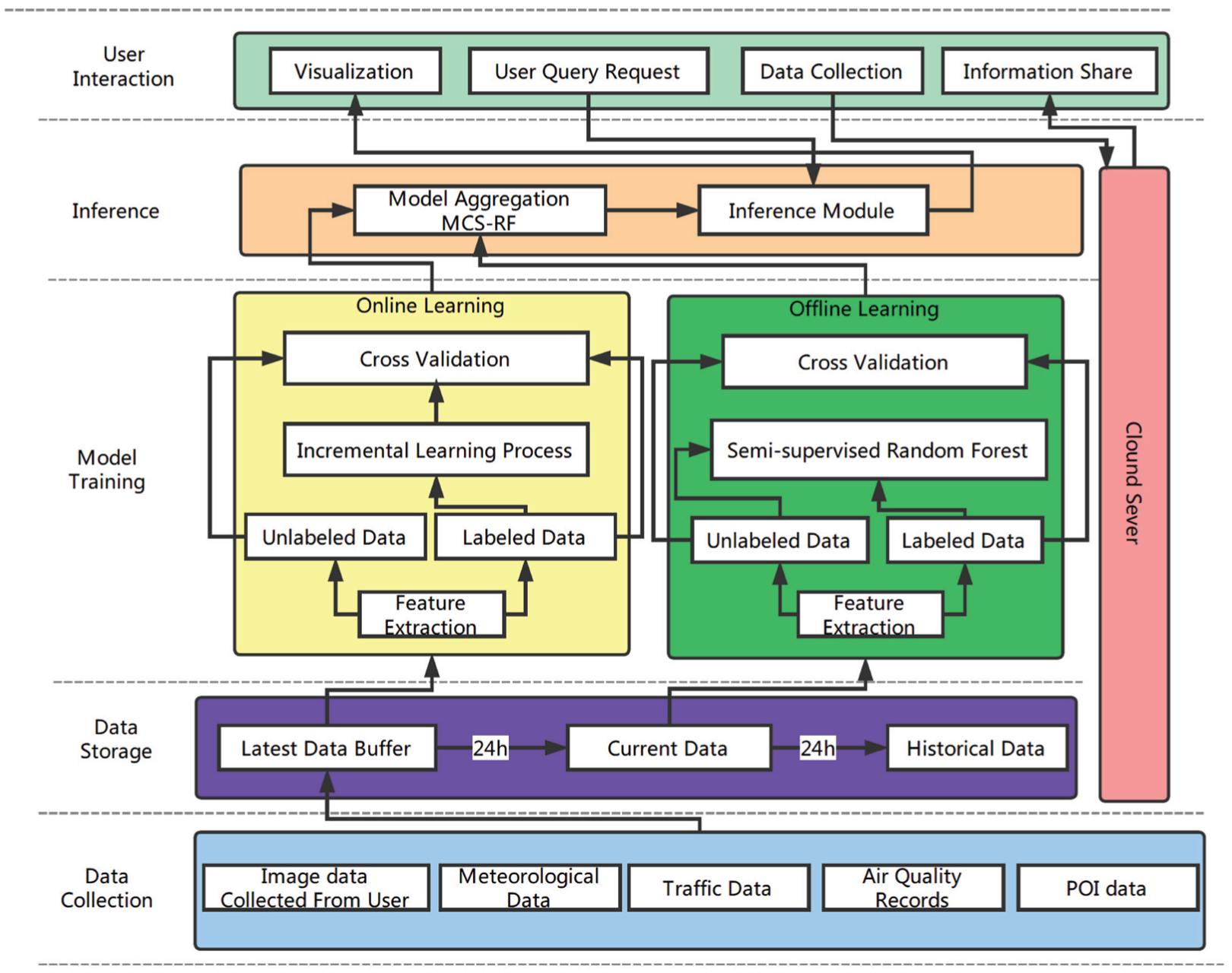
The framework of the MCS-RF.
Data Collection
Data Collection is responsible for collecting raw data. The data collected are made up of two major parts: the user-contributed image data collected by smartphones and the public data published by relevant functional departments. In recent years, smartphones have been very popularized in cities and photography is one of the basic functions of smartphones; compared with the other methods based on additional equipment, our method can easily attract more participants. The user clients only upload their photos with the time stamp and GPS information, the cloud server receives the photos and collects other data from the public websites, usually published by the government.
Data Storage
Data Storage is made up of three parts: Latest Data Buffer module is used to store the data updated in real time and send the data to the Online Learning module, the Current Data module updates every 24 h which receives the new data from the Latest Data Buffer module and sends its data to the Offline Learning module and the Historical Data module; the Historical Data module only takes responsibility for the data storage.
Model Training
Model Training consists of two parts: offline learning and online learning. Offline learning achieves the initialization of the forest with all data sets every 24 h. An SRF method is applied to offline learning. Online learning achieves the adaptive incremental learning based on the data arrived in real time.
Inference
Inference takes responsibility for the major function of the platform. It stores the inference model based on the models provided by online learning and offline learning. When the user requests arrive, Inference calculates the final evaluation value based on the data collected from the user and returns the results to the User Interaction module.
User Interaction
User Interaction is applied on the users’ smartphones, which makes contributions to the user experience and also uploads the image data collected by the users.
Problem statement
This paragraph presents the problem definition and notations. Given a collection of grids
Correlation analysis between PM2.5and image
According to the principle of Mie scattering,
9
Image preprocessing
Our image analysis method is based on mobile phone cameras, and most mobile phones contain image processing functions which often apply non-linear transformation that maps the observed image from the irradiance to the brightness. We use the radiometric calibration method to recover the image. 29
Mobile phone photos usually contain two parts: the sky and the scene. These two parts are quite different in image features. S Poduri et al. 30 use sky luminance to estimate air turbidity with mobile phones. It is very necessary to separate the sky area and the scene area with a low-complexity algorithm. We find that, in most of the images of outdoor scenes, if we divide the image into nine parts (3 × 3), there will always be some parts which have little sky or scenery. We collect photos taken by mobile phones from different locations in Beijing and divide each image into nine parts. By calculating the image features of different parts, we find that, if the images are converted from RGB model to HSI model, there would be a significant difference in the variance of intensity between the sky part and the scene part. According to the above conclusions, when we get a new image to estimate PM2.5, it would be divided into nine parts. By calculating the variance of intensity of each part, we choose the highest three parts as the SCPs (scenery parts), which will be used in the extraction of dark channel features and the lowest part as the SKP (sky part), which will be used in the extraction of HSI color features.
Spatial contrast (Fig)
Atmospheric transmission refers to how well light radiating from a scene is preserved when it reaches an observer. The atmospheric transmission model

has been widely accepted nowadays, where

where

transmission has the intuitive interpretation as the ratio of the observed contrast to the true contrast. So we define
Dark channel (Fid)
The dark channel feature, recently proposed by He et al., 12 has been widely used in haze removal. Based on the assumption that there is at least one color channel including pixels with very low or close-to-zero intensity in most of the non-sky blocks of the image. In this situation, only the SCPs will be used in this situation. The dark channel of an image is defined by
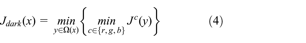
where

By applying dark channel prior to equation (1), the estimated transmission

where

where
HSI color difference (Fih, Fis, Fii)
According to Kim and Kim’s
32
study, the sky’s color difference in the HSI color space has an exponential relation with the light extinction coefficient

where a and b are the coefficients in this model and
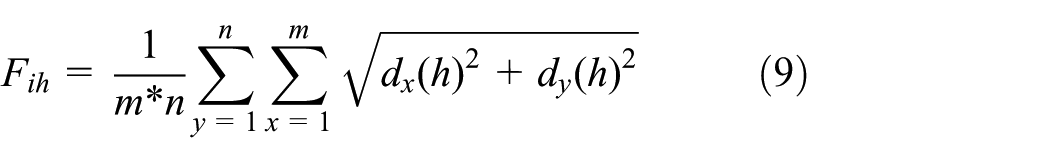


where I is the input image with


Correlation analysis
Figure 2 shows the correlation matrix between the image features
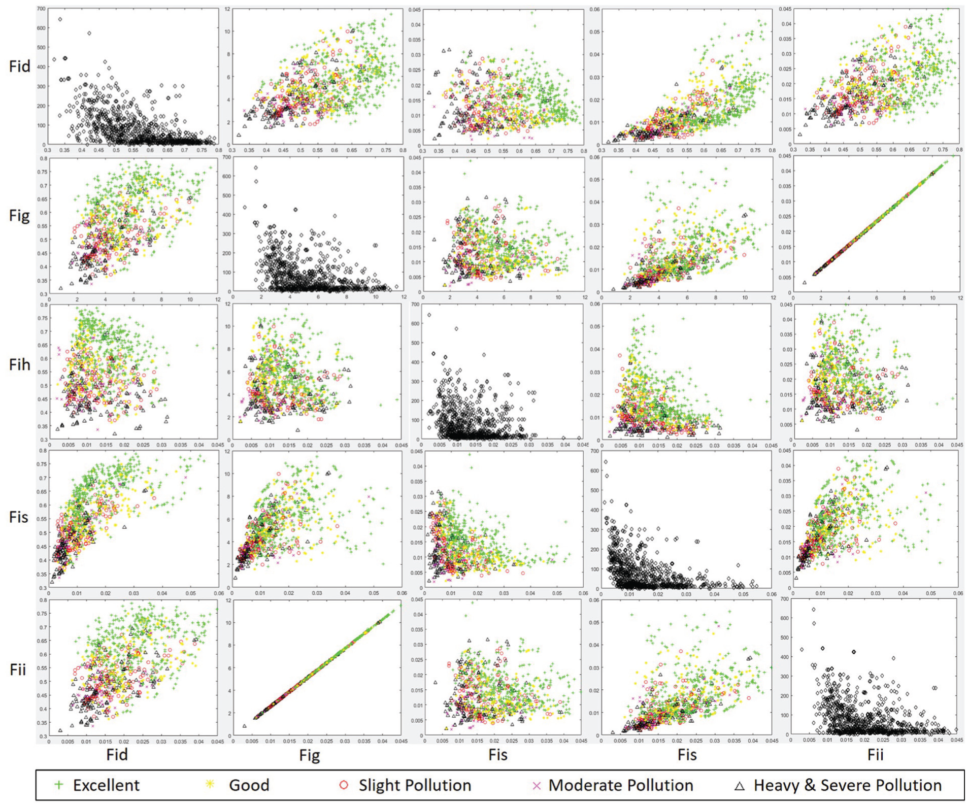
Correlation matrix between Fi and
MCS-RF: a random forest–based approach
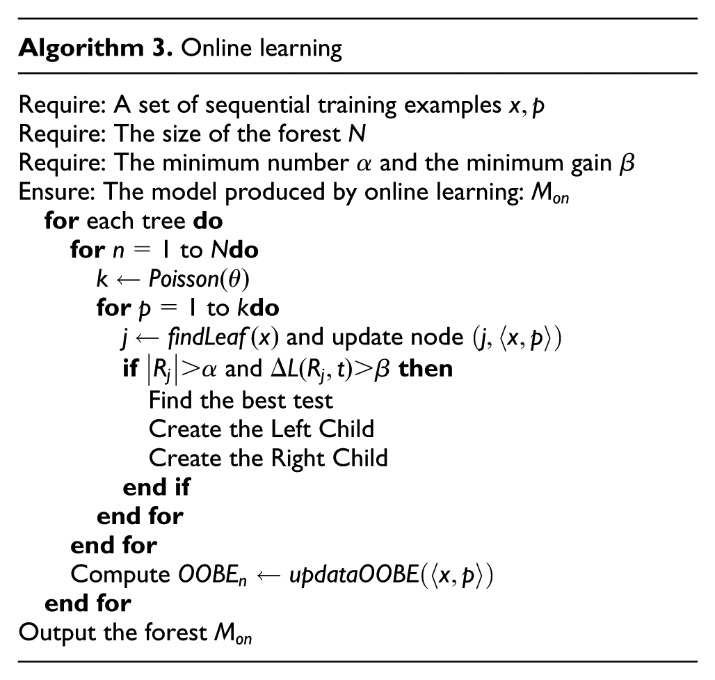
The MCS-RF is divided into two parts: offline learning and online learning. Since there are only a few air quality monitoring stations, most data are unlabeled, and we use the SRF 33 model to perform the offline learning process. As the image data in our system are collected in real time, to improve the estimation accuracy, the ORF 34 model is used to achieve the incremental learning. The two models are combined in our system as shown in Algorithm 1.

Random forest
A random forest (RF) is a set of decision trees. Each tree in the forest is built and tested independently from the other trees.
We denote the

where

In this article, we define the classification margin of a labeled sample

and from equation (16) we can easily obtain the conclusion that, if the classification is correct,

where E is the expectation which can be measured by the the entire distribution of

In this equation,
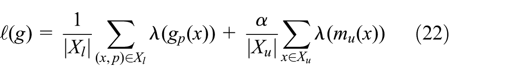
Offline learning
For many semi-supervised learning algorithms, the supervised loss function of unlabeled instances can be defined in the form of
where
Since we target applications with a large amount of data and manifold regularization leads to algorithms that are quadratic, that is,

The margin for the unlabeled data is defined as

Based on the definition of the margin for unlabeled samples, the overall loss can be defined as
where
In semi-supervised learning, we directly monitor the strength of the ensemble by measuring the out-of-bag estimation (OOBE), which has been proved to be a good estimate of the generalization error.
39
The detailed algorithm is shown in Algorithm 2. The time complexity has been proved by Leistner et al.
33
that the SRF in this way is quite similar to the supervised random forest, which usually has a time complexity of

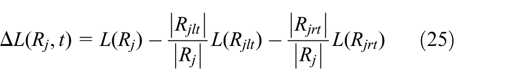
Online learning
To perform online bagging, we use N Oza and S Russell’s
40
method where the sequential arrival of the data is modeled by a Poisson distribution. That means for each tree

or the Gini index

where
where
Evaluation
This section consists of three parts: the first part introduces the basic structure of the experiment; the second part offers the basic description of contrast algorithms; and the third part shows the results and the analysis.
Preliminaries
In this subsection, the standard of classification, data origin, evaluation index, and the ground truth will be fully discussed.
Concentration levels of PM2.5
AQI is a number used by government agencies to communicate to the public how polluted the air is currently. Different countries have different definitions of AQI. In China, the AQI is based on the levels of six atmospheric gasses, namely,

The definition of AQI in China.
Datasets
In the experiments, the data were collected from May 2014 to March 2015, and the following datasets of Beijing are all available to the public except the image data. Most of the data are unlabeled except those collected from the air quality monitoring stations.
Mobile crowdsensing data
Data collected by mobile crowdsensing have the characteristics of flexibility on temporal and spatial distribution. The data collector can obtain data from specific areas easily with the incentive mechanism. However, it is hard to guarantee the quality of the mobile crowdsensing data and the irregular real-time data can also bring challenges to data fusion. In this article, the mobile crowdsensing data consist of image data.
Image data. The image data consist of photos taken by the participants with their smartphones, from May 2014 to March 2015 in Beijing. All the photos uploaded to our participatory sensing platform have accurate GPS information. The photos near the
Generic data
Generic data in this article consist of meteorological data, traffic data, POI data, and air quality monitoring station data. The data in this dataset have fixed spatial distributions and update regularly. Especially, the data with high accuracy collected from the air quality monitoring stations make up the labeled datasets.
Meteorological data. Accordingly, we collect the meteorological data from the government website (Meteorological data, http://data.cma.cn/) and identify five features: humidity (Fwh), temperature (Fwt), wind speed (Fws), barometer pressure (Fwb), and weather (Fww). The weather features are classified into five categories: sunny, cloudy, foggy, rainy, and snowy.
Traffic data. We employ traffic features based on grids from Baidu maps. The pixels of different colors (green, yellow, red) can describe the traffic condition. We collect the fine-grained traffic status (green, yellow, and red) from the website (Baidu map, http://map.baidu.com/) and calculate the traffic features for each grid every hour.
Air quality records. We collect real-valued AQI of six kinds of air pollutants, consisting of
POI. We employ a POI database from Baidu maps to extract
Combined Data
Combined data are the combination of the mobile crowdsensing data and the generic data.
Grid
We divide the city into disjointed grids (e.g. 1 km × 1 km) and assume that the air quality in a grid is unified. Each grid g has a geographical position coordinate
Evaluation index
The evaluation indexes we used in this article are shown in Table 1.
Evaluation index.

TP: true positive; FP: false positive; ROC: receiver operating characteristic.
Ground truth
We deliberately remove a station from a grid and infer its PM2.5 from the other stations. The actual
Baselines
We compare our method with six baselines and the ratio of the datasets for cross-validation is 10%.
Logistic
It is a classification model for building and using a logistic regression model with a ridge estimator.
Naive Bayes
It is a classification model for a naive Bayes classifier using estimator classes. 41
Random tree
It is a classification model for constructing a tree that considers K randomly chosen attributes at each node. We perform no pruning in the experiment.
Back-propagation neural network
Back-propagation neural network (BP ANN) is a classifier that uses back-propagation to classify instances, which is used by U-Air. 4
Sequential minimal optimization
Support vector machine using sequential minimal optimization (SMO) is a classifier which replaces all missing values and transforms nominal attributes into the binary ones. 42 This method is widely used in classification problems in recent years, such as the classification of smartphones apps. 43
K*
K* is an instance-based classifier, is the class of a test instance based on the class of those training instances similar to it, and uses an entropy-based distance function. 44
Results
In this subsection, the overall results are discussed first, which have proved that MCS-RF performs best on the overall average index. Second, the results of classifications are fully discussed, which have proved that MCS-RF has obvious advantages on the indiscernible classifications such as slight pollution and moderate pollution. Finally, the results of features have proved that the image features have obvious promotions on most of the classifications, especially for the indiscernible classifications.
Results of features on the whole
In this area, Zheng et al.
4
have already proved that the meteorological data, traffic data, POI, and the air quality records have a close relationship with the air quality. As shown in Figure 2, the image features have a fuzzy relationship with
Results of features on the whole for all models.
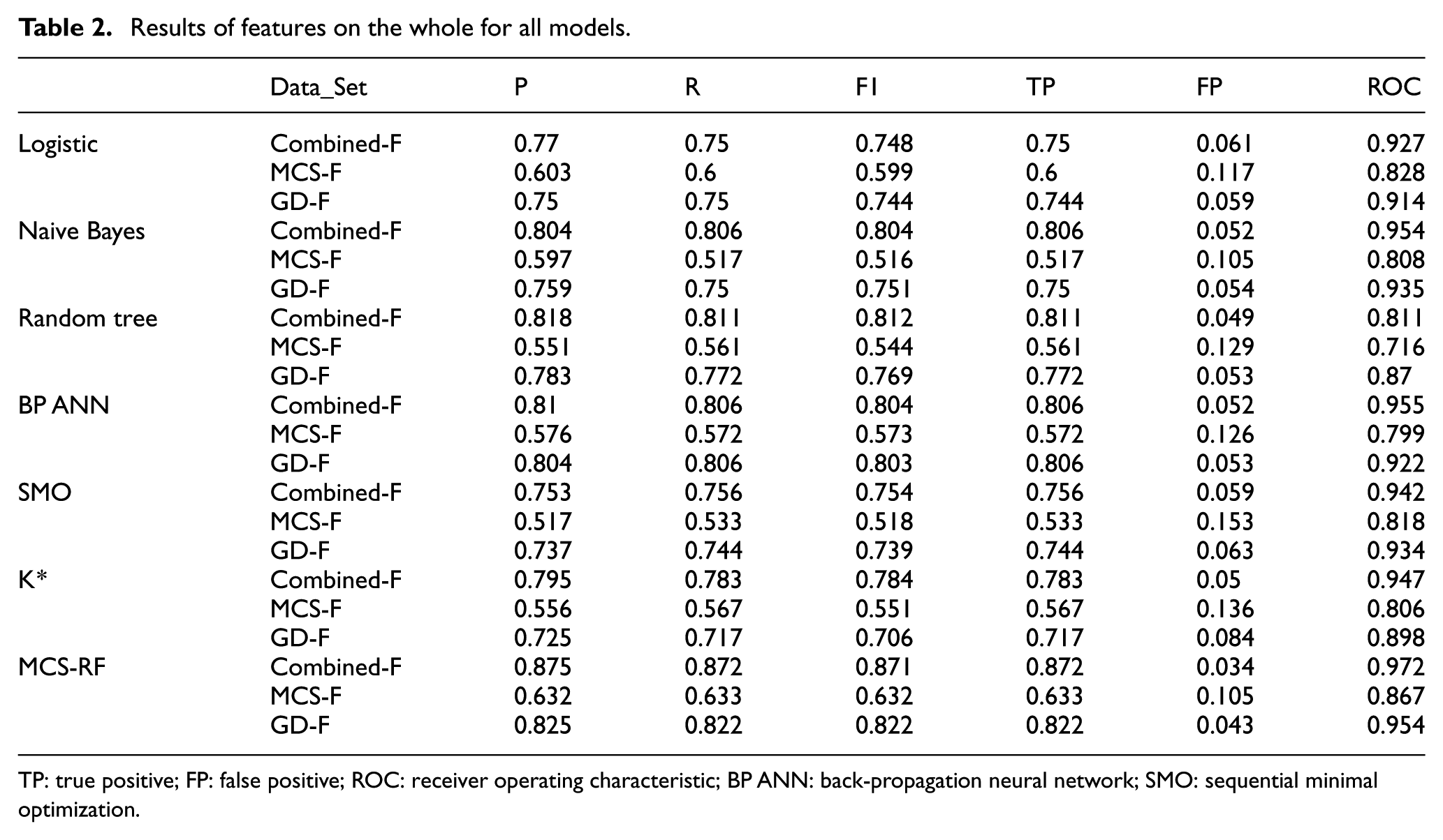
TP: true positive; FP: false positive; ROC: receiver operating characteristic; BP ANN: back-propagation neural network; SMO: sequential minimal optimization.
On the other hand, the results also demonstrate the advantage of our method over logistic, naive Bayes, SMO, K*, and random tree models based on our data sets in this situation.
Results of the classifications of all models
The evaluation of the overall index is not enough. As shown in Figure 4, the precise classification into good, slight pollution, and moderate pollution can be hard in this situation, while the classification into excellent and heavy & severe pollution can be much easy. In daily life, if the air pollution level has exceeded moderate pollution, outdoor activities are not advised. On the other hand, if the air pollution level is good, even if the the weather looks bad, it makes no sense on outdoor activities. Figure 4 shows the results of precision, and different models have quite different performance on the classifications. Our method has great improvements on the classifications of good, slight pollution, and moderate pollution, while our method has the same performance on the classifications of excellent and heavy & severe pollution. Finally, our method has a significant improvement on average. Figure 5 shows the results of recall, and the conclusion is almost the same except on the classification of heavy & severe pollution; our method is slightly worse than naive Bayes. Figures 6–9 show the results of other indexes, and our method has obvious advantages in this situation.

Precision of the classifications.

Recall of the classifications.
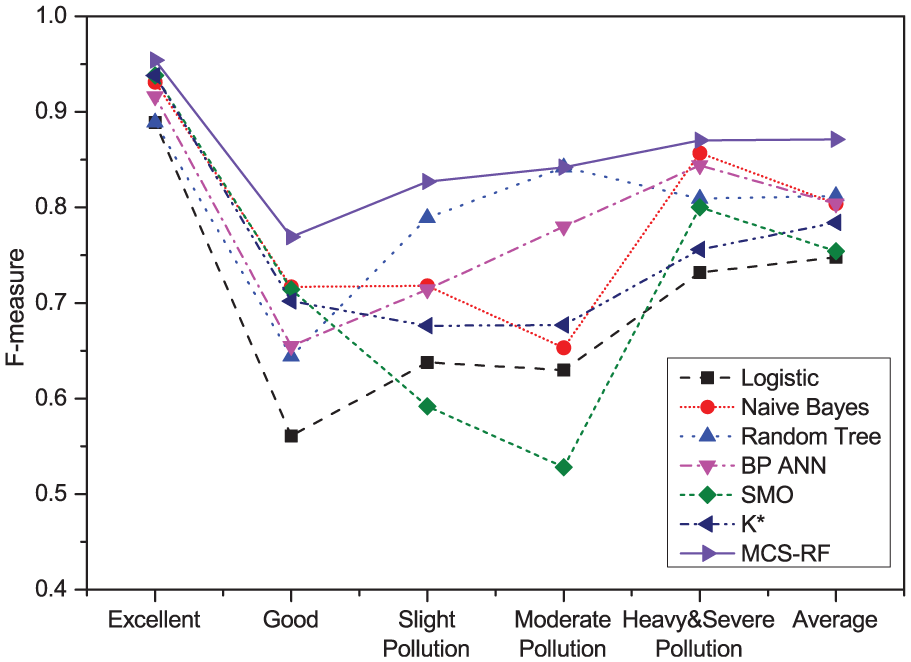
F-measure of the classifications.

TP rate of the classifications.

FP rate of the classifications.

ROC of the classifications.
Results of the features on classifications of MCS-RF
Figure 10 shows the classification results of precision based on MCS-RF. Although the image data have poor performance on the air quality estimation, when we add the image feature sets into the model, it can always bring a significant precision improvement on all classifications. Especially, the image features have a good performance on the classification of the moderate pollution, and the overall precision of moderate pollution experiences a sharp increase when we add the image features. The combination of multiple data sources could be very necessary when the problem we faced is very complex. The situation could be very similar when it comes to other indexes. As shown in Figure 11, although the classification of good gets slightly worse, the classification of moderate pollution has almost increased by 51%. When it comes to other indexes such as F-measure shown in Figure 12, the true-positive (TP) rate shown in Figure 13, the false-positive (FP) rate shown in Figure 14, and the ROC area shown in Figure 15, the classifications of slight pollution, moderate pollution, and heavy & severe pollution experience an impressive increase by all.

Precision of the MCS-RF.

Recall of the MCS-RF.

F-measure of the MCS-RF.

TP rate of the MCS-RF.

FP rate of the MCS-RF.

ROC of the MCS-RF.
Conclusion and future work
In this article, we find that several image features are very discriminative in
In the future, to offer a better fine-grained air pollution monitoring service, it is essential to design the incentive mechanism to obtain the image data of some specific areas. Since the image features have strong effects on the evaluation results, the low-quality photos must be removed from our datasets. An algorithm based on image recognition needs to be performed on our cloud servers to achieve the image filtering. The mechanism for user incentive and deception recognition is also needed, and new algorithms can be applied in the future.
Footnotes
Acknowledgements
This paper is an enhanced version of the paper previously published in conference proceedings of 2017 IEEE International Symposium on A World of Wireless, Mobile and Multimedia Networks (WoWMoM’17) entitled “Estimate air quality based on mobile crowdsensing and big data.”
Handling Editor: Daming Zhou
Declaration of conflicting interests
The author(s) declared no potential conflicts of interest with respect to the research, authorship, and/or publication of this article.
Funding
The author(s) disclosed receipt of the following financial support for the research, authorship, and/or publication of this article: This work was partly supported by the National Natural Science Foundation of China (Nos 61370197, 61402045, and 61602051), Research and Technology Verification of Address-Driven Network Architecture (2015 AA015601), and Research on Architecture and Key Technology System of Service-Oriented Software-Defined Network (2015AA016101).