Sage Journals: Discover world-class research

Abstract

A new type of plane strain apparatus is developed to study the mechanical properties and shear band failure of soil, which possesses the advantages of flexible loading for lateral confining pressure and noncontact measurement and high measurement accuracy for surface deformation. In addition, the whole deformation procedure of the specimen can be recorded with images, which can be used to describe the development of strain localization and the shear band. It can be seen that the deformation process has three obvious stages, that is, the hardening stage, the softening stage, and the residual stage. The measured inclination angles of shear bands decrease as confining pressure or the mean size increases. In addition, it can be observed that the sand presents continuing growth of the unrecoverable plastic deformation inside the shear band and exhibits almost elastic deformation outside. From the detection results for local points in the specimen, the stress–strain relationships are different for different parts, and the sand sample behaves like an uneven structure instead of an even element, which means that the usual method of measuring the stress–strain relationship of the soil sample is only a macroscopic approximation.

Keywords

Flexible loading noncontact measurement local deformation measurement strain localization shear band stress–strain relationship plane strain test

Introduction

The phenomena of progressive failure feature of localized shear bands have attracted considerable attention in practical engineering, such as the slope sliding and the foundation instability in the geotechnical engineering. As the shear band failure is easy to trigger and to observe in plane strain state, the plane strain apparatus is developed to serve for the study of the mechanism of the shear band failure in laboratory. Early examples of plane strain apparatuses (such as those developed by Hambly¹) are composed of three mutually parallel rigid plates. The problem of intersection between plates (edge effect) is difficult to be overcome for this type of plane strain apparatus. Finn et al.² developed the Bishop–Cornforth plane strain apparatus with a strip sample (41 cm×5 cm × 10 cm (length × width × height)). To meet the condition $ε_{2} = 0$ , the length in the direction of $σ_{2}$ would be increased, which significantly led to the increase in friction.

The early plane strain apparatus was used only for experiments on the solid particles, and the load and displacement of the specimen can be measured only as a whole. A typical shear band can be identified only when its evolution penetrates the sample. It is difficult to capture the process of localization in detail. Since the 1960s, researchers had developed some complex technologies,^3–15 including the use of transparent confining plates, and internal measurement technology such as X-ray tomography technique for capturing local deformation, and the further development of technologies applied to saturated and unsaturated soils. Also, the ring shear test, which imposes a plane strain boundary condition, is developed to study the shear band formation.¹⁶

The capture of progressive failure and shear band in the soil is a challenge. Despite the challenge, various experimental research works and exploration have been undertaken. The techniques for the measurement of local displacement and strain are developed in these research works. Based on comparisons of stereo photogrammetric and internal linear variable differential transducer (LVDT) data,¹⁷ the displacements were observed at the ends and central portions of the specimen. Once the displacement field has been obtained, various measures of strain can be calculated throughout the specimen, and thus the macroscopic shape of the shear band can also be depicted.

Although LVDT measurement is a very useful instrument in laboratory testing and has high resolution, it is a contact measurement. It may not be suitable for the measurement of deformation at the local points in the specimen. By embedding markers, painting grid points on the sample membrane, the researchers realized the local displacement measurements.^17–19

The computed tomography (CT) technique is particularly effective at detecting the density variations of sand material inside and outside a shear band, so that the shear band patterning, inclination, and thickness may be precisely quantified. Nevertheless, owing to the requirement of radiation sources for this technique, the test can be done only under vacuum confinement at present and the cost may be high, which restricts the precise measurement of the specimen, so the location and thickness of the shear band are merely inferred from variations in microstructure or density data.^20–24

To obtain access to changes in the shear band, we should observe and calculate the strain of the local point from a microscopic view, combining the macroscopic study with the microscopic study. The image-based deformation methods, such as particle image velocimetry (PIV) and digital image correlation (DIC) for the measurement of displacements, velocities, accelerations, and strain fields in geotechnical materials are developed. DIC, as an optical metrology approach first developed by Peters and Ranson,²⁵ has been widely accepted for performing surface deformation measurements. It was developed to quantify local strain on the surface of the specimen, by comparing the digital images of a test object surface acquired before and after deformation.²⁶ It enables quantitative, nondestructive capture of the mesoscale kinematics associated with shear band formation and has been testified that DIC can reliably discern local displacements to an accuracy of at least 0.008 mm.^24,27–31 DIC combined with CT, not only can measure the displacement and strain on the surface of the sample but also can obtain the complex three-dimensional microstructure information, such as strain field, void ratio, and the movements of particles, thus it can also be called the volumetric DIC technique.³²

Recently, the State Key Laboratory of Structural Analysis for Industrial Equipment in Dalian University of Technology has been devoted to the development of the digital image technique to surface deformation measurement in the triaxial tests.³³ Now, the digital image technique is extended to develop a new type of plane strain apparatus. Compared with the LVDT measurement, there are a number of advantages of the new plane strain apparatus: large deformation and noncontact measurement, and the ability to obtain the strains for every point on the surface of the specimen, which has important significance in the analysis of the development of strain localization and formation of shear bands. In addition, the whole deformation procedure of the specimen can be recorded with pictures, which makes it convenient to analyze the state of the specimen at any moment in the experiment.

The new type of plane strain apparatus is introduced in this article. It has two typical characters, that is, flexible loading for lateral confining pressure and the digital image technique for surface deformation measurement. The flexible loading in lateral direction guarantees the uniform distribution of the confining pressure. Based on the digital images technique, which is equivalent to the installation of many sensors in different parts of the sample, the local strain is calculated using the finite element method (FEM) by comparing the digital images of the specimen surface acquired before and after deformation during the plane strain test. Then, the properties of mechanics and deformation of sand under plane strain compression are studied, and a detailed analysis of the strength and deformation of the sand under the plane strain condition is presented. Especially, the capabilities of noncontact and local deformation measurement are exploited to achieve the analysis of the gradual evolution of the shear band and stress–strain relation for local points, and some new findings are given.

The new type of plane strain testing apparatus

Components of the plane strain apparatus

The main components of the new plane strain apparatus include the computer control system, the pressure cell, loading system, digital image measurement system, and related auxiliary equipment. The plane strain apparatus is shown in Figure 1, and its characteristics are as follows:

The axial stress $σ_{a}$ (in the top-down direction) is controlled by the computer program, which can adjust the loading speed. The lateral stress $σ_{c}$ (in the left–right direction) is controlled by two flexible membranes, into which the pressure water can be injected to maintain a stable confining pressure.

The condition $ε_{b} = 0$ is ensured using a fixed rear baffle and a fixed front baffle, which are made of tempered glass. Images are captured via the digital image measurement system. The deformation of the specimen and the strain distribution are processed by computer image processing software.

The plane strain apparatus is easy to operate. It requires only that the operator makes the sample and input parameters. The testing work is completed automatically by the controlling system.

Figure 1.

The plane strain apparatus.

The pressure cell

The pressure cell is shown in Figure 2. The main components of the pressure cell include the bottom plate, lateral membrane components, rear baffle, pressure bar, and front window made of the transparent tempered glass. The bottom plate is located at the bottom of the pressure cell, connecting the computer and the pressure cell. The lateral baffles connecting membrane, together with the rear baffle tightened by screws, make up the inner cavity of the pressure cell. The transparent tempered glass together with rear baffle makes $ε_{b} = 0$ , and the tempered glass facilitates clearer photographs also. The size of the sample is 100 mm (height) × 60 mm (width) × 100 mm (thickness). The pressure cell is fixed on the rear baffle to prevent it from moving downward.

Figure 2.

Pressure cell.

The loading system

The loading system of the plane strain apparatus mainly consists of two parts: one part is the load of the vertical stress $σ_{a}$ , which is controlled by the load sensor, and the other is the load of the lateral confining pressure $σ_{c}$ . $σ_{a}$ is given by the load sensor and imposed by the movement of the loading cap assembly on the beam when it touches the pressure cell. The capacity of the load sensor is 10 kN with resolution of 25 N. The inner cavity of the pressure cell includes the lateral baffles, rear, and front baffles made of toughened glass. $σ_{c}$ is applied by water pressure in the membrane, which is generated by water pressure generator and controlled by the water pressure sensor with capacity of 1.0 MPa and resolution of 2.5 kPa. The membrane full of water is shown in Figure 3.

Figure 3.

The membrane full of water.

The measurement system

The image measurement system consists of the complementary metal-semiconductor (CMOS) camera, computer, and image processor software. The technical indexes of the camera are as follows: the resolution 1280 × 1024 pixels, the focal length 16 mm, the lens aberration rate less than 0.1% with the smallest view of 165 mm × 124 mm, and the physical size for each pixel 5.2 µm × 5.2 µm. The images of the entire surface of the specimen, captured by the CMOS camera at the appropriate time interval and saved by computer automatically, are transformed and processed by the computer image processor software.

Figure 4 is an image captured after the installation of the specimen. The specimen is wrapped in a black rubber membrane, on which 32 white squares are drawn to mesh with screen printing technique, and the nodes of the black and white grid on the image (shown in Figure 4) can be recognized using a sub-pixel corner detector algorithm. There are 128 corner nodes for 32 white squares. Tracking these nodes, we can obtain their displacements; then, by taking each black and white square as a four-node element, the strain on the entire surface of the specimen can be calculated. Y Li³⁴ conducted the error correction and data processing of digital image measurement based on plane strain experiment and proved that the calibration outcome is accurate and effective.

Figure 4.

Measured image for the sample.

The strain calculation

During the plane strain test, images of soil specimen can be obtained by the digital image measurement system. These images are recorded by pixel values. Using pixel equivalent transformation, the coordinates of the element nodes on the entire surface of a specimen can be obtained.

Then the strain in each element is calculated using the FEM according to the displacement of the nodes. All the corner points are taken as the nodes of four-node element, and the strains are calculated thereafter.³³ Mapping element and four-node mother element are shown in Figure 5(a) and (b), respectively.

Figure 5.

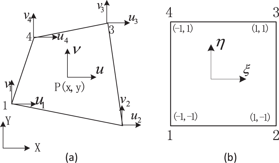
Strain calculation with FEM: (a) mapping element and (b) four-node mother element.

Coordinates of any point on the surface can be obtained by interpolation

{\begin{matrix} x = \sum_{i = 1}^{4} N_{i} X_{i} \\ y = \sum_{i = 1}^{4} N_{i} Y_{i} \end{matrix}

(1)

where $X_{i}$ , $Y_{i}$ are coordinates of element nodes and $N_{i}$ is the shape function. For four-node element, the shape function can be written as follows

N_{i} = \frac{1}{4} (1 + ξ_{i} ξ) (1 + η_{i} η) i = 1, 2, 3, 4

(2)

in which $(ξ_{i}, η_{i})$ are the node coordinates of the mother element.

Set $(X_{i}^{0}, Y_{i}^{0})$ to the initial configuration of the node coordinates, then the displacements $(u_{i}, v_{i})$ of each node can be obtained by

{\begin{matrix} u_{i} = X_{i} - X_{i}^{0} \\ v_{i} = Y_{i} - Y_{i}^{0} \end{matrix}

(3)

For four-node element, the displacements $(u, v)$ of any point on the surface can be written as follows

{\begin{matrix} u = \sum_{i = 1}^{4} N_{i} u_{i} \\ v = \sum_{i = 1}^{4} N_{i} v_{i} \end{matrix}

(4)

Thus, the strains at any point can be given

{ε} = {\begin{matrix} ε_{x} \\ ε_{y} \\ γ_{xy} \end{matrix}} = {\begin{matrix} \frac{\partial u}{\partial x} \\ \frac{\partial v}{\partial y} \\ \frac{\partial u}{\partial y} + \frac{\partial v}{\partial x} \end{matrix}} = [B] {\begin{matrix} u \\ v \end{matrix}}

(5)

where $(ε_{x}, ε_{y}, γ_{xy})$ are horizontal strain, vertical strain, and shear strain, respectively; $B$ is the strain–displacement transformation matrix, which can be obtained according to standard finite element analysis process.

In this way, the deformation distribution over the entire surface of the specimen is obtained by digital image measurements during plane strain test; then, the strain distribution is derived from the measured deformation. Also, the corresponding strain contour map can be drawn by the software (Surfer 8.0 by Golden Software Company).

To confirm the reliability of measurement results, the measurement precision is estimated by comparing the strain from the digital image system with that from the strain gauges.³³ It is given that the difference between the “true values” and the “test values” of the strain is approximately 0.0001, which means that the measurement precision of the plane strain test can be satisfied.

Testing process

The testing process is as follows:

Sample preparation. According to the relative density designed for the test and the maximum and the minimum dry density of the sand, determine the dry density and the corresponding mass for the sand specimen first. Then, get the amount of sand and divide it into three parts averagely and pack them into the barrel evenly in turn to guarantee the same volume for each part after tamping. Finally, carefully trim and smooth the top surface so the specimen to minimize the occurrence of shear band–platen interference.

Sample installation. The specimen is connected with vacuum pipes at the top and bottom parts and evacuated by vacuum machine first, so that the sand sample can stand after the membrane tube is removed. Then, place the sample on the bottom of the pressure cell and fix it.

Installation of the pressure cell. Install the lateral membrane and check for water leakage. To facilitate the installation and prevent the membrane from being sandwiched between the parts, generally keep the membrane dry and vacuum. Then, install and fix the glass window and brush a layer of lubricating oil on the glass to reduce the friction between the glass and the membrane.

Sample saturation. First, supply about 20 kPa water pressure in the membrane, namely, the confining pressure; then, close the switch of the vacuum pump and open the drainage switches connected with the bottom of the pressure cell and the sample cap; next, pour carbon dioxide (CO₂) into the sample by a quick joint for about 20 min; after that close the quick joint and shift to inject air-free water into the sample until the volume of the air-free water flowing through the sample is about three times that of the sample.

Image acquisition preparation. Open the image measurement system and adjust the camera such that it can capture a clear image; then, start to collect the data.

Sample consolidation. Supply water pressure in the membrane, that is, the lateral confining pressure generated by water pressure generator. The saturation degree can be tested by observing the change of pore water pressure with the confining pressure. Open the drainage switches connecting with the membrane to let the water drain out, so the sample can be consolidated.

Start the test. After the consolidation of the sample, open the digital image measuring system and input the required parameters into the control system first. Then, set the shearing speed to 0.2 mm/min. After that, apply the axial load and start the test.

Termination of the test. Stop the test as the axial strain gets to 20%. Then, unload the confining pressure and axial load, turn off the instrument, and so on.

The testing materials

The granular material tested is the Fujian (China) sand. The Fujian sand is a quartz sand, in which the content of silica is more than 96%. Three different mean sizes of sand are used in the experiment. The particle-size distributions of sand are given in Figure 6. The physical properties of these three kinds of sand are given in Table 1. The maximum dry density and the minimum dry density are determined in advance based on the method of measuring cylinder and the method of vibration tapping (Chinese Geotechnical Testing Method and Standard, GB/T 50123-1999), respectively. The dry density can be calculated according to the relative density assigned for the specimen in the experiment and is given in the following parts.

Figure 6.

Particle-size distributions of the sand used in the study.

Table 1.

Physical properties of the tested sand.

Sand number	Mean size $d_{50}$ (mm)	Min. dry density ${ρ_{d}}_{min}$ (g/cm³)	Max. dry density ${ρ_{d}}_{max}$ (g/cm³)	Curvature coefficient $c_{c}$	Uniformity coefficient $c_{u}$
1	0.23	1.33	1.77	1.73	3.33
2	0.75	1.39	1.64	4.28	6.0
3	1.5	1.35	1.60	4.15	6.52

Study on the mechanical properties of sand based on the plane strain test

The relationship between the stress difference and the axial strain

Figure 7 shows the relationship between the stress difference and the axial strain in the plane strain test as D_r = 60%, $d_{50} = 0.23 mm$ , and the confining pressures are 50, 100, and 150 kPa, respectively. It shows that when the strain is small, the stress difference increases with increasing axial strain until the curve reaches its peak value. This stage belongs to the hardening stage. As the test continues, the axial strain increases continuously while the stress difference decreases, which belongs to the softening stage. When the strain is large enough, the stress difference gets to a constant value and a residual stage arrives.

Figure 7.

Relationships between stress differences and axial strain.

The relationship between axial strain and lateral strain

Figure 8 shows the curve between the axial strain and the lateral strain under the confining pressures of 50, 100, and 150 kPa, respectively. It is assumed that the dilation is negative, while the compression is positive. It shows that $ε_{c}$ is always negative; that is, in the process of the experiment, the specimen is expanded in the horizontal direction. In addition, it can be seen in the graph that the axial strain (compression) and the lateral strain (expansion) are almost the same at large strain, which indicates that the volume of the sample does not change any more.

Figure 8.

Relationships between axial strain and lateral strain.

Relationship between the volume strain and the equivalent strain

The equivalent strain is defined as follows

ε_{s} = \sqrt{\frac{2 [{(ε_{a} - ε_{c})}^{2} + {(ε_{b} - ε_{c})}^{2} + {(ε_{a} - ε_{b})}^{2}]}{3}}

(6)

and it can be refined as follows

ε_{s} = \sqrt{\frac{2 [{(ε_{a} - ε_{c})}^{2} + ε_{c}^{2} + ε_{a}^{2}]}{3}}

(7)

for plane strain test since $ε_{b} = 0$ .

Figure 9 shows the curves between the volume strain and the equivalent strain under the confining pressures of 50, 100, and 150 kPa, respectively. It shows that at the initial stage of the experiment, the volumetric strain has a small increase until the maximum value is reached and then begins to decrease. The reason is that the average stress increases gradually in the initial stage and leads to a compression process until the maximum value is reached; after that the axial load σ_a decreases as the shearing process continues and the confining stress σ_c keeps constant, so the mean stress continually decreases in fact. This is one reason for the volume expansion of the specimen. Another reason for the volume expansion is that the grain rearranges and leads to a looser microstructure during shearing.

Figure 9.

Relationships between volume strain and equivalent strain.

The analysis for the characteristics of the shear band

Determination of the initial strain for the strain localization

Figure 10 shows a plane strain digital image collected at the beginning of the test. There are 4 × 8 = 32 white squares marked on the membrane, so the sample is divided into 16 layers accordingly. Some layers are marked in Figure 10. To avoid the boundary effects, the 8th layer and the 14th layer are selected as the analysis objects. According to the variation of lateral strain with axial strain, the initial strain for strain localization can be judged.

Figure 10.

Measured image of the specimen.

At the beginning of loading, the lateral strain changes of different parts of the sample are basically the same. With the increase in axial strain, the lateral strain of different height parts of the specimen shows different trends due to the influence of shear band formation. The point at which the lateral strain curve begins to bifurcate indicates that the interior of the soil sample is unevenly deformed, that is, the deformation begins to concentrate at a certain point in the soil sample, which is the initial part of the shear zone, so the bifurcation point of the lateral strain curve represents the occurrence of the shear band.

Figures 11 –13 show the curves of lateral strain $ε_{c}$ versus axial strain $ε_{a}$ and images of deformation in the end under different conditions of confining pressures, particle sizes, and relative densities, respectively.

Figure 11.

The curves of lateral strain $ε_{c}$ versus axial strain $ε_{a}$ and images of deformation in the end under different confining pressures for $D_{r} = 30 %$ , $d_{50} = 1.5 mm$ : (a) the curves of lateral strain versus axial strain under different confining pressures, (b) image of deformation for $σ_{c} = 50 kPa$ , and (c) image of deformation for $σ_{c} = 150 kPa$ .

Figure 12.

The curves of lateral strain $ε_{c}$ versus axial strain $ε_{a}$ and images of deformation in the end for different particle sizes as $σ_{c} = 100 kPa$ , $D_{r} = 60 %$ : (a) the curves of lateral strain versus axial strain for different particle sizes, (b) image of deformation for $d_{50} = 0.75 mm$ , and (c) image of deformation for $d_{50} = 1.5 mm$ .

Figure 13.

The curves of lateral strain $ε_{c}$ versus axial strain $ε_{a}$ and images of deformation in the end for different relative densities as $σ_{c} = 50 kPa$ , $d_{50} = 1.5 mm$ : (a) the curves of lateral strain versus axial strain for different relative densities, (b) image of deformation for $D_{r} = 30 %$ , and (c) image of deformation for $D_{r} = 60 %$ .

It can be seen that for samples of all cases, changes in lateral strain $ε_{c}$ are present in the same trend, namely, at the beginning of the experiment, each sampling point on the 8th layer and the 14th layer is consistent, and the curves approximately coincide. As the shear continues, the lateral strain $ε_{c}$ in the 8th and 14th layers increases continuously, and bifurcation occurs at a certain axial strain $ε_{a}$ between these two strain curves. The strain at which bifurcation occurs is the initial axial strain for the strain localization. The lateral strain $ε_{c}$ in the 8th layer then increases sharply, and the lateral strain $ε_{c}$ in the 14th layer is in the second place. This is because the middle point in the 8th layer is located in the localized shear band. It is also concluded that (1) Figure 11 shows that the smaller the confining pressure is, the earlier the strain localization takes place; (2) Figure 12 shows that the smaller the particle size is, the earlier the strain localization takes place; and (3) Figure 13 shows that the greater the relative density is, the earlier the strain localization takes place.

Analysis of the formation of the shear band based on the shear strain field

The formation of the shear band is a gradual process, including the initiation, development, and final formation of the shear band. The sand sample with the relative density of 60%, the mean particle size of 0.75 mm, and the confining pressure of 150 kPa is used to analyze the formation process of the shear band. Figure 14 shows the relationship between the stress difference and the axial strain. From the diagram, it can be seen that the curve has a clear peak point (B), then falls to the constant value (point C) as softening occurs, so the deformation process can be divided into three stages by these two points (point B and point C). Figure 15(a), (b-1–b-3), (c), and (d) shows the typical deformation stages from the initiation of deformation to the development of deformation localization and to the full accomplishment of the shear band. The whole formation process of the shear band can be observed clearly, and the corresponding shear strain contour map can be drawn.

Figure 14.

Relationship between stress differences and axial strain under the conditions of $D_{r} = 60 %$ , $d_{50} = 0.75 mm$ , and $σ_{c} = 150 kPa$ .

Figure 15.

Measured deformation and shear strain contour map at different axial strain for $D_{r} = 60 %$ , $d_{50} = 0.75 mm$ , and $σ_{c} = 150 kPa$ : (a) 1% (point A), (b-1) 3.7% (before the peak point B), (b-2) 3.8% (the peak point B), (b-3) 3.9% (after the peak point B), (c) 6% (point C), and (d) 15% (point D).

Figure 15(a) shows the deformation of the specimen and the contour map of shear strain at point A of the stress–strain curve. It is hard to see any distortion of the specimen from the photo captured from the image acquisition system, while the contour map of shear strain field reveals that the deformation is not uniform, and the strain concentration occurs in local areas.

Figure 15(b-1–b-3) shows the deformation of the specimen and the shear strain contour map before, at, and after the peak point B, respectively. The axial strain is 3.8% at point B. The images hardly reveal the shearing deformation along the diagonal line of the specimen. In the contour map, the strain concentration area in the center is obvious before point B. After the peak point B, the mode of the shear band along the diagonal line is clearer in Figure 15(b-3).

Figure 15(c) shows the deformation of the specimen and the shear strain contour map at point C as the stress difference drops to the residual value after the softening stage. At this point, the axial strain is 6% and the shearing deformation along the diagonal line can be observed. The axial strain contour map shows that the obvious strain concentration develops along the diagonal region, and a single shear band is formed.

Figure 15(d) gives the deformation of the specimen and the shear strain contour map at point D, at which point the axial strain is 15%. From the deformed image, serious shearing deformation can be observed along the diagonal line. Also, the shear strain contour map shows that a diagonal single shear band is further developed.

From the testing results and the analysis above, we can conclude that

The sand with higher relative density has obvious peak and softening stages, and the shear band forms earlier and is easier to observe;

The shear band develops before the peak value of the stress–strain curve and forms after the peak value.

Inclination angle of shear band

There are three classical solutions for shear band inclination angle $θ$ in frictional materials subjected to plane strain, that is, Mohr–Coulomb, Roscoe and Arthur:¹⁹

1. Mohr–Coulomb solution

θ = \frac{π}{4} + \frac{φ}{2}

(8)

where $φ$ is the frictional angle of the material.

2. Roscoe solution

θ = \frac{π}{4} + \frac{ψ}{2}

(9)

where $ψ$ is the angle of dilation. It can be obtained by

ψ = \tan^{- 1} (- \frac{Δ ε_{v}}{Δ γ_{p}})

(10)

where $Δ ε_{v}$ and $Δ γ_{p}$ are the volume strain increment and shear strain increment, respectively. According to the analysis of section “The relationship between axial strain and lateral strain,” it can be seen that the volume of the sample does not change any more at large strain, that is, $Δ ε_{v} = 0$ , so we assume that the dilation angle $ψ = 0$ in the end in this study.

3. Arthur solution

θ = \frac{π}{4} + \frac{ψ}{4} + \frac{φ}{4}

(11)

For example, under the conditions of D_r = 60%, d₅₀ = 0.75 mm, and σ_c = 150 kPa, the frictional angle $φ$ can be obtained according to Figure 16. Thus, the classical solutions for the shear band inclination angle are determined. The shear band inclination angles in experiments can be measured as shown in Figure 17. Table 2 gives the actual measurement values and theoretical calculation values of shear band inclination angle for various cases.

Figure 16.

The frictional angle determined by stress Mohr circle.

Figure 17.

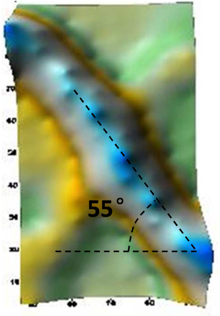
The measured shear band inclination angle.

Table 2.

The measured values and the classical solution values of shear band inclination angles.

D _r (%)	$d_{50}$ (mm)	Confining pressure (kPa)	Mohr–Coulomb solution	Roscoe solution	Arthur solution	Measured $θ$
60	1.5	50	64°	45°	54.5°	49°
		100				48°
		150				48°
	0.75	50	65°	45°	55°	57°
		100				56°
		150				55°
	0.23	50	67°	45°	56°	59°
		100				58°
		150				57°
30	1.5	50	66°	45°	55.5°	52°
		100				49°
		150				47°
	0.75	50	65°	45°	55°	53°
		100				52°
		150				50°

It can be seen that the measured inclination angles decrease as confining pressure or d₅₀ increases for the same D_r. Han and Drescher⁷ also concluded that $θ$ values decrease as the confining pressure increases. Generally, Table 2 shows that the measured shear band orientation angle is closer to Arthur solution. Finno et al.¹⁰ concluded that the measured $θ$ lies between the Coulomb and Arthur solutions for a loose, fine-grained sand. Alshibli and Sture¹⁹ observed that the confining pressure had different influences on $θ$ for different sand. Moreover, they thought that the Roscoe solution gave good predictions, whereas the Coulomb solution overestimated these values.

The characteristics of stress–strain curves for different parts of the specimen

The characteristics of the stress–strain curves for the whole sample and the point inside the shear band

In this study, the sand sample has the relative density of 60%, the mean particle size of 0.75 mm. During the test, the CMOS camera will collect the data of four corner points for each white square. The deformation of a total of 128 corner points for 32 squares is collected. The corner points are ranked and numbered from top to bottom. The 53rd point, the 47th point, and the 43rd point are selected to study the characteristics of the stress–strain for local points in the specimen under the confining pressures of 50, 100, and 150 kPa, respectively. It should be noted that the stress is approximately obtained by the load divided by the cross-sectional area of the point due to the incapability of obtaining the stress for interior point at present. Figure 18(a)–(c) gives the final deformation of the samples and the relationships between stress difference and axial strain of the whole sample and of these three points inside the shear band, respectively.

Figure 18.

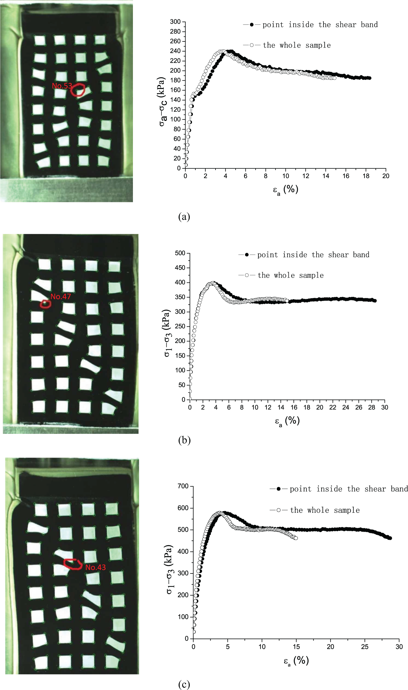
Relationships between stress differences and axial strain of the whole sample and the interior point: (a) $σ_{c} = 50 kPa$ , (b) $σ_{c} = 100 kPa$ , and (c) $σ_{c} = 150 kPa$ .

From Figure 18, it can be seen that the relationship between the stress difference and the axial strain of the local points is similar to that of the whole sample. Before reaching the peak strength, the two curves basically coincide, and the stress difference of the sample increases with increasing axial strain, which is known as the strain hardening stage. As the test continues, the phenomenon of softening occurs as the axial strain increases gradually. The softening of the total sample is presented more clearly than that of the interior point, while the axial strain of the interior point is larger than that of the whole sample at the end of the test. Especially, the higher the confining pressure, the larger the axial strain difference between these two cases. The reason lies in that the shear band and softening stage occur earlier for higher confining pressure, and the axial strain is concentrated in the shear band and in the softening stage, whereas the axial strain in other parts is small and even unloading rebound. The axial strain of the whole sample reflects the mean strain, which is far smaller than the strain actually generated in the shear band.

The characteristics of stress–strain curves for the points inside and outside the shear band

In this study, the sand sample is the same as that in section “The characteristics of the stress–strain curves for the whole sample and the point inside the shear band.”Figure 19(a)–(c) gives the final deformation of the samples and the relationships between stress difference and axial strain of the points inside and outside the shear band under the confining pressures of 50, 100, and 150 kPa, respectively.

Figure 19.

Relationships between stress differences and axial strain of points inside and outside the band: (a) $σ_{c} = 50 kPa$ , (b) $σ_{c} = 100 kPa$ , and (c) $σ_{c} = 150 kPa$ .

Also, Figure 19 shows that the stress difference in the sample increases with increasing axial strain until the stress difference reaches the peak value.

From Figure 19, it can be seen that the stress–strain relationship is roughly a straight line until the stress reaches its peak value for points outside the shear band, while the stress–strain relationship for the point in the shear band is linear when the axial strain is small and then grows with nonlinearity until the peak value is reached. Also, it can be seen that the strain in the shear band is larger than that outside the shear band at the peak value. After the peak value, the stress in the shear band decreases slowly, whereas the stress outside the shear band drop dramatically; that is, the strain inside the shear band increases dramatically at the softening stage, whereas the strain outside the shear band almost stops increasing and even behaves elastic unloading rebound. The phenomenon reflects the continuing growth of unrecoverable plastic deformation for the sand in the shear band while almost elastic deformation for the sand outside the shear band.

In addition, from the above analysis, it can be seen that there is much difference in the stress–strain relationship for the different parts in the sample, especially after the peak value. In this case, the sample behaves like an uneven structure instead of an even element. It means that our usual method for measuring the stress–strain relationship of the soil sample with a plane strain test is only a macroscopic approximation, which may not be appropriate to be used for determination the constitutive law of the soil. Recently, Shao et al.³³ gave the similar results for the triaxial test.

Conclusion

In this article, a new type of plane strain apparatus is introduced. It has two typical characters, that is, flexible loading for lateral confining pressure and the digital image technique for surface deformation measurement. The digital image measurement based on corner detection is powerful in noncontact measurement and accurate enough in deformation measurement. With this technique, the strain of the local points and the whole deformation process of the sample can be obtained, which are used to analyze the mechanical characteristics of the sand and the formation process of the shear band under the condition of plane strain. The following conclusions can be drawn:

The curve of the stress difference and axial strain has three obvious stages, that is, the hardening stage, the softening stage, and the residual stage. During the testing process, the specimen is expanded in the horizontal direction and the expansion rate of the sample is kept constant.

The bifurcation point of the curves between lateral strain and axial strain can be used to detect the starting point of strain localization. The smaller the confining pressure, the smaller the particle size, and the higher the relative density, the earlier the strain localization takes place.

The development of the shear band starts before the peak value of the stress–strain curve and forms after the peak value. The sand with high relative density has a clear peak value and softening stage.

The measured inclination angles decrease as confining pressure or the mean size increases for the same relative density. Generally, the measured shear band orientation angle is closer to Arthur solution.

The strain inside the shear band increases dramatically at the softening stage, whereas it almost stops increasing and even behaves elastic unloading outside the shear band. It means that there is continuing growth of unrecoverable plastic deformation in the shear band while almost elastic deformation outside.

In the study, the sand sample behaves like an uneven structure instead of an even element. Our usual method for measuring the stress–strain relationship of the soil sample with a plane strain or triaxial test is only a macroscopic approximation. For granular material, the relevant parameters of the constitutive model may be determined by combination of microscopic observations and the connection and transformation of the physical parameters from micro–macro two-scale analysis based on the average field theory.^35,36

Footnotes

Handling Editor: Hongyan Ma

Declaration of conflicting interests

The author(s) declared no potential conflicts of interest with respect to the research, authorship, and/or publication of this article.

Funding

The author(s) disclosed receipt of the following financial support for the research, authorship, and/or publication of this article: This work was financially supported by National Key R&D Program of China (2016YFE0200100), the State Key Laboratory of Geohazard Prevention and Geoenvironment Protection (SKLGP2017K023), the National Natural Science Fund of China (51678112), and the Fundamental Research Funds for the Central Universities (DUT16ZD211).

References

Hambly

. A new true triaxial apparatus. Geotechnique 1969; 19(2): 307–309.

Finn

WDL

Wade

Lee

KL.

Volume changes in triaxial and plane strain tests. J Soil Mech Found 1967; 93(6): 297–308.

Kirkparick

Belshaw

DJ.

On the interpretation of the triaxial test. Geotechnique 1968; 18(3): 336–350.

Arthur

JRF

Dunstan

. Rupture layers in granular media. In: Proceedings of the IUTAM conference on deformation and failure of granular materials (eds Vermeer

Luger

), Delft, 31 August–3 September, 1982, pp.453–459.

Desrues

Lanier

Stutz

Localization of the deformation in tests on sand sample. Eng Fract Mech 1985; 21(4): 909–921.

Han

Vardoulakis

Plane strain compression experiments on water-saturated fine-grained sand. Geotechnique 1991; 41(1): 49–78.

Han

Drescher

Shear bands in biaxial tests on dry coarse sand. Soils Found 1993; 33(1): 118–132.

Desrues

Chambon

Mokni

et al . Void ration evaluation inside shear bands in triaxial sand specimens studied by computed tomography. Geotechnique 1996; 46(3): 529–546.

Finno

Harris

Mooney

MA.

Strain localization and undrained steady state of sand. J Geotech Eng 1996; 122(6): 462–473.

10.

Finno

Harris

Mooney

et al . Shear bands in plane strain compression of loose sand. Geotechnique 1997; 47(1): 149–165.

11.

Mooney

Viggiani

Finno

RJ.

Undrained shear band deformation in granular media. J Eng Mech: ASCE 1997; 123: 577–585.

12.

Mooney

Finno

Viggiani

MG.

A unique critical state for sand. J Geotech Geoenviron 1998; 124(11): 1100–1108.

13.

Yasin

SJM

Tosuoka

. Stress history-dependent deformation characteristics of dense sand in plane strain. Soils Found 2000; 40(2): 77–98.

14.

Desrues

Viggiani

Strain localization in sand: an overview of the experimental results obtained in Grenoble using stereophotogrammetry. Int J Numer Anal Met 2004; 28: 279–321.

15.

Wanatowski

Chu

Stress-strain behavior of a granular fill measured by a new plane-strain apparatus. Geotech Test J 2005; 29(2): 1–9.

16.

Sadrekarimi

Olson

SM.

Shear band formation observed in ring shear tests on sandy soils. J Geotech Geoenviron 2010; 136(2): 366–375.

17.

Harris

Viggiani

Mooney

MA.

Use of stereophotogrammetry to analyze the development of shear bands in sand. Geotech Test J 1995; 18: 405–420.

18.

Liang

Saada

Figueroa

JL.

The use of digital image processing in monitoring shear band development. Geotech Test J 1997; 20: 324–339.

19.

Alshibli

Sture

Shear band formation in plane strain experiments of sand. J Geotech Geoenviron 2000; 126(6): 495–503.

20.

Alshibli

Sture

Costes

NC.

Assessment of localized deformations in sand using X-ray computed tomography. Geotech Test J 2000; 23: 274–299.

21.

Alshibli

Batiste

Sture

Strain localization in sand: plane strain versus triaxial compression. J Geotech Geoenviron 2003; 129(6): 483–494.

22.

Takahashi

Oda

Takemura

Microstructure in shear band observed by microfocus X-ray computed tomography. Geotechnique 2005; 55(4): 333–335.

23.

Alshibli

Hasan

Spatial variation of void ratio and shear band thickness in sand using X-ray computed tomography. Geotechnique 2008; 58: 249–257.

24.

Borja

Song

Rechenmacher

et al . Shear band in sand with spatially varying density. J Mech Phys Solids 2013; 61: 219–234.

25.

Peters

Ranson

WF.

Digital imaging techniques in experimental stress analysis. Opt Eng 1982; 21(3): 427–431.

26.

Pan

Qian

Xie

et al . Two-dimensional digital image correlation for in-plane displacement and strain measurement: a review. Meas Sci Technol 2009; 20(6): 062001.

27.

Rechenmacher

Finno

RJ.

Digital image correlation to evaluate shear banding in dilative sands. Geotech Test J 2004; 27: 13–22.

28.

Rechenmacher

Chupin

Abedi

Evolution of force chains in shear bands in sands. Geotechnique 2010; 60: 343–351.

29.

Rechenmacher

Abedi

Chupin

Characterization of mesoscale instabilities in localized granular shear using digital image correlation. Acta Geotech 2011; 6: 205–217.

30.

Chupin

Rechenmacher

Abedi

Finite strain analysis of nonuniform deformations inside shear bands in sands. Int J Numer Anal Met 2012; 36(14): 1651–1666.

31.

Take

WA.

Thirty-sixth Canadian geotechnical colloquium: advances in visualization of geotechnical processes through digital image correlation. Can Geotech J 2015; 52(9): 1199–1220.

32.

Sutton

Orteu

Schreier

Image correlation for shape, motion and deformation measurements: basic concepts, theory and applications. New York: Springer, 2009.

33.

Shao

Liu

Zeng

et al . Recognition of the stress-strain curve based on the local deformation measurement of soil specimens in the triaxial test. Geotech Test J 2016; 39: 658–672.

34.

. The error correction and data processing of digital image measurement based on plane strain experiment. Doctoral Thesis. Dalian University of Technology, Dalian, 2013.

35.

Ehlers

Ramm

Diebels

et al . From particle ensembles to Cosserat continua: homogenization of contact forces towards stress and couple stresses. Int J Solids Struct 2003; 40: 6681–6702.

36.

Andrade

Avila

Hall

SA.

Multiscale modeling and characterization of granular matter: from grain kinematics to continuum mechanics. J Mech Phys Solids 2011; 59: 237–250.

A plane strain testing apparatus characterized by flexible loading and noncontact deformation measurement and its application to the study of shear band failure of sand

Abstract

Keywords

Introduction

The new type of plane strain testing apparatus

Components of the plane strain apparatus

The pressure cell

The loading system

The measurement system

The strain calculation

Testing process

The testing materials

Study on the mechanical properties of sand based on the plane strain test

The relationship between the stress difference and the axial strain

The relationship between axial strain and lateral strain

Relationship between the volume strain and the equivalent strain

The analysis for the characteristics of the shear band

Determination of the initial strain for the strain localization

Analysis of the formation of the shear band based on the shear strain field

Inclination angle of shear band

The characteristics of stress–strain curves for different parts of the specimen

The characteristics of the stress–strain curves for the whole sample and the point inside the shear band

The characteristics of stress–strain curves for the points inside and outside the shear band

Conclusion

Footnotes

Declaration of conflicting interests

Funding

References