Charge critical sensors first: Minimize data loss in wireless rechargeable sensor networks

Abstract

In this article, we study the scheduling of a charging vehicle to replenish sensor energy in a large-scale wireless sensor network, by utilizing the novel wireless energy transfer technology. We note that existing studies do not treat different sensors in the network discriminatively and consider only how to charge as many sensors as possible before their energy expirations. However, there are some critical sensors in the network, so that many other sensors have no alternative routing paths to upload their sensing data to the base station if the critical sensors die. Therefore, the energy expiration of a critical sensor will result in that not only the sensor itself cannot continue its monitoring task, but also many other sensors cannot send their data during the dead period of the critical sensor. Then, the monitoring quality of the sensor network will significantly deteriorate due to the energy expirations of the critical sensor. Unlike existing studies, we take into account the impact of energy depletions of critical sensors and investigate a charging scheduling problem for sensor networks, which is to schedule a charging vehicle to replenish a set of to-be-charged sensors, such that not only the amount of lost data by dead sensors is minimized, but also the traveling cost of the vehicle for charging sensors is minimized, too. We then propose a novel algorithm for the problem. We finally compare the proposed algorithm with existing studies and simulation results show that the amount of lost data by the proposed algorithm is only about 50% of those by the existing studies, and the weighted sum of the amount of lost data and the vehicle travel distance is about 70% of those by the existing ones.

Introduction

Wireless sensor networks (WSNs) have wide applications in forest fire monitoring, building health monitoring, marine monitoring, human health monitoring, and so on.^1–4 As sensors in conventional WSNs are mainly powered by batteries, ⁵ their limited battery capacities hinder the wide deployment of WSNs.^6,7

A recent breakthrough technique revolutionizes the way of replenishing energy to WSNs. Kurs et al. ⁸ showed that they could efficiently transmit energy wirelessly, based on the strongly coupled resonance. Researchers then proposed to employ charging vehicles to replenish sensor energy via wireless energy transfer. ⁹

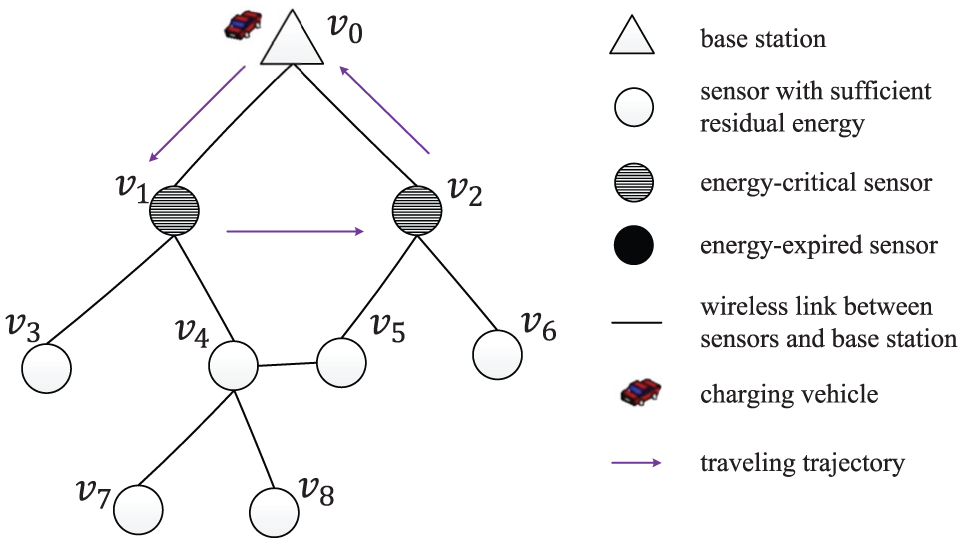
Once a sensor runs out of its energy, it cannot process its sensing tasks and transmit data to the base station. Existing studies considered to charge lifetime-critical sensors by their residual lifetimes.^2,3,10–14 For example, consider the sensor network in Figure 1, which consists of one base station $v_0$ , four sensors $v_1,v_2,v_3,\mathrm{and}{v}_4$ , and one charging vehicle. Both sensors $v_1$ and $v_2$ can send their sensing data to the base station directly. But sensors $v_3$ and $v_4$ need to forward their data to sensor $v_1$ , and then sensor $v_1$ forwards the data to the base station. Assume that each sensor generates data at the same rate (e.g. $1\mathrm{kbps}$ ), and both sensors $v_1$ and $v_2$ are lifetime-critical and require to be charged, where sensor $v_2$ has run out of its energy and the residual lifetime of sensor $v_1$ is only 0.1 h. Also, assume that it will take 1 h for the charging vehicle to fully charge either of the two sensors $v_1$ and $v_2$ . Following existing charging methods,^2,3,10–14 sensor $v_2$ will be charged before sensor $v_1$ , since the residual lifetime of sensor $v_2$ is shorter than that of sensor $v_1$ (i.e. $l_2=0<l_1=0.1\mathrm{h}$ ). Then, sensor $v_1$ will wait for 1 h before the charging vehicle starts to replenish energy to it, and its dead duration is $0.9(=1-0.1)\mathrm{h}$ . Also, it can be seen that both sensors $v_3$ and $v_4$ cannot upload their sensing data to the base station during the energy depletion period of sensor $v_1$ . Then, the amount of lost data in the network is $1\mathrm{kbps}\times 0.9\mathrm{h}\times 3+0=9.72\mathrm{MB}$ .

Figure 1.

An example of a critical sensor $v_1$ .

We note that some sensors play a critical role in the data collection of sensors in the network, because of their locations. The sensors close to the base station need to relay a large amount of data for other sensors which are far away from the base station. Not only a critical sensor cannot continue its monitoring task when it depletes its energy, but also some other live sensors cannot upload their sensing data to the base station via the data relay of the sensor. For example, consider the critical sensor $v_1$ in Figure 1, where the sensors $v_3$ and $v_4$ cannot upload their data to the base station if sensor $v_1$ dies. We now consider the impact of the energy depletion of critical sensor $v_1$ . We can charge critical sensor $v_1$ first, followed by charging sensor $v_2$ . Then, sensors $v_1$ , $v_3$ , and $v_4$ can continue to upload their data to the base station without any energy depletions, while $v_2$ will deplete its energy for 1 h. Therefore, the network will lose data for $0+1\mathrm{kbps}\times 1\mathrm{h}=3.52\mathrm{MB}$ , which is much less than the amount of lost data in the existing studies (i.e. $3.52\mathrm{MB}<9.72\mathrm{MB}$ ).

From the example shown in Figure 1, it can be seen that it is not enough to just consider the residual lifetimes of sensors for charging scheduling, and the energy expiration of a critical sensor may result in that many other sensors cannot upload their monitoring data to the base station. Then, a large amount of data will be lost. The monitoring quality of WSNs will seriously deteriorate, which may incur severe consequences. For example, in a sensor network for monitoring forest fires, the energy expiration of a critical sensor prevents other sensors from uploading their data to the base station, which contains the information of detecting an early forest fire. The fire may become uncontrollable.

In this article, we take the impact of the energy expirations of critical sensors into consideration. By considering the amount of lost sensor data and the travel distance of the charging vehicle, we propose an algorithm for effective sensor charging schedulings.

The contributions of this article can be summarized as follows:

1. To the best of our knowledge, this is the first work that considers the impact of energy depletions of critical sensors when scheduling charging vehicles to replenish sensors. We formulate a novel problem, which is to find a charging tour for the charging vehicle so that both the amount of lost data of sensors and the travel distance of the charging vehicle are minimized.

2. We then calculate the amounts of lost data of sensors by a given charging tour, when the sensor network adopts a static routing protocol or a dynamic routing protocol, respectively.

3. We also propose a novel algorithm for finding an effective sensor charging tour for the vehicle.

4. We finally evaluate the proposed algorithm with extensive simulations. The simulation results show that the proposed algorithm outperforms the existing algorithms. Especially, the amount of lost data by the proposed algorithm is about 50% of those by the existing algorithms, and the weighted sum of the amount of lost data and the vehicle travel distance is about 70% of those by the existing ones.

The rest of the article is organized as follows. Section “Related works” reviews the related work. Section “Preliminaries” introduces the network model and defines the problem. Section “Calculating the amounts of lost data under static routing and dynamic routing” computes the amounts of lost data for a given charging tour, when the sensor network adopts a static or a dynamic routing protocol, respectively. Section “Heuristic algorithm” proposes a heuristic algorithm for sensor charging schedulings. Section “Performance evaluation” evaluates the performance of the proposed algorithm and section “Conclusion” concludes this article.

Related works

In recent years, wireless energy transfer has drawn a lot of attention, and researchers studied the employment of charging vehicles to charge sensors so as to prolong the lifetime of sensor networks.^{2,3,9–12,15–20} Some scientists conducted researches on the charging vehicle scheduling when only one vehicle is employed. For example, Fu et al. ¹⁰ dispatched a charging vehicle to charge only hungry sensors in each round. Peng et al. ¹¹ designed a system for sensor energy replenishment via wireless energy transfer by employing a charging vehicle in the network. But the system is only applicable for small sensor networks. Xie et al. ²¹ dispatched a charging vehicle to replenish every sensor in a sensor network in a periodical manner. They aimed to find a charging tour to maximize the ratio of the vacation time of the vehicle to its charging cycle. Ren et al. ¹⁹ studied a problem of maximizing the charging throughout. That is, a charging vehicle charges the maximum number of sensors within a given period. However, this charging strategy may incur that some remote dead sensors cannot be charged for a long time. Angelopoulos et al. ²² considered the importance of a sensor as the amount of data served by the sensor, but they ignored the fact that other live sensors may have alternative routing paths to upload their data to the base station.

There are also some researches that dispatched multiple charging vehicles for replenishing sensors. For example, Wang et al. ¹² and Gao et al. ²³ proposed a method to find the minimum number of charging vehicles and found the charging tours for the vehicles, such that the difference between the energy charged to sensors and the energy consumption on the vehicle movement is maximized. Dai et al. ¹⁵ investigated the problem of dispatching the minimum number of vehicles to charge sensors. Jiang et al. ¹⁶ studied maximizing the coverage utility of the sensor network through scheduling multiple charging vehicles to charge sensors. Xu et al.^2,3 proposed an approximation algorithm to schedule multiple charging vehicles to replenish sensors for an entire monitoring period, so that the total travel distance of the vehicles for the period is minimized, by considering the different energy consumption rates of different sensors.

In addition, a breakthrough can realize ultra-fast charging using a lithium iron phosphate material, which can reach a charging rate of $400\mathrm{C}/\mathrm{s}$ . ²⁴ Then, a sensor will be fully replenished within a few seconds, and the charging time can thus be neglected. Based on this technology, Lu et al. ¹⁸ proposed a collaborative charging model, in which vehicles can transfer energy to each other. They studied the problem of scheduling vehicles to charge sensors, so that the ratio of the payload energy to the overload energy is maximized. Liang et al. ¹⁷ deployed multiple charging vehicles with an on-demand strategy in a two-dimensional (2D) space. They found the minimum number of vehicles to charge sensors under the energy capacity constraint on each vehicle. These researches do not take the sensor charging time into account due to the high-speed charging rate. However, it is still very expensive to adopt the ultra-fast battery materials in sensors.

Different from the existing studies that ignored different impacts of the energy expirations of different sensors, we distinctively treat sensors by the amount of lost data due to their energy depletions. When a critical sensor depletes its energy, the network may lose a large amount of data. In this article, we jointly consider the impact of the energy expirations of critical sensors and the travel distance of the charging vehicle to schedule the charging vehicle.

Preliminaries

In this section, we first present the network model and then introduce static routing and dynamic routing. We finally define the problem precisely.

Network model

We consider a of WSN deployed in a 2D space with $n_s$ sensors $v_1,v_2,\dots ,v_{n_s}$ , and each sensor $v_i$ is powered by a rechargeable battery with energy capacity $B_i$ . There is a base station $v_0$ in the network located at the center for gathering sensing data from the $n_s$ sensors. Denote by $V_s$ the set of sensors and the base station, that is, $V_s=\{v_0,v_1,v_2,\dots ,v_{n_s}\}$ .

Each sensor $v_i$ generates its data at a rate of $r_i$ . It uploads its sensing data to the base station directly or forwards its data to another sensor which is closer to the base station. Denote by $G_s$ the data transmission graph, that is, $G_s=(V_s,E_s)$ , where $E_s$ indicates the set of wireless links between sensors. An edge $e_{\mathrm{ij}}$ between two nodes $v_i$ and $v_j$ is contained in $E_s$ if their Euclidean distance is within their communication range.

Two types of routing protocols

Due to the limited communication range of sensors, a sensor that is far away from the base station needs the data relay of another sensor which is close to the base station. We will consider two scenarios, one is that the sensor network adopts a static routing protocol and the other is that the network adopts a dynamic routing protocol. ²⁵ On the one hand, when the network adopts a static routing protocol, the routing path of each sensor does not change during the monitoring period of the sensor network. Then, if a sensor $v_i$ runs out its energy, those sensors which upload their data via the relay of sensor $v_i$ need to wait for the renewal of sensor $v_i$ and then continue uploading their data. As shown in Figure 2(a), sensors $v_3$ and $v_4$ cannot upload their monitoring data if sensor $v_1$ depletes its energy. Then, the data from sensors $v_1$ , $v_3$ , and $v_4$ are lost when sensor $v_1$ is dead, which is illustrated in Figure 2(b).

Figure 2.

Comparison of static routing and dynamic routing: (a) a senson network, (b) static routing, and (c) dynamic routing.

On the other hand, if the network adopts a dynamic routing protocol, once a sensor dies, the protocol will update the routing paths to adapt to the real-time change of the network topology, by finding alternative paths which consist of only live sensors. For example, in Figure 2(c), when sensor $v_1$ depletes its energy, sensor $v_4$ still can upload its data via the relay of sensor $v_5$ , since the distance between sensors $v_4$ and $v_5$ is within their communication range. The energy expiration of sensor $v_1$ impacts only the data uploading of sensor $v_3$ .

Energy consumption model

Each sensor $v_i$ has an energy capacity of $B_i$ , and it consumes its energy on data sensing, data reception, and data transmission. Then, the energy consumption rate ${\rho }_i$ of sensor $v_i$ is

$${\rho }_i=P_{sens}+P_{recv}+P_{trans}$$

(1)

where $P_{\mathrm{sens}}$ , $P_{\mathrm{recv}}$ , and $P_{\mathrm{trans}}$ are the energy consumption rates on data sensing, data reception, and data transmission, respectively, which are calculated as follows

$$P_{sens}={\sigma }_i·r_i$$

(2)

$$P_{recv}={\gamma }_i·r_i^R$$

(3)

$$P_{trans}=({\varphi }_i^1+{\varphi }_i^2\ast w_{ij}^{ϵ})·r_i^T$$

(4)

where $w_{\mathrm{ij}}$ is the Euclidean distance between sensors $v_i$ and $v_j$ ; $r_i$ , $r_i^R$ , and $r_i^T$ are the data sensing rate, the data reception rate, and the data transmission rate of sensor $v_i$ , respectively; $\sigma$ , $\gamma$ , ${\varphi }_1$ , and ${\varphi }_2$ are the given constants, and their values are $\sigma =60*{10}^{-9}\mathrm{J}/\mathrm{b}$ , $\gamma =135*{10}^{-9}\mathrm{J}/\mathrm{b}$ , ${\varphi }_1=45*{10}^{-9}\mathrm{J}/\mathrm{b}$ , $ϵ=2\mathrm{or}4$ , and ${\varphi }_2=10*{10}^{-12}\mathrm{J}/\mathrm{b}/{\mathrm{m}}^2$ , if $ϵ=2$ , and ${\varphi }_2=1*{10}^{-15}\mathrm{J}/\mathrm{b}/{\mathrm{m}}^4$ if $ϵ=4$ . ²⁶

An on-demand charging paradigm

We adopt a flexible on-demand charging paradigm to charge sensors. We assume that the energy consumption rate of each sensor is allowed to change over time. The assumption is valid in many real WSN applications, including target tracking and environmental monitoring. For example, in a WSN for event detections, if no events happen in the monitoring area of the WSN, sensors usually perform their duty cycles to save energy, and thus they can run much longer than that in wake-up statuses. When an event does occur, the sensors within the event region will be activated, and they will remain in wake-up statuses to capture the event and report their sensing results to the base station. Their wake-up statuses continue until the event is gone. Thus, the energy consumption rates of these sensors in the wake-up statues are much faster compared with those perform duty-sleep cycling ones.

Denote by $R{E}_i(t)$ the amount of residual energy of sensor $v_i$ at time $t$ . Then, the residual lifetime of sensor $v_i$ is $R{T}_i(t)=R{E}_i(t)/{\rho }_i$ . Assume that when the residual lifetime $R{T}_i(t)$ of sensor $v_i$ falls below a given threshold $\theta$ (e.g. 2 h), sensor $v_i$ will send a charging request to the base station. Then, we have a set $V$ of to-be-charged sensors at time $t$ , that is, $V=\{v_i|v_i\in V_s,R{T}_i(t)\le q·\theta \},V\subset V_s$ , where $q$ is a given constant with $q\ge 1$ . After the base station receives the charging requests, it will deploy the charging vehicle to charge the sensors in $V$ . Assume that the base station invokes a charging scheduling algorithm to obtain a charging tour $C$ for the charging vehicle, where the algorithm will be shown later. Assume that the charging tour is $C=v_0\to v_1\to v_2\to \cdots \to v_n\to v_0$ .

It can be seen that, a critical sensor $v_i$ cannot continue its monitoring task during its dead period, and many other live sensors lose their data, if they have no alternative routing paths to send their sensing data to the base station. Given a charging tour $C$ for a set $V$ of to-be-charged sensors, denote by $D_{\mathrm{loss}}^{\mathrm{static}}$ and $D_{\mathrm{loss}}^{\mathrm{dynamic}}$ the amounts of lost data under static routing and dynamic routing, respectively, and their calculations will be shown later in section “Calculating the amounts of lost data under static routing and dynamic routing.” For simplicity, denote by $D_{\mathrm{loss}}$ the amount of lost data by a given charging tour $C$ , where $D_{\mathrm{loss}}=D_{\mathrm{loss}}^{\mathrm{static}}$ if a static routing protocol is adopted; otherwise (i.e. a dynamic routing protocol is adopted) $D_{\mathrm{loss}}=D_{\mathrm{loss}}^{\mathrm{dynamic}}$ .

Denote by $L$ the total travel distance of the charging vehicle in tour $C$ , that is

$$L=w_{0,1}+w_{1,2}+\dots +w_{n,0}={\displaystyle \sum _{i=0}^n{w}_{i,i+1}}$$

(5)

where $w_{i,j}$ is the Euclidean distance between sensors $v_i$ and $v_j$ .

Problem definition

It is desirable that both the amount of lost data $D_{\mathrm{loss}}$ and the travel distance of the vehicle $L$ are minimized. On the one hand, the amount of lost data of sensors must be minimized, since the monitoring quality of the sensor network deteriorates significantly if a large amount of sensing data are lost. ²⁷ On the other hand, the travel distance of the charging vehicle must be shortened as much as possible, because a long travel distance incurs a large amount of energy consumption.^13,14

We however notice that the two objectives of minimizing both the data loss $D_{\mathrm{loss}}$ and the vehicle travel distance $L$ usually are contradictory to each other. That is, to minimize data loss, the vehicle must charge the sensors with short residual lifetimes first, even though they are far away from the vehicle; this however incurs a high vehicle travel cost. Contrarily, to shorten the vehicle travel distance, the vehicle can charge sensors along a shortest closed tour of the sensors, regardless of their residual lifetimes, but their dead durations may become much longer.

In this article, we propose a metric to measure the quality of the charging tour $C$ , which is a weighted sum of the amount of lost sensor data and the travel distance of the charging vehicle, that is

$$DL=\alpha ·D_{loss}+(1-\alpha )·L$$

(6)

where $\alpha$ is a given constant with $0\le \alpha \le 1$ . The value of $\alpha$ indicates a trade-off between the monitoring quality of the network and the energy consumption of the charging vehicle. Different applications have different requirements on the importance of sensing data. A large value of $\alpha$ indicates that a sensor network requires a high real-time data monitoring. For example, in a sensor network for early forest fire monitoring, data monitoring delay for a few hours may lead to an uncontrollable forest fire. In contrast, a small value of $\alpha$ implies that a sensor network can tolerate the data loss of sensors for some time. For instance, in a sensor network for temperature monitoring, the temperature would not change significantly in a period of 1 h.

Given a sensor network $G_s=(V_s,E_s)$ , a set $V$ of lifetime-critical sensors at some time, and a weight $\alpha$ of the amount of lost data, in this article we consider the problem of finding a charging tour $C=v_0\to v_1\to v_2\to \cdots \to v_n\to v_0$ for a charging vehicle, such that the weighted sum $\mathrm{DL}$ of the amount of lost data $D_{\mathrm{loss}}$ and the vehicle travel distance $L$ in tour $C$ is minimized, where $\mathrm{DL}=\alpha ·D_{\mathrm{loss}}+(1-\alpha )·L$ .

Calculating the amounts of lost data under static routing and dynamic routing

Given a set $V$ of to-be-charged sensors at time $t_0$ and a charging tour $C=v_0\to v_1\to v_2\to \cdots \to v_n\to v_0$ of the charging vehicle for charging sensors in $V$ , assume that the total time spent by the vehicle for charging sensors in $V$ and on its travel along tour $C$ is no more than $T$ . Then, we calculate the amount of lost data of sensors during the time interval $[t_0,t_0+T]$ .

For each sensor $v_i$ in $V$ , we find its dead interval, which is from its dead time $t_i^d$ to its start charging time $t_i^c$ if the sensor will run out of its energy. We first calculate the dead time $t_i^d$ of sensor $v_i$ . Recall that the residual lifetime of sensor $v_i$ at time $t_0$ is $R{T}_i(t_0)$ , then the dead time $t_i^d$ of sensor $v_i$ is

$$t_i^d=t_0+R{T}_i(t_0)$$

(7)

Next, we calculate the start charging time $t_i^c$ of sensor $v_i$ . Assume that the start charging time $t_{i-1}^c$ of sensor $v_{i-1}$ has been found. Before the vehicle charges sensor $v_i$ , the vehicle must fully replenish sensor $v_{i-1}$ and then travel from the location of sensor $v_{i-1}$ to the location of sensor $v_i$ . It will take $t_{v_{i-1}}$ time to charge sensor $v_{i-1}$ , where $t_{v_{i-1}}=(B_{i-1}-R{E}_{i-1}(t_{i-1}^c))/\beta$ , $B_{i-1}$ is the battery capacity of sensor $v_{i-1}$ , $R{E}_{i-1}(t_{i-1}^c)$ is the residual energy of sensor $v_{i-1}$ at time $t_{i-1}^c$ , that is, $R{E}_{i-1}(t_{i-1}^c)=max\{0,R{E}_{i-1}(t_0)-{\rho }_{i-1}(t_{i-1}^c-t_0)\}$ , and $\beta$ is the charging rate of the charging vehicle. The charging vehicle will spend $t_{i-1,i}=w_{i-1,i}/\mu$ time for moving from sensor $v_{i-1}$ to sensor $v_i$ , where $w_{i-1,i}$ is the distance between sensors $v_{i-1}$ and $v_i$ . Then, the start charging time of sensor $v_i$ is

$$t_i^c=t_{i-1}^c+t_{v_{i-1}}+t_{i-1,i}$$

(8)

It can be seen that if the start charging time $t_i^c$ of sensor $v_i$ in tour $C$ is earlier than its dead time $t_i^d$ (i.e. $t_i^c\le t_i^d$ ), the sensor will not deplete its energy. Otherwise $(t_i^c>t_i^d)$ , the sensor will run out of its energy from $t_i^d$ to $t_i^c$ . Also, we notice that a sensor cannot upload its sensing data at some time if it depletes its energy at that time, or some relay sensors on the routing path from the sensor to the base station run out of their energy. Then, in the time interval $[t_0,t_0+T]$ , sensor $v_i$ may not send its data to the base station in multiple intervals.

To calculate the amount of lost data of the sensor network, which is the sum of the amounts of lost data of the sensors in the interval $[t_0,t_0+T]$ , we distinguish our discussions into two cases: static routing and dynamic routing.

Calculating the amount of lost data under static routing

Denote by $P_i$ the data routing path from sensor $v_i$ to the base station $v_0$ , assuming that $P_i=v_i\to v_{i,1}\to v_{i,2}\to \cdots \to v_{i,k}\to v_0$ . The routing path of sensor $v_{i,1}$ (which is the parent of sensor $v_i$ in path $P_i$ ) is $P_{i,1}=v_{i,1}\to v_{i,2}\to \cdots \to v_{i,k}\to v_0$ . Then, $P_i=v_i\to P_{i,1}$ . Denote by $T_i$ the set of data-lost intervals of sensor $v_i$ , assuming that $T_i=\{[t_{i,1}^s,t_{i,1}^f],[t_{i,2}^s,t_{i,2}^f],\dots ,[t_{i,p}^s,t_{i,p}^f]\}$ , where $t_0\le t_{i,1}^s<t_{i,1}^f<t_{i,2}^s<t_{i,2}^f<\cdots <t_{i,p}^s<t_{i,p}^f\le t_0+T$ . The data-lost duration of sensor $v_i$ is thus

$$t_i={\displaystyle \sum _{j=1}^p\left(t_{i,j}^f-t_{i,j}^s\right)}$$

(9)

Assume that the set $T_{i,1}$ of data-lost intervals of sensor $v_{i,1}$ has been found, which is $T_{i,1}=\{[t_{i,1}^s,t_{i,1}^f],[t_{i,2}^s,t_{i,2}^f],\dots ,[t_{i,m}^s,t_{i,m}^f]\}$ . Then, the set $T_i$ of data-lost intervals of sensor $v_i$ consists of the dead interval of sensor $v_i$ and the set $T_{i,1}$ of data-lost intervals of subpath $P_{i,1}$ . That is

$$T_i=[t_i^d,t_i^c]\cup T_{i,1}$$

(10)

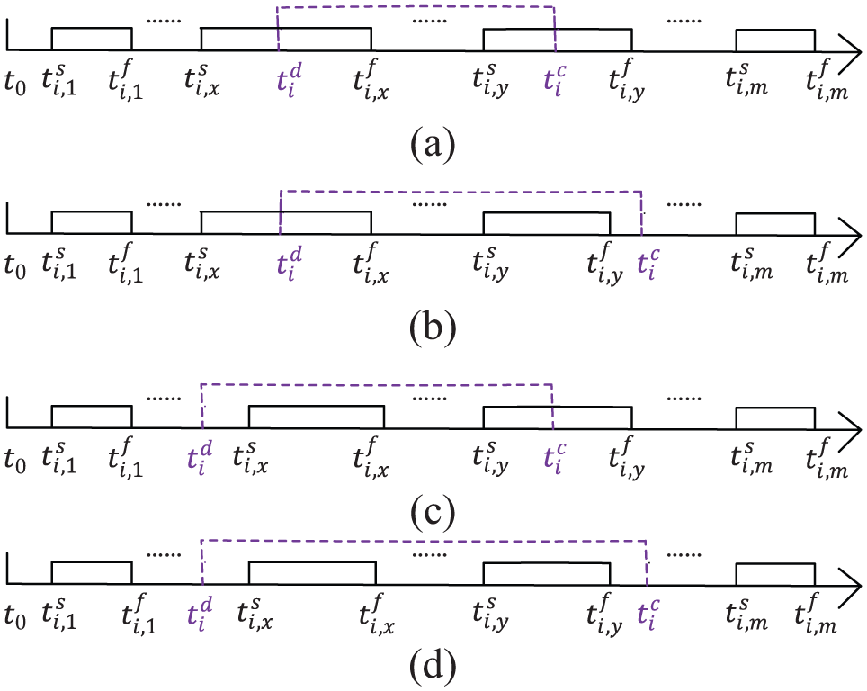
It can be seen that the dead interval $[t_i^d,t_i^c]$ of sensor $v_i$ may span multiple intervals in $T_{i,1}$ ; see Figure 3. We then calculate the set $T_i$ so that any two intervals are disjoint with each other. We consider four cases as follows.

• Case 1. $t_i^d$ is contained in an interval $[t_{i,x}^s,t_{i,x}^f]$ , and $t_i^c$ is contained in another interval $[t_{i,y}^s,t_{i,y}^f]$ , where $x$ and $y$ are two positive integers with $1\le x\le y\le p$ ; see Figure 3(a). We can remove the intervals from the $x\mathrm{th}$ interval to the $y\mathrm{th}$ interval from $T_{i,1}$ and then add a new interval $[t_{i,x}^s,t_{i,y}^f]$ . That is

$$T_i=(T_{i,1}\backslash \{[t_{i,x}^s,t_{i,x}^f],\dots ,[t_{i,y}^s,t_{i,y}^f]\})\cup [t_{i,x}^s,t_{i,y}^f].$$

• Case 2. $t_i^d$ is contained in an interval $[t_{i,x}^s,t_{i,x}^f]$ , while $t_i^c$ is not contained in any intervals in $T_{i,1}$ . Assume that $t_i^c$ is after the end time of the $y\mathrm{th}$ interval $[t_{i,y}^s,t_{i,y}^f]$ , but before the $(y+1)\mathrm{th}$ interval; see Figure 3(b). We remove the intervals from the $x\mathrm{th}$ interval to the $y\mathrm{th}$ interval from $T_{i,1}$ and then add a new interval $[t_{i,x}^s,t_i^c]$ . That is

$$T_i=(T_{i,1}\backslash \{[t_{i,x}^s,t_{i,x}^f],\dots ,[t_{i,y}^s,t_{i,y}^f]\})\cup [t_{i,x}^s,t_i^c]$$

• Case 3. $t_i^d$ is not contained in any intervals in $T_{i,1}$ , while $t_i^c$ is contained in an interval $[t_{i,y}^s,t_{i,y}^f]$ . Assume that $t_i^d$ is after the end time of the $(x-1)\mathrm{th}$ interval, but before the $x\mathrm{th}$ interval $[t_{i,x}^s,t_{i,x}^f]$ ; see Figure 3(c). We remove the intervals from the $x\mathrm{th}$ interval to the $y\mathrm{th}$ interval from $T_{i,1}$ and then add a new interval $[t_i^d,t_{i,y}^f]$ . That is

$$T_i=(T_{i,1}\backslash \{[t_{i,x}^s,t_{i,x}^f],\dots ,[t_{i,y}^s,t_{i,y}^f]\})\cup [t_i^d,t_{i,y}^f]$$

• Case 4. Both $t_i^d$ and $t_i^c$ are not contained in any intervals in $T_{i,1}$ . Assume that $t_i^d$ is after the end time of the $(x-1)\mathrm{th}$ interval but before the $x\mathrm{th}$ interval $[t_{i,x}^s,t_{i,x}^f]$ , and $t_i^c$ is after the end time of the $y\mathrm{th}$ interval $[t_{i,y}^s,t_{i,y}^f]$ but before the $(y+1)\mathrm{th}$ interval; see Figure 3(d). We remove the intervals from the $x\mathrm{th}$ interval to the $y\mathrm{th}$ interval from $T_{i,1}$ and then add a new interval $[t_i^d,t_i^c]$ . That is

$$T_i=(T_{i,1}\backslash \{[t_{i,x}^s,t_{i,x}^f],\dots ,[t_{i,y}^s,t_{i,y}^f]\})\cup [t_i^d,t_i^c]$$

Figure 3.

A new interval by joining multiple disjoint intervals $(x<y)$ : (a) Case 1, (b) Case 2, (c) Case 3, and (d) Case 4.

After obtaining the set $T_i$ of data-lost intervals of sensor $v_i$ , we can calculate the data-lost duration $t_i$ of sensor $v_i$ . Then, the amount of lost data of sensor $v_i$ is $d_i=r_i*t_i$ , where $r_i$ is the data rate of sensor $v_i$ . We finally calculate the amounts of lost data of the sensors in $V_s$ and thus obtain the total amount of lost data

$$D_{\mathrm{loss}}^{\mathrm{static}}=\sum _{i=1}^{n_s}{d}_i=\sum _{i=1}^{n_s}(r_i*t_i)$$

(11)

The algorithm for calculating the amount of lost data under static routing is presented in Algorithm 1.

Algorithm 1.

Calculating the amount of lost data under static routing.

Require: A sensor network $G_s=(V_s,E_s)$ , the transmission range $R$ between two sensors, the data rate $r_i$ , the routing path $P_i$ of each sensor $v_i$ in $G_s$ , a set $V\subseteq V_s$ of to-be-charged sensors, and the dead interval $[t_i^d,t_i^c]$ of each sensor $v_i$ in $V$ Ensure: The amount of lost data $D_{\mathrm{loss}}^{\mathrm{static}}$ 1: Construct a v0-rooted tree from the routing paths of the sensors in $G_s$ ;2:  $D_{\mathrm{loss}}^{\mathrm{static}}\leftarrow 0$ ;3: /* Perform a breadth-first search from the base station $v_0$ on the tree */4: for each sensor $v_i$ in $V_s$ do5:  Assume that sensor $v_{i,1}$ is the parent of sensor $v_i$ in the tree and the set of data-lost intervals of sensor $v_{i,1}$ is $T_{i,1}=\{[t_{i,1}^s,t_{i,1}^f],[t_{i,2}^s,t_{i,2}^f],\dots ,[t_{i,m}^s,t_{i,m}^f]\}$ ;6:  Calculate the set $T_i$ of data-lost intervals of sensor $v_i$ by the dead interval $[t_i^d,t_i^c]$ of sensor $v_i$ and the set $T_{i,1}$ of data-lost intervals of sensor $v_{i,1}$ ;7:  Calculate the data-lost duration $t_i$ of sensor $v_i$ by applying equation (9);8:   $D_{\mathrm{loss}}^{\mathrm{static}}\leftarrow D_{\mathrm{loss}}^{\mathrm{static}}+r_i·t_i$ ;9: end for10: return $D_{\mathrm{loss}}^{\mathrm{static}}$

Lemma 1

The time complexity of Algorithm 1 is $O(n^2)$ .

Proof

It can be seen that Algorithm 1 visits every node only once during the breadth-first search (BFS) on the tree, and for visiting each sensor $v_i$ it takes $O(n)$ time to calculate the set $T_i$ of data-lost intervals and data-lost duration $t_i$ of sensor $v_i$ . Then the time complexity of Algorithm 1 is $O(n^2)$ , since there are $n$ nodes in the v₀-rooted tree.

Calculating the amount of lost data under dynamic routing

Different from static routing, when the network adopts a dynamic routing protocol, the protocol will update the routing paths to adapt to the real-time change of the network topology once a sensor dies. For example, when a relay sensor on the routing path of a sensor $v_i$ dies, sensor $v_i$ can upload its data by finding an alternative path which consists of only live sensors.

Denote by $V_t$ the set of live sensors at time $t$ , $t_0\le t\le t_0+T$ . Let $G_t=(V_t,E_t)$ be the induced graph by set $V_t$ from $G_s$ , where $V_t\subseteq V_s$ . There may be multiple connected components in $G_t$ . Denote by $V_t^{\prime }$ the set of the sensors that are in the same connected component with the base station $v_0$ in $G_t$ . It can be seen that only sensors in $V{\prime }_t$ can transmit their data to the base station at time $t$ , whereas sensors in the set $V_s\backslash V{\prime }_t$ fail to upload their data to the base station.

In the following, we calculate the amount of lost data under dynamic routing. During the charging period $T$ , the network topology changes at only the moments when a sensor dies or the vehicle starts to charge a sensor, but does not change at other time points. Denote by $V\prime$ the set of sensors which will run out of their energy for some time in the interval $[t_0,t_0+T]$ , that is, $V\prime =\{v_i|v_i\in V,t_i^c>t_i^d\}$ , and the $n\prime (=|V\prime |)$ sensors in $V\prime$ will incur $2n\prime$ times of topology changes during $[t_0,t_0+T]$ . Let $t{\prime }_j$ be a dead time or a start charging time of a sensor in $V\prime$ and sort all the $2n\prime$ time points in the ascending order, $t_0\le t{\prime }_1\le t{\prime }_2\le \dots \le t{\prime }_{2n\prime }\le t_0+T$ . Then, the topology of the sensor network will change at time $t{\prime }_j$ due to the death or renewal of a sensor in $V\prime$ . We partition the interval $[t_0,t_0+T]$ into $2n\prime +1$ time intervals $[t_0,t{\prime }_1),[t{\prime }_1,t{\prime }_2),\dots ,[t{\prime }_{2n\prime },t_0+T)$ . It can be seen that the topology will not change in each of the $2n\prime +1$ intervals. Let $V_h$ be the set of live sensors in the $h\mathrm{th}$ interval $[t{\prime }_{h-1},t{\prime }_h)$ , $1\le h\le 2n\prime +1$ . Assume that $G_h$ is the induced subgraph by set $V_h$ .

We calculate the amount of lost data in the interval $[t{\prime }_{h-1},t{\prime }_h)$ as follows. Let $V{\prime }_h$ be the set of live sensors in the same connected component with the base station in $G_h$ . Then the amount of lost data during the interval $[t{\prime }_{h-1},t{\prime }_h)$ is $d_{G_h}=\sum _{v_i\in (V_s\backslash {V\prime }_h)}(r_i*t_{G_h})$ , where $t_{G_h}$ is the duration of the interval $[t{\prime }_{h-1},t{\prime }_h)$ , that is, $t_{G_h}=t{\prime }_h-t{\prime }_{h-1}$ . Finally, the amount of lost data by sensors in $[t_0,t_0+T]$ is

$$D_{\mathrm{loss}}^{\mathrm{dynamic}}=\sum _{h=1}^{2n\prime +1}{d}_{G_h}=\sum _{h=1}^{2n\prime +1}\sum _{v_i\in (V_s\backslash {V\prime }_h)}(r_i*t_{G_h})$$

(12)

The algorithm for calculating the amount of lost data under dynamic routing is presented in Algorithm 2 .

Algorithm 2.

Calculating the amount of lost data under dynamic routing.

Require: A sensor network $G_s=(V_s,E_s)$ , the transmission range $R$ between two sensors, the data rate $r_i$ of each sensor $v_i$ in $G_s$ , a set $V\subseteq V_s$ of to-be-charged sensors, and the dead interval $[t_i^d,t_i^c]$ of each sensor $v_i$ in $V$ Ensure: The amount of lost data $D_{\mathrm{loss}}^{\mathrm{dynamic}}$ 1:  $D_{\mathrm{loss}}^{\mathrm{dynamic}}\leftarrow 0$ ;2: Sort the dead time points and start charging time points of sensors in $V$ in the increasing order, assuming that $t_0\le t{\prime }_1\le t{\prime }_2\le \dots \le t{\prime }_{2n\prime }\le t_0+T$ ;3: for $h\leftarrow 1$ to $2n\prime +1$ do4:   $t_{G_h}\leftarrow t{\prime }_h-t{\prime }_{h-1}$ ; /* the duration of the $h\mathrm{th}$ interval $[t{\prime }_{h-1},t{\prime }_h)$ */5:  Find the set $V_h$ of live sensors in the interval $[t{\prime }_{h-1},t{\prime }_h)$ ;6:  Let $G_h=(V_h,E_h)$ be the induced graph by set $V_h$ from $G_s$ ;7:  Find the set $V{\prime }_h$ of sensors in $G_h$ that are in the same connected component with the base station $v_0$ ;8:   $d_{G_h}\leftarrow 0$ ; /* the amount of lost data by sensors in $G_h$ in the interval $[t{\prime }_{h-1},t{\prime }_h)$ */9:  for each sensor $v_i$ in $V_s\backslash V{\prime }_h$ do10:    $d_{G_h}\leftarrow d_{G_h}+r_i·t_{G_h}$ ;11:  end for12:    $D_{\mathrm{loss}}^{\mathrm{dynamic}}\leftarrow D_{\mathrm{loss}}^{\mathrm{dynamic}}+d_{G_h}$ ;13: end for14: return $D_{\mathrm{loss}}^{\mathrm{dynamic}}$

Lemma 2

The time complexity of Algorithm 2 is $O(n(n+m))$ .

Proof

It can be seen that the amount of lost data in $G_s$ in the interval $[t_0,t_0+T]$ is the sum of the amounts of lost data in the $2n\prime +1$ intervals. In each interval, it takes $O(m)$ time to find the sensors that are in the same connected component with $v_0$ by performing a depth-first search (DFS) from the base station $v_0$ , and it then takes $O(n)$ time to calculate the amount of lost data for sensors in $V_s\backslash V{\prime }_h$ in the $h\mathrm{th}$ interval $[t{\prime }_{h-1},t{\prime }_h]$ . Therefore, the running time of Algorithm 2 is $O(2n\prime (n+m))=O(n(n+m))$ , as $O(n\prime )=O(n)$ .

We here use an example to illustrate the calculation of the amount of lost data in the interval $[t_0,t_0+T]$ . Assume that there are two energy-critical sensors $v_1$ and $v_2$ in the network; see Figure 4. We further assume that the charging tour is $v_0\to v_1\to v_2\to v_0$ and $t_0<t_1^d<t_2^d<t_1^c<t_2^c$ , where $t_1^d$ and $t_2^d$ are the dead times of sensors $v_1$ and $v_2$ , and $t_1^c$ and $t_2^c$ are the start charging times of sensors $v_1$ and $v_2$ , respectively. We compute the amount of lost data of the network as follows.

Figure 4.

An example for calculating the amount of lost data under dynamic routing.

In the first interval $[t_0,t_1^d)$ , no sensors die and the sensor network in $[t_0,t_1^d)$ is shown in Figure 5(a). The amount of lost data during the interval is $d_{G_1}=0$ .

Figure 5.

The network topology in each interval: (a) sensor network in $[t_0,t_1^d)$ , (b) sensor network in $[t_1^d,t_2^d)$ , (c) sensor network in $[t_2^d,t_1^c)$ , (d) sensor network in $[t_1^c,t_2^c)$ , and (e) sensor network in $[t_2^c,t_0+T]$ .

In the second interval $[t_1^d,t_2^d)$ , sensor $v_1$ dies at time $t_1^d$ . Then, sensor $t_i^c>t_i^d$ is unable to upload its data to the base station, while sensor $v_4$ can upload its data via the relay of sensor $v_5$ ; see Figure 5(b). The amount of lost data in the interval $[t_1^d,t_2^d)$ is $d_{G_2}=(r_1+r_3)*t_{G_2}$ , where $t_{G_2}=t_2^d-t_1^d$ .

In the third interval $[t_2^d,t_1^c)$ , sensor $v_1$ has not been charged yet, and sensor $v_2$ expires its energy at time $t_2^d$ . All sensors cannot upload their data; see Figure 5(c). The amount of lost data in the interval $[t_2^d,t_1^c)$ is $d_{G_3}=\sum _{i=1}^8(r_i*t_{G_3})$ , where $t_{G_3}=t_1^c-t_2^d$ .

In the fourth interval $[t_1^c,t_2^c)$ , sensor $v_1$ is charged at time $t_1^c$ but sensor $v_2$ has not been charged yet. Then, sensors $v_3$ and $v_4$ can upload their data via sensor $v_1$ , and sensors $v_5$ , $v_7$ , and $v_8$ can also send their data to the base station by the relay of sensor $v_4$ . Sensor $v_6$ is still disconnected with the base station $v_0$ , since sensor $v_2$ has not been charged yet; see Figure 5(d). The amount of lost data in the interval $[t_1^c,t_2^c)$ is $d_{G_4}=(r_2+r_6)*t_{G_4}$ , where $t_{G_4}=t_2^c-t_1^c$ .

In the fifth interval $[t_2^c,t_0+T]$ , sensor $v_2$ is charged at time $t_2^c$ . All sensors are live in this interval; see Figure 5(e). The amount of lost data in this interval is $d_{G_5}=0$ .

The total amount of lost data in $[t_0,t_0+T]$ is then $\sum _{i=1}^5{d}_{G_i}$ .

Heuristic algorithm

In this section, we propose a novel heuristic algorithm for the data loss and the travel distance minimization problem. We first describe the algorithm and then devise two pruning strategies to reduce the running time of the heuristic algorithm.

Algorithm description

We propose a heuristic algorithm to find a charging tour $C$ , which has the minimum value of the objective function $\mathrm{DL}=\alpha D_{\mathrm{loss}}+(1-\alpha )L$ . Given a set $V$ of $n$ sensors, the algorithm delivers the charging tour with multiple iterations and finds the $i\mathrm{th}$ to-be-charged sensor $v_i$ in the $i\mathrm{th}$ iteration. Assume that the algorithm has found the first $i$ to-be-charged sensors $v_1,v_2,\dots ,v_i$ in the first $i$ iterations and their charging order is $v_1\to v_2\to \cdots \to v_i$ . The algorithm finds the $(i+1)\mathrm{th}$ to-be-charged sensor as follows. It can be seen that there are $A_{n-i}^k$ different sequences by choosing $k$ sensors from the rest $n-i$ sensors, where $k(\le n-i)$ is a given positive integer, for example, $k=3$ . For each of the $A_{n-i}^k$ sequences, the algorithm first calculates the objective value of the partial charging order with $k$ sensors. Then, the algorithm finds a sequence $v_{i+1},v_{i+2},\dots ,v_{i+k}$ among the $A_{n-i}^k$ sequences with the minimum value of $\mathrm{DL}$ . Finally, the $(i+1)\mathrm{th}$ to-be-charged sensor is $v_{i+1}$ . The algorithm continues until the last to-be-charged sensor is found.

We now show the calculations of the objective value $\mathrm{DL}$ for a partial order $v_{i+1}\to \cdots \to v_{i+k}$ . On the one hand, the travel distance of the charging vehicle is calculated as $L=w_{i,i+1}+\cdots +w_{i+k-1,i+k}$ . On the other hand, the amount of lost data $D_{\mathrm{loss}}$ will be calculated as follows. Note that we cannot calculate the amount of lost data by directly applying Algorithm 1 or Algorithm 2 in the previous section, since the charging sequence of the sensors in $V\backslash \{v_1,v_2,\dots ,v_{i+k}\}$ is unknown. Then, the start charging times of sensors in $V\backslash \{v_1,v_2,\dots ,v_{i+k}\}$ are unknown, too. For simplicity, we assume that the start charging time $t_j^c$ of each sensor $v_j$ in $V\backslash \{v_1,\dots ,v_{i+k}\}$ is $t_j^c=t_{i+k}^c+t_{v_{i+k}}$ , where $t_{i+k}^c$ is the start charging time of sensor $v_{i+k}$ and $t_{v_{i+k}}$ is the charging time of sensor $v_{i+k}$ . It can be seen that the time $t_j^c$ serves as the earliest start charging time of the remaining $n-i-k$ sensors in any charging order with the first $i+k$ sensors being $v_1,v_2,\dots ,v_{i+k}$ .

The heuristic algorithm is presented in Algorithm 3 .

Algorithm 3.

MDL.

Require: A graph $G_s=(V_s,E_s)$ , a set $V$ of to-be-charged sensors, a weighted parameter $\alpha$ with $0<\alpha <1$ , and a parameter $k$ Ensure: A charging tour $C$ with the minimum $\mathrm{DL}$ value1:  $C\leftarrow Ø$ ;2: for $i\leftarrow 1$ to $n-k+1$ do3:   $D{L}_{\min }\leftarrow \infty$ ; /* the minimum $\mathrm{DL}$ value so far */4:  while $p\leftarrow 1$ to $A_{n-i}^k$ do5:   Obtain the $p\mathrm{th}$ charging sequence $v_{i+1}\to v_{i+2}\to \cdots \to v_{i+k}$ ;6:   if routing is static then7:     $D_{\mathrm{loss}}=D_{\mathrm{loss}}^{\mathrm{static}}({\rho }_i,B_i,r_i,P_i,\beta )$ by invoking Algorithm 1 ;8:   else9:     $D_{\mathrm{loss}}=D_{\mathrm{loss}}^{\mathrm{dynamic}}({\rho }_i,B_i,r_i,\beta )$ by invoking Algorithm 2 ;10:   end if11:   if $\mathrm{DL}=\alpha D_{\mathrm{loss}}+(1-\alpha )L<D{L}_{\min }$ then12:     $C_{\mathrm{best}}\leftarrow v_{i+1}\to v_{i+2}\to \cdots \to v_{i+k}$ ;13:     $D{L}_{\min }\leftarrow \mathrm{DL}$ ;14:   end if15:  end while16:  Assume that $C_{\mathrm{best}}=v_{i+1}\to v_{i+2}\to \cdots \to v_{i+k}$ ;17:  if $i<n-k+1$ then18:   The $(i+1)\mathrm{th}$ to-be-charged sensor is $v_{i+1}$ in $C$ ;19:  else20:   /* $i=n-k+1$ */21:    $C_{\mathrm{best}}=v_{n-k+1}\to v_{n-k+2}\to \cdots \to v_n$ , with $i=n-k+1$ ;22:   The order of the last $k$ to-be-charged sensors in $C$ is $v_{n-k+1}\to v_{n-k+2}\to \cdots \to v_n$ ;23:  end if24: end for25: return tour $C$

Pruning strategies for finding a tour with the minimum DL value

We note that it takes a non-trivial time to calculate the objective value of $D_{\mathrm{loss}}$ for a charging sequence, that is, $O(n^2)$ if a static routing protocol is adopted (see Lemma 1), and $O(n(n+m))$ if a dynamic routing protocol is adopted (see Lemma 2). In addition, the heuristic algorithm finds the $(i+1)\mathrm{th}$ to-be-charged sensor by calculating the amounts of lost data for as many as $A_{n-i}^k$ different charging sequences in one iteration. In this subsection, we will devise two pruning strategies to reduce the running time of the heuristic algorithm as much as possible.

First pruning strategy

It can be seen that when a sensor uploads its data to the base station directly, its data-lost intervals will consist of only its dead interval. Assume that we have calculated the $\mathrm{DL}$ values of $p$ charging sequences of the total $A_{n-i}^k$ sequences in Algorithm 3 , where $1\le p\le A_{n-i}^k$ . Let $D{L}_{\min }=\underset{1\le q\le p}{min}\{D{L}_q\}$ . For the $(p+1)\mathrm{th}$ sequence $v_{i+1},v_{i+2},\dots ,v_{i+k}$ , in the first pruning strategy, we find a lower bound ${\mathrm{DL}}_{p+1}^{\mathrm{lb}}$ on $D{L}_{p+1}$ of the $(p+1)\mathrm{th}$ sequence as ${\mathrm{DL}}_{p+1}^{\mathrm{lb}}=\alpha \sum _{j=i+1}^{i+k}{r}_j(t_j^c-t_j^d)+(1-\alpha )L_{p+1}$ , assuming that sensors $v_{i+1},v_{i+2},\dots ,v_{i+k}$ send their data to the base station directly. If ${\mathrm{DL}}_{p+1}^{\mathrm{lb}}\ge D{L}_{\min }$ , we do not calculate the actual $\mathrm{DL}$ value of the $(p+1)\mathrm{th}$ sequence. It can be seen that it takes only $O(k)$ time to calculate the lower bound ${\mathrm{DL}}_{p+1}^{\mathrm{lb}}$ , while it takes $O(k(n+m))$ time to compute the actual value of $D{L}_{p+1}$ .

Second pruning strategy

We note that the $A_{n-1}^k$ charging sequences can be considered as a tree rooted at a virtual node $r$ , where the nodes on the path from the root node $r$ to each leaf node in the tree form a charging sequence, and the length of each path is exactly equal to $k$ . For example, Figure 6 illustrates such a tree when $n-i=4$ and $k=2$ . It can be seen that we can calculate the $\mathrm{DL}$ values of the $A_{n-1}^k$ sequences by performing a DFS from $r$ . Assume that we are now visiting a non-leaf node $v_{i+s}$ and we have obtained a partial charging sequence $v_{i+1},v_{i+2},\dots ,v_{i+s}$ , where the length of the partial sequence is strictly less than $k$ , that is, $1\le s<k$ . Assume that $D{L}_{\min }$ is the minimum value of the $\mathrm{DL}$ values of the charging sequences obtained so far and $D{L}_{\mathrm{part}-s}$ is the $\mathrm{DL}$ value of the partial sequence $v_{i+1},v_{i+2},\dots ,v_{i+s}$ . If $D{L}_{\mathrm{part}-s}\ge D{L}_{\min }$ , there is no need to visit the nodes in the subtree rooted at $v_{i+s}$ .

Figure 6.

An example for the second pruning strategy.

For example in Figure 6, there are 12 charging sequences from the root node to the leaf nodes. Denote by $D{L}_{12},D{L}_{13},D{L}_{14},D{L}_{21},D{L}_{23},D{L}_{24},D{L}_{31},D{L}_{32},D{L}_{34},D{L}_{41},D{L}_{42},\mathrm{and}D{L}_{43}$ the $\mathrm{DL}$ values of these sequences. Assume that we have calculated the $\mathrm{DL}$ values of the first three sequences $v_1\to v_2,v_1\to v_3$ , and $v_1\to v_4$ and that the current $D{L}_{\min }$ is $min\{D{L}_{12},D{L}_{13},D{L}_{14}\}$ . We next calculate the value of $D{L}_{\mathrm{part}-1}$ of $v_2$ . If $D{L}_{\mathrm{part}-1}\ge D{L}_{\min }$ , we do not calculate the $\mathrm{DL}$ values of the three sequences $v_2\to v_1,v_2\to v_3,v_2\to v_4$ .

Performance evaluation

In this section, we evaluate the performance of the proposed algorithm by comparing it with existing algorithms by varying some important parameters, including the network size, maximum sensor data rate, charging rate and travel speed of the charging vehicle, weight value $\alpha$ of the amount of lost data, and the parameter $k$ in the algorithm.

Simulation environment

We consider a wireless rechargeable sensor network deployed in a $500\mathrm{m}\times 500\mathrm{m}$ square. There are 100–500 sensors in the network, which are randomly deployed in the area. The battery capacity of each sensor $v_i\in V_s$ is $B_i=10.8\mathrm{kJ}$ . ⁹ Each sensor $v_i$ has a different data rate $r_i$ , which is randomly selected from an interval $[r_{\min },r_{\max }]$ , where $r_{\min }=1\mathrm{kbps}$ and $r_{\max }=10\mathrm{kbps}$ . The communication range of the two sensors is $50\mathrm{m}$ . We adopt a real sensor energy consumption model, which has been introduced in section “Energy consumption model.” A base station is located at the center of the area. A charging vehicle is deployed for charging sensors in the network, which is co-located with the base station. The vehicle charges a sensor at a rate of $\beta =5\mathrm{W}$ and moves at a speed of $\mu =5\mathrm{m}/\mathrm{s}$ . Each sensor sends a charging request to the base station when its residual lifetime is shorter than a given threshold $l_c=2\mathrm{h}$ . The monitoring period in the simulations is 1 year. The simulator was implemented in C++ and all simulations were performed on a server with an Intel^® Core^™ i7 CPU (2.9 GHz) and an 8 GB RAM. In addition, each simulation value in the figures is the average obtained with 1000 different networks with the same network size.

To evaluate the performance of the proposed algorithm minimizing data loss (MDL), we compare it with five existing algorithms, that is, traveling salesman problem (TSP), ²⁸ earliest deadline first (EDF), ²⁹ an NDN based real time wireless recharging protocol (NETWRAP),^13,14 adaptive-additive (AA), and temporal-spatial real-time charging scheduling algorithm (TSCA). ³⁰ Algorithm TSP finds a shortest charging tour to visit sensors, but does not consider the residual lifetimes of sensors. Algorithm EDF schedules the vehicle to charge sensors by their residual lifetimes in the increasing order, that is, the shorter the residual lifetime of a sensor is, the earlier the sensor is charged by the vehicle. Algorithm NETWRAP finds the next to-be-charged sensor with the minimum weighted sum of the residual lifetime of the sensor and the travel time for the vehicle moving to the sensor.^13,14 Algorithm AA selects a portion of sensors to be charged, so that each chosen sensor is charged before its energy depletion and the difference of the amount of energy charged to the chosen sensors and the energy consumption on the vehicle movement is maximized.^13,14 Finally, algorithm TSCA develops a temporal-spatial charging scheduling algorithm, which first sorts the to-be-charged sensors by their residual lifetimes in the increasing order and then adjusts the charging order to minimize the number of dead nodes while maximizing the energy efficiency for prolonging network lifetime. ²⁹

Algorithm performance

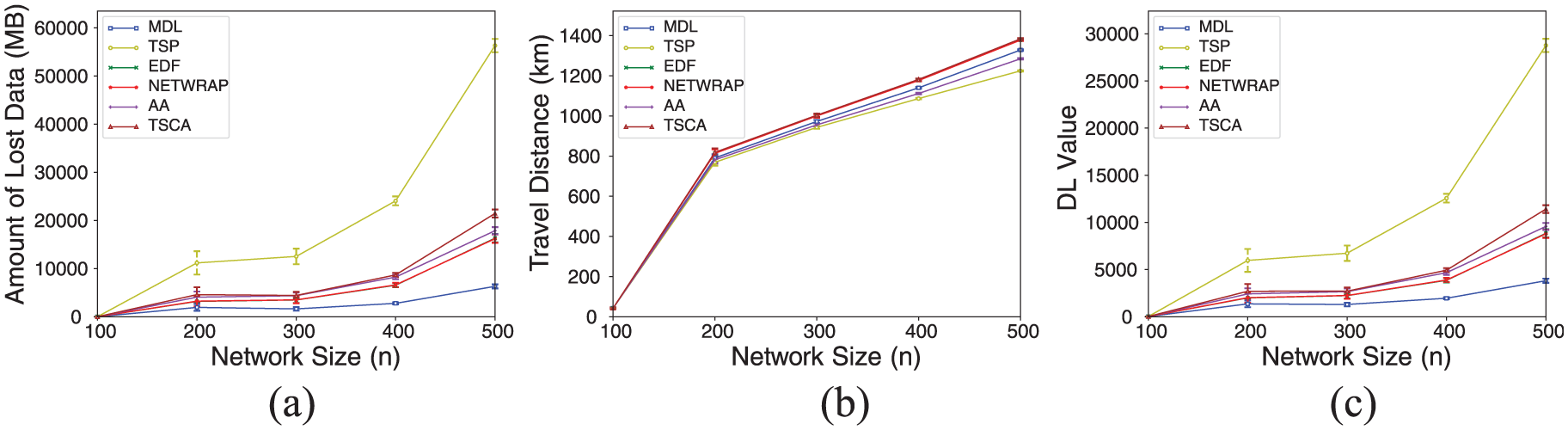
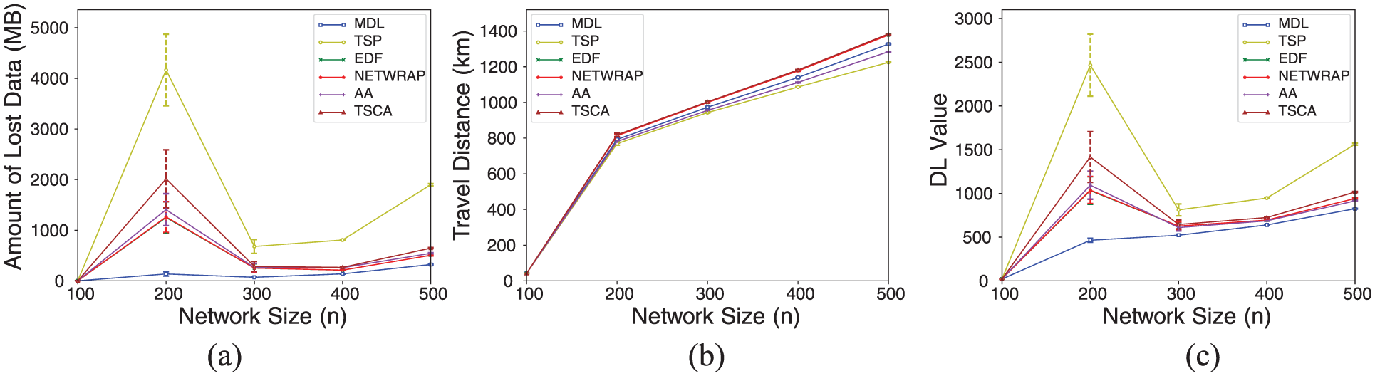
We first evaluate the performance of the proposed algorithm MDL by varying the network size from 100 to 500 under static routing and dynamic routing; see Figures 7 and 8, respectively, where $r_{\max }=10\mathrm{kbps}$ , $\beta =5\mathrm{W}$ , $\mu =5\mathrm{m}/\mathrm{s}$ , $\alpha =0.5$ , and $k=3$ . Figure 7(a) shows that, under static routing, the amount of lost data by each algorithm increases with a larger network size, and the proposed algorithm MDL delivers the smallest amount of lost data among the algorithms. For example, the amount of lost data by algorithm MDL is only about 11%, 39%, 39%, 35%, and 29% of those by the algorithms TSP, EDF, NETWRAP, AA, and TSCA, respectively, when the network size is $n_s=500$ . Figure 7(b) shows that the travel distance by each of the six algorithms increases with the increase of the network size, and the travel distances by different algorithms are almost identical. Figure 7(c) demonstrates that the objective $\mathrm{DL}$ value by algorithm MDL is the smallest one among the six algorithms, where the $\mathrm{DL}$ value is the weighted sum of the amount of lost data and the vehicle travel distance. It can be seen from Figure 7 that the algorithm MDL performs better in a larger network. For instance, the $\mathrm{DL}$ value by algorithm MDL is only about 13%, 43%, 43%, 40%, and 33% of those by the algorithms TSP, EDF, NETWRAP, AA, and TSCA, respectively, under static routing, when the network size is $n_s=500$ .

Figure 7.

Algorithm performance by varying the network size $n$ under static routing: (a) amount of lost data, (b) travel distance, and (c) DL value.

Figure 8.

Algorithm performance by varying the network size $n$ under dynamic routing: (a) amount of lost data, (b) travel distance, and (c) DL value.

Figure 8 shows the performance of the algorithms under dynamic routing, in which a sensor can find an alternative live routing path to upload its data to the base station when some sensors deplete their energy. Figure 8(a) plots similar curves as that in Figure 7(a), but the amount of lost data by each algorithm under dynamic routing is much smaller than that under static routing, since under dynamic routing a sensor with a heavy workload does not need to wait for the renewal of dead sensors in its routing path and is able to find another live routing path for data uploading. Notice that there is an interesting phenomenon shown in Figure 8(a). That is, the amount of lost data by each algorithm when there are 200 sensors in the network is more, rather than less, than that when there are more than 200 sensors (e.g. 300 sensors) The rationale behind the phenomenon is that a sensor is more likely to find a live alternative routing path with more sensors in the network when some sensors die. However, when there are 200 sensors in the network, more other live sensors may be influenced by dead sensors even if there are few dead sensors in the network. Also, the $\mathrm{DL}$ value by algorithm MDL is the smallest under dynamic routing (see Figure 8(c)).

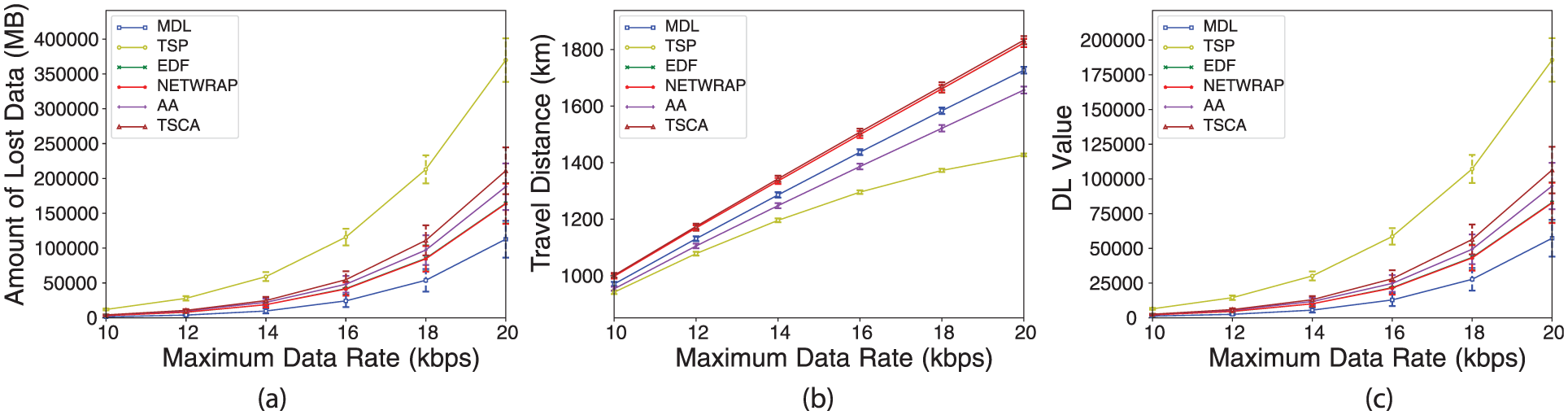
We then investigate the performance of algorithm MDL by varying the maximum data rate $r_{\max }$ from $10$ to $20\mathrm{kbps}$ , where $n_s=300$ , $\beta =5\mathrm{W}$ , $\mu =5\mathrm{m}/\mathrm{s}$ , $\alpha =0.5$ , and $k=3$ . Figures 9 and 10 demonstrate that the amounts of lost data and the $\mathrm{DL}$ values by algorithm MDL are the smallest ones among the six algorithms (see Figures 9(a) and (c) and 10(a) and (c)), and the travel distances by it are only about 4% longer than that by the state-of-the-art AA under both static routing and dynamic routing (see Figures 9(b) and 10(b)).

Figure 9.

Algorithm performance by varying the maximum data rate $r_{\max }$ under static routing: (a) amount of lost data, (b) travel distance and (c) DL value.

Figure 10.

Algorithm performance by varying the maximum data rate $r_{\max }$ under dynamic routing: (a) amount of lost data, (b) travel distance, and (c) DL value.

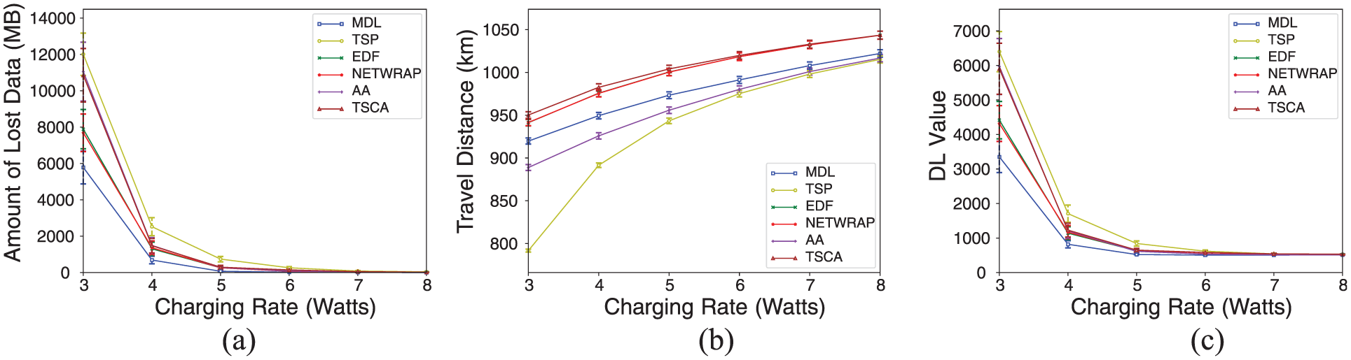
We also study the algorithm performance by varying the charging rate $\beta$ of the vehicle from $3$ to $8\mathrm{W}$ , where $n_s=300$ , $r_{\max }=10\mathrm{kbps}$ , $\mu =5\mathrm{m}/\mathrm{s}$ , $\alpha =0.5$ , and $k=3$ . Figures 11(a) and 12(a) show that the amount of lost data by each algorithm dramatically decreases with a faster charging rate, as the waiting time of each to-be-charged sensor before its charging is significantly shortened. Figures 11(b) and 12(b) demonstrate that the travel distance by each algorithm slightly increases with a faster charging rate $\beta$ , since the dead duration of each sensor is shorter with a faster charging rate $\beta$ , and its live duration is thus longer in the entire monitoring period, and the vehicle has to charge sensors more frequently. Figures 11(c) and 12(c) further show that the objective $\mathrm{DL}$ value by algorithm MDL is much smaller than that by each of the other five algorithms TSP, EDF, NETWRAP, AA, and TSCA. For instance, when the charging rate is $\beta =3\mathrm{W}$ , the $\mathrm{DL}$ value by it is about 27%, 55%, 55%, 48%, and 41% of those by the algorithms TSP, EDF, NETWRAP, AA, and TSCA under static routing and about 52%, 76%, 78%, 56%, and 57% under dynamic routing.

Figure 11.

Algorithm performance by varying the charging rate $\beta$ under static routing: (a) amount of lost data, (b) travel distance, and (c) DL value.

Figure 12.

Algorithm performance by varying the charging rate $\beta$ under dynamic routing: (a) amount of lost data, (b) travel distance, and (c) DL value.

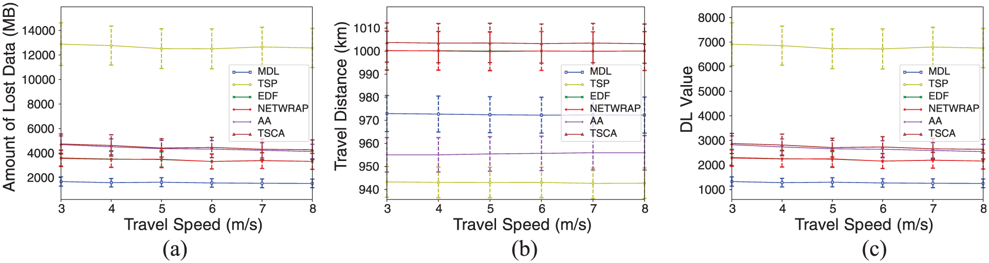
We finally investigate the algorithm performance by varying the travel speed $\mu$ of the vehicle from $3$ to $8\mathrm{m}/\mathrm{s}$ , where $n_s=300$ , $r_{\max }=10\mathrm{kbps}$ , $\beta =5\mathrm{W}$ , $\alpha =0.5$ , and $k=3$ ; see Figures 13 and 14. It can be seen that the amount of lost data and the $\mathrm{DL}$ value by algorithm MDL are the smallest ones, while its travel distance is only slightly longer than that of algorithm TSP.

Figure 13.

Algorithm performance by varying the vehicle travel speed $\mu$ under static routing: (a) amount of lost data, (b) travel distance, and (c) DL value.

Figure 14.

Algorithm performance by varying the vehicle travel speed $\mu$ under dynamic routing: (a) amount of lost data, (b) travel distance, and (c) DL value.

Impact of important parameters

We evaluate the weight $\alpha$ of the amount of lost data (see equation (6) in section “Problem definition”) on algorithm performance, by increasing $\alpha$ from 0 to 1, where $n_s=300$ , $r_{\max }=10\mathrm{kbps}$ , $\beta =5\mathrm{W}$ , $\mu =5\mathrm{m}/\mathrm{s}$ , and $k=3$ . The larger the value of $\alpha$ is, the more critical the amount of lost data is. For example, we consider only minimizing the vehicle travel cost when $\alpha =0$ , while ignoring the vehicle travel cost and considering only minimizing the amount of lost data when $\alpha =1$ . Figure 15(a) and (b) shows that both the amount of lost data and the travel distance by each of the five algorithms TSP, EDF, NETWRAP, AA, and TSCA do not change with the increase of $\alpha$ . In contrast, the amount of lost data by algorithm MDL decreases, while the travel distance by it increases, with a larger value of $\alpha$ . Figure 15(c) and 16(c) shows that the $\mathrm{DL}$ values by algorithm MDL under both static routing and dynamic routing are the smallest.

Figure 15.

Algorithm performance by varying the parameter $\alpha$ under static routing: (a) amount of lost data, (b) travel distance, and (c) DL value.

Figure 16.

Algorithm performance by varying the parameter $\alpha$ under dynamic routing: (a) amount of lost data, (b) travel distance, and (c) DL value.

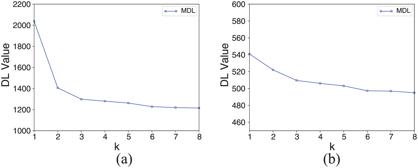
We finally study the impact of the parameter $k$ on the proposed algorithm MDL, where $k$ is the search depth in algorithm MDL for the next to-be-charged sensor. Figure 17 shows that the $\mathrm{DL}$ value by algorithm MDL is smaller with a larger value of $k$ .

Figure 17.

Algorithm performance by varying the parameter $k$ : (a) DL value under static routing and (b) DL value under dynamic routing.

In summary, it can be seen that both the amount of lost data and the objective $\mathrm{DL}$ value by algorithm MDL are much smaller than those by the other existing algorithms TSP, EDF, NETWRAP, AA, and TSCA.

Discussion

It can be seen from Figures 7–16 that the amount of lost data and the $\mathrm{DL}$ value by algorithm MDL are much smaller than those by the existing algorithms, by varying the network size, maximum sensor data rate, charging rate, vehicle travel speed, and the weight $\alpha$ of the amount of lost data. The rationale behind this is that algorithm MDL considers the impact of energy depletions of critical sensors. In algorithm MDL, critical sensors will be charged before other sensors. Then, other live sensors can continue to upload their sensing data to the base station. In contrast, sensors in the existing algorithms will be charged by only their residual lifetimes, which ignored the impact of the energy expiration of a critical sensor. When a critical sensor dies, some other live sensors may not be able to upload data, since the critical sensor plays a relay role in the data uploading of the other live sensors. Therefore, the amount of lost data by algorithm MDL is much less than those by the existing algorithms.

On the other hand, algorithm MDL considered not only the amount of lost data, but also the vehicle travel distance. Hence, the weighted sum (i.e. the $\mathrm{DL}$ value) of the amount of lost sensor data and the vehicle travel distance by algorithm MDL is much better than those by the existing algorithms.

Conclusion

In this article, we studied the scheduling of a charging vehicle in a WSN. Unlike existing studies that assumed that the impacts of the energy expirations of different sensors on the sensor network are the same, we notice that some sensors in the network play a critical role in data relay for other sensors, and their energy depletions will significantly impact the data uploading of other sensors. In this article, we take the impact of energy depletions of critical sensors into consideration. We first formulated a novel problem of finding a charging tour, such that the weighted sum of the amount of lost sensor data and the vehicle travel distance is minimized. We then calculated the amounts of lost data for a given charging tour under static routing and dynamic routing, respectively. Also, we proposed a novel algorithm for solving the problem. We finally evaluated the performance of the proposed algorithm by comparing it with the existing algorithms via extensive simulations. The simulation results showed that the proposed algorithm is very promising.