
Abstract
This article addresses information-based sensing point selection from a set of possible sensing locations. A potential game approach has been applied to addressing distributed decision making for cooperative sensor planning. For a large sensor network, the local utility function for an agent is difficult to compute, because the utility function depends on the other agents’ decisions, while each sensing agent is inherently faced with limitations in both its communication and computational capabilities. Accordingly, we propose an approximation method for a local utility function to accommodate limitations in information gathering and processing, using only a part of the decisions of other agents. The error induced by the approximation is also analyzed, and to keep the error small, we propose a selection algorithm that chooses the neighbor set for each agent in a greedy way. The selection algorithm is based on the correlation between one agent’s and the other agents’ measurement selection. Furthermore, we show that a game with an approximate utility function has an
Keywords
Introduction
The goal of cooperative sensor network planning problems is to select the sensing locations for a sensor network so that the measurement variables taken at those locations give the maximum information about the variables of interest. This problem can be formulated as an optimization problem with the global objective function of mutual information between the measurement variables and the variables of interest.1–9 For the distributed/decentralized implementation of the optimization problem, there are two main research directions. The two directions can be differentiated by the number of steps required to solve a local optimization problem for each agent until a solution is obtained. One direction can be described as a single-run algorithm, which includes local greedy and sequential greedy decisions.4,7 While these greedy algorithms are simple to implement, and especially a sequential greedy algorithm guarantees the worst-case performance when the objective function satisfies submodularity. However, they are subject to some limitations. Since each agent selects the sensing locations by solving only one problem, these single-run algorithms do not fully take advantage of possible information flows, and thus the decisions can be arbitrarily suboptimal. The other direction is an iterative algorithm, which generates a sequence of solutions to converge to an approximate optimal solution.1,3,10 An iterative method solves the optimization problem approximately at first and then more accurately with an updated set of information as the iterations progress. 11 A game-theoretic method is one of the iterative algorithms, which finds a solution through a decision-making process called a repeated game, that is, the same set of games being played until converging to a solution. Especially, a potential game approach provides a systematic framework for designing distributed implementation of multi-agent systems and many learning algorithms that guarantees convergence to an optimal solution.12–16
In Choi and Lee, 1 we adopted a potential game approach to a sensor network planning. Potential games have been applied to many multi-agent systems for distributed implementation due to their desirable static properties (e.g. existence of a pure strategy Nash equilibrium) and dynamic properties (e.g. convergence to a Nash equilibrium with simple learning algorithms).12,17 The formulation of a multi-agent problem as a potential game consists of two steps: (1) game design in which the agents as selfish entities and their possible actions are defined and (2) learning design which involves specifying a distributed learning algorithm that leads to a desirable collective behavior of the system. 2 For game design, we proposed the conditional mutual information of the measurement variables conditioned on the other agents’ decisions as a local utility function for each agent. This conditional mutual information is shown to be aligned with the global objective function for a sensor network, which is mutual information between the whole sensor selection and the variables of interest. For a learning algorithm, joint strategy fictitious play (JSFP) is adopted. With these two design steps, we showed that the potential game approach for distributed cooperative sensing provides better performance than other distributed/decentralized decision-making algorithms, such as the local greedy and the sequential greedy algorithms.
However, this conditional mutual information–based local utility function may incur significant computational burden, in particular when the random entities of interest take non-Gaussian distributions and/or the size of sensor network is large, since the conditional distribution of local measurement variables conditioned on all other agents’ decisions are needed to be quantified. The dependency of the local utility on all other agents’ decisions may also lead to substantial communication overload over the network. Therefore, it is desirable to use an approximate local utility function that can capture the key dependency structure in the mutual information without losing the computational tractability.
One way of approximation is to introduce some notion of neighbors, only the decisions of which are considered in the calculation of an agent’s local utility function; this work particularly focuses on presenting approximation schemes of this fashion and verifying the effectiveness of them. We first propose a simple neighbor selection algorithm based on network topology, whose preliminary concept was suggested in our previous work. 18 Building upon this naive selection method, we propose a greedy selection method that considers the correlation structure of the information space in which the cooperative sensing decision is made. Then, theoretical properties of this type of approximation schemes in terms of closeness to a Nash equilibrium are analyzed and discussed. Two numerical examples on multi-target tracking in the joint multi-target probability density (JMPD) framework and on an idealized weather sensor targeting are presented to demonstrate the feasibility and validity of our approximation algorithms. While the preliminary version of the proposed methodology was reported in Lee and Choi, 19 this article includes theoretical analysis of the proposed approximation schemes and also an additional numerical case study.
The rest of the article is organized as follows. In the “Sensor network planning problems” section, we give an overview of the sensor network planning problem. In the “Sensor network planning as a potential game” section, we present a background for a game-theoretic approach and the problem formulation using a potential game. We describe our approximation algorithm to address computational and communication issues of the approach in the “Approximate local utility design” section. Simulated examples are presented in the “Numerical examples” section.
Sensor network planning problems
This section describes a sensor network planning problem. A sensor network model is defined and provides a formulation as an optimization problem with a global objective function using mutual information.
Sensor network model
The primary task of a sensor network is to collect information from a physical environment in order to estimate the variables of interest, called target states. The target states

A graphical model for representing probabilistic relationships between states and measurement variables.
We consider a sensor network consisting of
The sensor measurements for the ith agent at the sensing point

where
Since the target states
Sensor planning problem for maximum information
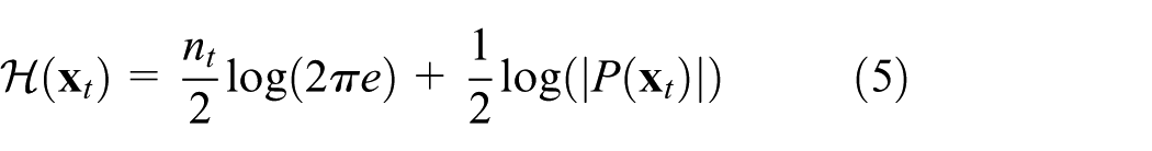
The goal of sensor network planning problems is to find out the optimal sensing locations that maximize the information reward about the target states. Here, the information reward can be thought of as a reduction in the uncertainty of the variable of interest due to the information included in the measurement variables. This uncertainty reduction is quantified with mutual information, which is the difference between the prior and posterior entropy of

where


where

Since a sensor network has limited resources, the system should select the set of sensing points that give the maximum information about the target states to reduce the number of observations. Therefore, a sensor network planning problem can be stated as selecting the most informative set of sensing points

Note that ith sensing location
Sensor network planning as a potential game
Potential games are applied to many engineering optimization problems (such as cooperative control 21 and resource allocation 22 ) due to their static (existence of Nash equilibrium) and dynamic properties (simple learning algorithm). 17 This section provides the required game-theoretic background used to develop the results in this article and describes a potential game formulation of a sensor network planning problem. Finally, we present limitations in applying the approach to a large sensor network.
Game-theoretic architecture
Consider a finite game in strategic form consisting of three components: 23
A finite set of players (agents):
Strategy spaces: a finite set of actions (strategies)
Utility functions: a utility (payoff) function
Accordingly, a finite strategic-form game instance is represented by the tuple
A utility function

for every
A potential game is a non-cooperative game in which the incentive of the players changing their actions can be expressed by a single function, called the potential function. That is, that the player tries to maximize its utility is equivalent to maximizing the global objective for a set of all the players. 24
Definition 1
A finite non-cooperative game

for every
The property of a potential game in equation (9) is called a perfect alignment between the potential function and the player’s local utility functions. In other words, if a player changes its action unilaterally, the amount of change in its utility is equal to the change in the potential function.
Potential games have two important properties. 17 The first one is that the existence of pure strategy Nash equilibrium is guaranteed. Since in a potential game the joint strategy space is finite, there always exists at least one maximum value of the potential function. This strategy profile maximizing the potential function locally or globally is a pure Nash equilibrium. Hence, every potential game possesses at least one pure Nash equilibrium. The second important property is the presence of well-established learning algorithms to find a Nash equilibrium by repeating a game. Many learning algorithms for potential games are proven to have guaranteed asymptotic convergence to a Nash equilibrium. 21
In this article, our main focus is to approximate utility functions of a potential game. To address strategy profiles in a near potential game with approximate local utility functions, a near Nash equilibrium is introduced. A strategy profile

for every
Cooperative sensing as a potential game
From a game-theoretic perspective, each sensing agent is considered a player in a game who tries to maximize its own local utility function,

The local utility function can be represented by

With this local utility function, the designed potential game is solved by repeating the game for
Learning Algorithm

The learning algorithms are varied according to a specific update rule

In Marden et al.,
12
it is shown that the expected utilities

Having computed
Computational complexity analysis
As described in Choi and How, 6 the potential game-based approach to cooperative sensor planning enables one to find out the informative set of sensing locations with much less computation than an exhaustive search. However, a conditional mutual information conditioned on the other agents’ sensing locations has limitations when applied to a large sensor network, because every agent needs information about the decisions made by the other agents in the previous stage. If the communication network is strongly connected, one agent’s decision can be forwarded to all the other agents, and then the next stage can be initiated after this information exchange has happened. This decision sharing among all the agents incurs substantial communication cost/traffic. In addition to this communicational burden on a network, the conditional mutual information itself increases computation load on each agent’s processing unit for obtaining utility values. In this section, we will analyze the computational complexity for JSFP algorithm applied to sensor network planning in more detail.
As shown in Algorithm 1, the distributed solution of a potential game is obtained by repeating a one-shot game until it converges to equilibrium. In JSFP, at each stage

where
The main reason for the computation load of
where
Approximate local utility design
In this section, an approximation method is proposed to reduce the computational and communicational burden of computing the local utility function. The method modifies the form of a local utility function itself by removing some of the conditioning variables, which represent the decisions of other agents.
Approximate utility function
The proposed approximation method for computing the local utility function is to reduce a number of the conditioning variables using the correlation structure of the information space, making the local utility function depend on the part of the decisions
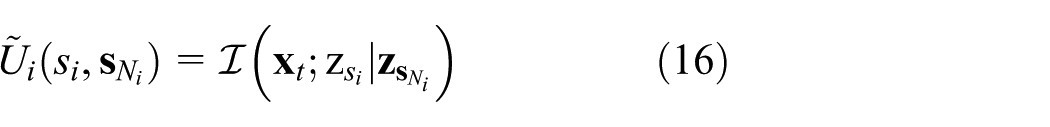
where
Lemma 1
Let

where
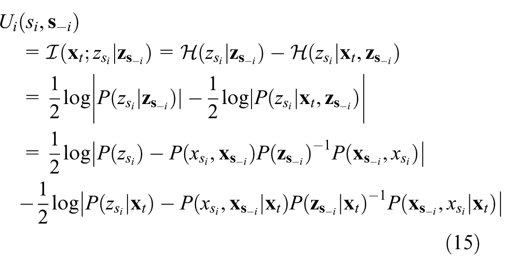
Proof
The conditional mutual information of equations (12) and (16) can be expanded using chain rule 20

Canceling out common terms results in the first equation (17a). To obtain the second equation (17b), a preliminary result is given for exchanging of conditioning variables in mutual information 3

Equation (17b) follows by rewriting the third term of equation (18) using the above property

Remark 1
In a target tracking example, the difference (equation (17b)) between the approximate local utility and the true local utility can be simplified as

Applying the assumption that the measurements are conditionally independent given the target states, the last term in equation (17b) becomes zero, then the error can be represented with mutual information between the sensing selections related with sensing agent
Remark 2
In cooperative games, the common terms
To keep the error incurred by the approximation small, we propose two neighbor selection algorithms: geometry-based and correlation-based. These methods differ in the definition of the distance between sensing points. In geometry-based selection, the distance between two sensing points is the spatial distance as the name suggests. It can be obtained simply by calculating the Euclidean distance between the sensing locations. On the other hand, the correlation-based method uses the correlation between measurement variables taken at the sensing points as a measure of closeness. In most cases, the geometric closeness of the sensing points can be translated into correlation between the measurements taken at those locations. That is, the more closely located sensors are, the more correlated their measurements. Therefore, the geometry-based approach is sufficient for neighbor selection in many applications. However, when the target states exhibit highly nonlinear spatiotemporal dynamics, the closeness in sensing locations has nothing to do with the correlation between the corresponding measurements. Thus, we propose the correlation-based selection algorithm to address this nonlinearity issue.
Geometry-based neighbor selection algorithm
Intuitively, the simplest way to determine the neighbor set for each agent is by defining the neighborhood by closeness in geometric distance. In many cases, such as monitoring spatial phenomena as in Krause et al., 4 geometric closeness of two sensing locations can be translated into correlation between corresponding measurement variables taken at those locations. In this section, we propose a selection algorithm in which neighbors are selected as agents located within some range from each agent. We refer to this selection method a geometry-based neighbor selection.
One technical assumption made in this section is that the communication network can be represented as a connected undirected graph,

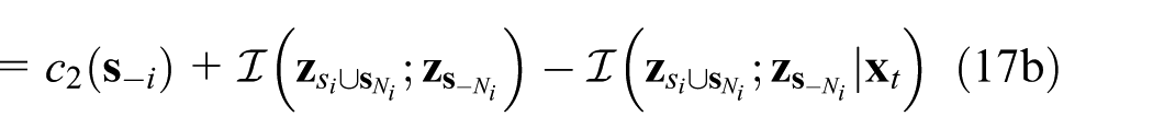
From equation (19), a game defined by the local utility in equation (16) is not necessarily a potential game with potential function in equation (11), because the last bracket termed difference in potentiality does not vanish in general. (This statement does not exclude possibility of a potential game with the same local utility function for a different potential function.) Instead, further analysis can be done to identify the condition under which this localized version of the game constitutes a potential game aligned with the objective function of the cooperative sensing.
The last term in equation (19) can also be represented as
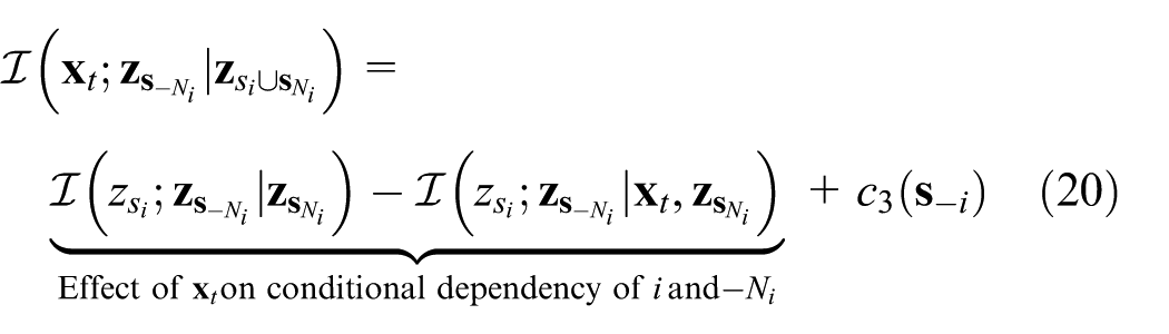
by using equation (16). Noting that the last term in equation (20) does not depend on agent i’s action, the difference in potentiality represents how significantly the verification variable
Proposition 1
If

for any
Proof
Proof is straightforward by noting that
In other words, if
Proposition 2
If there exists
constitutes a potential game with global potential (equation (11)).
There are some contexts that the conditional independence condition is at least approximately satisfied. Many physical phenomena are associated with some notion of time and length scale. If the correlation length scale of the motion of interest is order of inter-agent distance, there will be no too significant dependency between agents far from each other; then, the conditional independence assumption in the previous propositions can be satisfied. This statement certainly is domain and problem dependent; it is not appropriate to make some general statement of satisfaction of the conditional independence assumption.
Correlation-based neighbor selection algorithm
As shown in equation (17), the error incurred by the approximation of the local utility function can be considered in two ways. In the first equation, the error is the mutual information between the target states and the measurement variables which is not in the neighbor set of agent
For the second way, the error can be considered as the difference between the prior mutual information and the posterior mutual information conditioning on the target states. This amounts to the mutual information of the variables at
To make the error sufficiently small, the method to select the neighbor set for each agent should be determined. In most cases, measurement variables taken at close locations are correlated with each other, and measurements taken at distant locations from sensing agent i’s search space have little correlation with agent i’s selection. Thus, each sensing agent can approximate its utility function by considering the neighbor set consisting of sensing agents close to each agent. However, for example, in sensor planning for weather forecasting, the assumption that closeness in Euclidean distance means correlation between variables is broken. Weather dynamics is highly nonlinear, and thus, the neighbor set should be chosen in different ways from usual cases. For nonlinear target dynamics, such as a weather forecast example, a sequential greedy scheme is proposed. Every sensing agent conducts the greedy scheme to determine its neighbor set. The algorithm simply adds sensing agents in sequence, choosing the next sensor which has maximum mutual information about the target states conditioned on the measurement variables of a sensing agent’s search space and its pre-selected neighbors. Using the first error bound in equation (17), the algorithm greedily selects the next sensing agent

Algorithm 2 shows the greedy neighbor selection algorithm.
Neighbor Selection Algorithm for Weather Forecast Example

If we leave out measurement variables that have little correlation with the selection of sensor
Analysis of approximate potential game
The approximate utility functions cause a change in the preference structure of the players and break the alignment condition for a potential game. It follows that the game cannot guarantee the existence of a pure Nash equilibrium which exists in the potential game with the true utility function. However, if the approximation error in a utility function stays small, we can expect that a game with the approximate utility functions has similar properties to that of the potential game. 29 Before presenting the theorem for the equilibria of two games that are close in terms of payoffs, we first introduce the following lemma from Candogan et al. 17
Lemma 2
Consider two games
The difference between
Definition 2
The MPD between two games
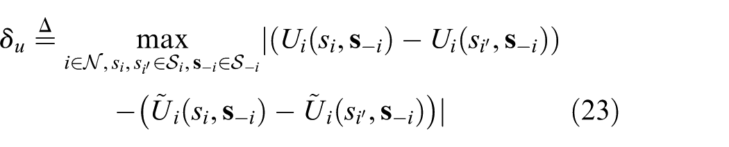
The MPD represents the distance between two games in terms of the difference of unilateral utility changes rather than the difference of their utility values. This notion of distance between games identifies a strategic equivalence between them.
29
This is because, as mentioned in Remark 2, the preference structure is determined by the amount of the utility improvement due to unilateral deviations of each agent

This result comes from the proof of Lemma 3. Let
In case
Theorem 1
Consider a potential game
Proof
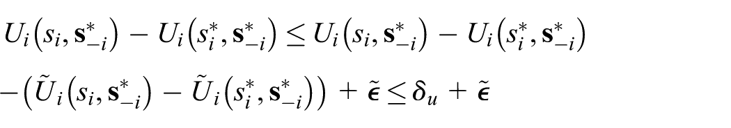
Since a Nash equilibrium is an
This result implies that the Nash equilibria of a potential game with the true utility function are included in the approximate equilibria of the game with approximate utility functions. That is, if we let the set of

for every
Corollary 1
Consider a potential game

for every
Proof

there exists at least one Nash equilibrium in
We have demonstrated the existence of equilibrium points in the games with approximate utility functions, but there remains an issue about efficiency of the resulting equilibrium points. Candogan et al. 29 provided a learning dynamics for a near potential game and showed that convergence to a small neighborhood of the equilibria from the original game can be established. However, we still have an efficiency issue of the equilibria. For a potential game, log-linear learning is shown that it guarantees on the percentage of time that the strategy profile will be at a potential maximizer. 30 However, it is not known how quickly this learning dynamics converges to the best solution. In Choi and Lee, 1 we demonstrated the validity and efficiency of the JSFP method through numerical examples. Likewise, we will show the efficiency of the resulting equilibrium with numerical simulations.
Numerical examples
The proposed approximation method is demonstrated on two numerical examples with nonlinear models: sensor management for multi-target tracking and sensing point targeting for weather forecast. In the first example, we apply the localized utility function to a sensor selection problem for multi-target tracking. In target tracking, the sensors gain information about the kinematic state of a group of target and the measurement model is generally nonlinear, such as the range to the target or bearing only measuring Infrared (IR) sensors. A particle filter has been successfully applied to estimating the target states with better performance than Kalman filters. However, computation of mutual information for a particle filter grows exponentially with the number of sensing points; thus, it is impossible to calculate entropy with full information. The first example shows that the approximation method enables a potential game approach to be applied to a sensor planning problem with a large sensor network. Also it demonstrates the efficiency of the geometry-based neighbor selection algorithm, because the geometric distance between sensing points is related with the amount of information about the target states. The other example is sensor targeting in the context of numerical weather forecast. While the first example shows the performance of the approximation local utility itself and the simple neighbor selection method is sufficient to limit the conditioning variables, the weather forecast example allows comparison of two neighbor selection algorithms: a geometry-based method and a correlation-based method. Since the weather dynamics is highly nonlinear, the closeness in sensing locations has nothing to do with the correlation between the corresponding measurements.
Multi-target tracking
To demonstrate performance of the proposed game-theoretic approach under a nonlinear and non-Gaussian sensor model, a multi-target tracking example is investigated. A similar example using the JMPD technique introduced in Kreucher et al. 31 has been referred.
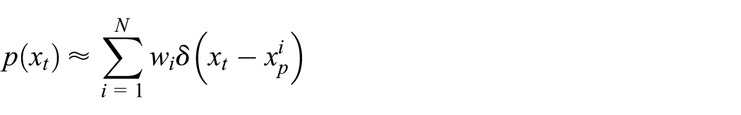
JMPD is a specialized particle filter method which helps estimate the number of multi-targets and state of each target effectively. JMPD approximates the multi-target state with

where
In this example, a fixed sensor network tries to estimate the number and states of multi-targets moving within a 2400 m × 2400 m region with nearly constant speed. In this space, image sensors are uniformly arranged to detect targets. Each sensor gives detection (1) or non-detection (0) as a measurement value according to the range-based detection rate as follows

where
The objective of this sensor problem for the multi-target tracking is finding a set of sensing points maximizing the mutual information about the multi-target states at a given situation. Similarly, as in the next weather forecasting example, each agent needs to evaluate the local utility to obtain a cooperative solution. The local utility and its approximate version can be evaluated by using equations (12) and (16), respectively. Mutual information under a particle filter framework can be computed using the Monte Carlo integration technique below (see Hoffmann and Tomlin 3 for more detailed derivation). Here, the computation of the integral is equivalent to a finite sum since the possible measurement is only 0 or 1

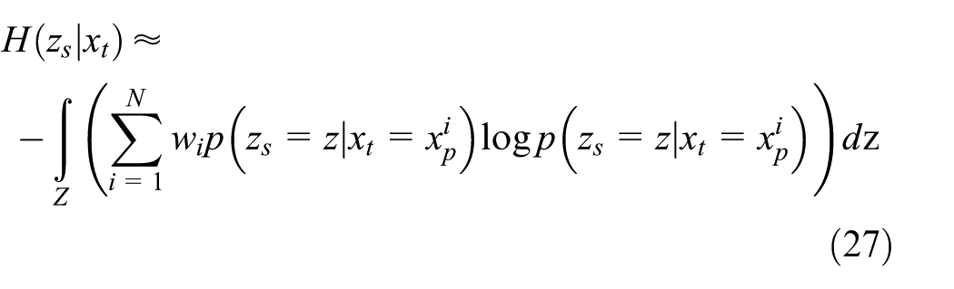
Note the variables in the equation; local utility each agent evaluates cannot coincide with each other if each agent does not share the same particles. Especially in a situation when agents have poor information about the multi-target, it is highly probable that each agent will have different particle sets. Then each agent will estimate different values of the utility even with the same observation result, interrupting cooperation among sensor networks. However, this problem can be solved easily by assuming that agents have the same random generator and share the same random seed so that they can generate exactly the same pseudorandom numbers.
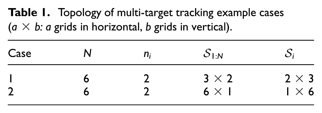
The proposed game-theoretic method has been tested for two different sensing topologies: six sensors in a 3 × 2 grid and six sensors in a 6 × 1 grid, where each grid corresponds to a 400 m × 400 m region over a 2400 m × 2400 m space, as described in Table 1. Each sensor is located in the center of its grid. A sensor can select maximum

Topology of multi-target tracking example cases (a × b: a grids in horizontal, b grids in vertical).
As a simulation scenario, a two-target scenario after one observation with each JMPD step is considered. A detailed situation is described in Figure 2. As shown in the figure, sensors estimate the multi-target states under high uncertainty; thus, proper choice of sensing points becomes important to obtain a large amount of information using the same sensor resources.

Scenario and sensing points determined by the correlation-based approximate JSFP in each case. Red stars: true positions of multi-targets. Green dots: particles estimating the state of multi-target.
The proposed method is compared with greedy strategies and the JSFP algorithm with full information. The global optimum solution is not evaluated since it is hardly obtained in tractable time under the particle filter framework. Instead, full information JSFP algorithm has been assumed to give a near optimal solution. The compared approaches are (1) greedy strategies in which each agent makes a locally optimal decision using partial information, (2) JSFP learning algorithms in which a local utility is obtained using full information about the other agents’ decisions, and (3) JSFP learning rule in which a local utility function is approximated by limiting conditioning variables to the neighbor’s decisions. Neighbors are defined in two different ways. One is determined in terms of multi-hop in communication and the other defines neighborhood with correlation in search space. These distributed methods are presented in detail as follows:
Local greedy: Local greedy strategy maximizes the mutual information of its own selection as shown below

Sequential greedy: Each agent selects the sensing location, which gives the maximum mutual information conditioned on the preceding agents’ decisions

JSFP with inertia: Implementation of Algorithm 1 with inertia, that is, an agent is reluctant to change its action to a better one with some probability (in this example, with probability
JSFP without inertia: Implementation of Algorithm 1 without inertia.
Approximate JSFP with two-hop neighborhood with inertia: Iterative process with local utility functions defined in equation (16). In this strategy, the neighbors are determined in terms of multi-hop in inter-agent communication—that is, by the geometry-based selection algorithm.
Approximate JSFP with correlation-based neighborhood with inertia: Iterative process with local utility functions defined in equation (16). The neighbors are determined by Algorithm 2 using the correlation structure of the search space.
The resulting objective values for six different strategies are given in Table 2, and the histories of objective values in the iterative procedure are shown in Figure 3.
Objective values for six different strategies.

JSFP: joint strategy fictitious play.

Histories of objective values with stage count for two cases.
Primarily, the JSFP with full information gives the best solution compared to other strategies as expected. In addition, the approximate JSFP gives a better solution than greedy strategies. As seen in case 1, approximate JSFP gives the same solution as JSFP with full information. However, unlike in the weather forecasting example, the correlation-based approximate JSFP does not always show better performance than the geometry-based approximate JSFP. The first reason is that there is no complex correlation between the sensors, and the correlation is highly related to the Euclidian distance. Second, approximate JSFP algorithms sometimes exhibit an interesting feature in that it may meet the optimal solution during its iteration but does not adopt it, as shown in the correlation-based approximate JSFP of the second example. This is because local utility approximation breaks the potentiality, and agreement among sensors no longer guarantees cooperation. Most importantly, the approximate JSFP algorithm can reduce the computational burden of the JSFP algorithm efficiently while still obtaining a good cooperative solution. Note that calculating the local utility through equations (26) and (27) incurs proportional costs to
Sensor targeting for weather forecast
The proposed game-theoretic method is demonstrated on a sensor targeting example for weather forecast using Lorenz-95 model. The Lorenz-95 model 32 is an idealized chaos model that is implemented for the initial verification of numerical weather prediction. In this article, we consider a sensor targeting scenario as Choi and How 6 in which a two-dimensional (2D) extension of the original one-dimensional (1D) Lorenz-95 model was developed and adopted. The 2D model represents the global weather dynamics of the mid-latitude region of the northern hemisphere as follows 1

where
The sensor targeting problem for the weather forecast can be rephrased as selecting the optimal sensing locations in the search region at

where the measurement equation is given by
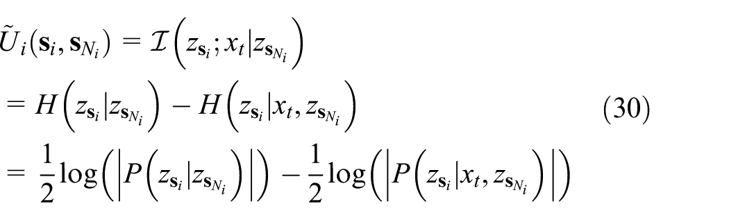
In a potential game, each agent computes the local utility function defined by the conditional mutual information between the measurement selection and the verification variables conditioned on the other agents’ action. We obtain the local utility using the backward scheme as the mutual information of the global objective as in equation (15). We should calculate the two matrices
The approximate local utility is computed in the same way as computing the local utility (equation (15)) with the exception of the conditioning variables. The conditioning variables are replaced with the neighboring agents instead of all the other agents’ selections
The proposed game-theoretic method using an approximation of the local utility has been tested for three different sensing topologies; 9 sensors in a 3 × 2 format in two different search spaces and 15 sensors in a 2 × 3 format in a larger region than the first and second cases, as described in Table 3. An oceanic region of size 12 × 9 (in longitude × latitude) is considered as a potential search region, among which the whole search space
Topology of example cases (a × b: a grids in longitude, b grids in latitude).

The resulting objective values for the seven different strategies are given in Table 4, and the histories of objective values in the iterative procedure are shown in Figure 4. The results for iterative algorithms with inertia are obtained from Monte Carlo simulation and represent average objective values. Case 3 is different from the other two cases in that a larger sensor network is considered, and the global optimal solution cannot be obtained in tractable time. However, from the examples of small sensor networks, we consider that the optimal solution of the third case may be close to the JSFP with full information. Thus, we can consider the objective value for the JSFP with full information as an upper bound for the sensor networks with a large number of sensors.
Objective values for seven different strategies.

JSFP: joint strategy fictitious play.
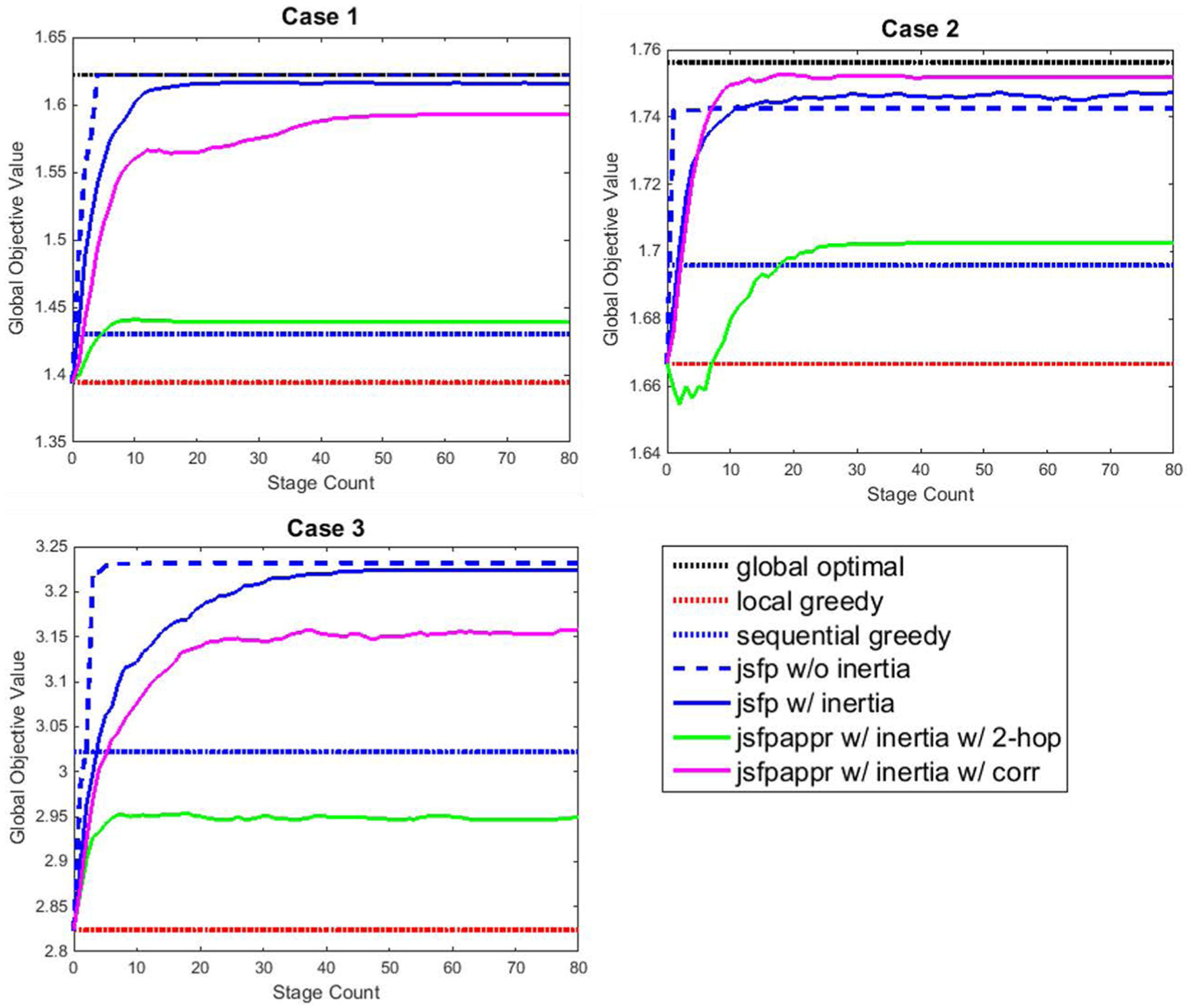
Histories of objective values with stage count for three cases.
First, note that the JSFP with full information of other agents’ actions gives a better solution than the sequential greedy algorithm, and the solution is the same as or close to the optimal solution in Choi and Lee. 1 The sequential greedy strategy can be considered as a baseline for comparing the performance of different strategies, since it guarantees the worst-case performance in polynomial time, even though the guarantee is applied to problems in which the objective functions satisfy some conditions. The JSFP with approximate local utility functions also presents a better performance than the sequential greedy strategy except for approximate JSFP with two-hop neighborhood of the third example. The approximate local utility function based on the correlation always gives a better solution than ones depending on the actions of the neighbors selected by geometry-based method. In cases 1 and 2, the objective value for the approximate JSFP with a correlation-based neighborhood is close to the JSFP with full information. The important thing to note here is that the number of conditioning variables used for computing the utility functions is half of the JSFP with full information. As mentioned in the “Computational complexity analysis” section, the computation time for the conditional mutual information increases proportional to the cubic of the conditioning variables. Therefore, the computation time for the approximate local utility function is reduced by a factor of approximately 8.
Conclusion
An approximation method for computing the local utility function has been presented when a sensor network planning problem is formulated as a potential game. A local utility function of each agent that depends on the neighboring agents’ decisions is presented, and a neighbor selection algorithm is proposed to keep the error induced by the approximation small. Two sensor targeting examples for weather forecasting and multi-target tracking demonstrated that potential game formulation with the approximation local utility function gives good performance close to a potential game with full information.
Footnotes
Handling Editor: Konstantinos Kalpakis
Declaration of conflicting interests
The author(s) declared no potential conflicts of interest with respect to the research, authorship, and/or publication of this article.
Funding
The author(s) disclosed receipt of the following financial support for the research, authorship, and/or publication of this article: This work was supported in part by Agency for Defense Development under contract #UD140053JD and in part by Air Force Office of Scientific Research (AFOSR) grant (FA2386-16-1-4064) via Asian Office of Aerospace Research and Development (AOARD).