Minimum-latency data aggregation scheduling based on multi-path routing structures under physical interference model

Abstract

Minimum-Latency Aggregation Scheduling is a significant problem in wireless sensor networks. The key challenge is to find an effective solution to aggregate data from all sensors to the sink with minimum aggregation latency. In this article, we propose a novel data aggregation scheduling algorithm under the physical interference model. First, the algorithm partitions the network into square cells according to the communication range of a sensor. Second, a node is selected randomly as the aggregated node to receive the data from the other nodes in the same cell. Finally, a data aggregation tree, which consists of multiple disjoint paths, is constructed to aggregate data from all aggregated nodes to the sink. We empirically proved that the delay of the aggregation schedule generated by our algorithm is (K+1)²Δ−K−1+2λ time-slots at most, where K is a constant depending on the sensors transmitting power, the signal-to-interference-plus-noise-ratio threshold, and the path-loss exponent; $\mathrm{\Delta }$ represents the maximal number of nodes in a cell; and $\lambda$ denotes the number of cells at a row/column in a square network area. Simulation results also show that our algorithm achieves lower average latency than the previous works.

Introduction

Data aggregation^1,2 is an important technique in wireless sensor networks (WSNs), which is the combination of data coming from different sensors according to a certain aggregation function (e.g. maximum, minimum, or/and average values of all data), and eliminates unnecessary packet transmission by filtering out redundant sensor data. However, data aggregation will increase the transmission latency because data cannot be sent immediately until all data are aggregated by a sensor. ³ On the contrary, collision will occur when two or more sensors send data simultaneously to their common neighbor. Once the collision occurs, the sensor has to spend more time retransmitting data. ⁴ Therefore, for some delay sensitive applications such as intruder detection, medical care, fire monitoring, and battle field monitoring in WSNs, it is essential to adopt an effective data aggregation schedule method to transmit data from sensors to the sink as fast as possible.

Currently, many researchers have investigated the Minimum-Latency Aggregation Scheduling (MLAS) problem. For example, most existing research works^5–13 studied the MLAS problem under the protocol interference model and bound the aggregation latency of $O(\mathrm{\Delta }+R)$ , where $R$ is the network radius and $\mathrm{\Delta }$ is the maximum node degree. However, the protocol interference model does not accurately reflect wireless interference in reality. In contrast, the physical interference model ¹⁴ is more realistic and captures the cumulative interference between links more accurately. Due to the challenge of handling the cumulative interference effect, only a few previous works^15–22 studied the MLAS problem under the physical interference model.

In this article, we continue to explore the MLAS problem under the physical interference model with the same transmission power. We design a novel data aggregation scheduling algorithm, which is called Data Aggregation Scheduling based on Multi-Path Routing Structures (DAS-MPRS) algorithm. The algorithm partitions first the network into square cells according to the sensor’s communication range. Then, an aggregated node is selected randomly in each cell so as to receive data from other nodes in the same cell. Finally, a data aggregation tree is constructed by using multiple disjoint paths to connect the aggregated nodes. The aggregated data are transmitted one by one along these disjoint paths. The main contributions are summarized as follows:

1. The time of constructing a data aggregation tree by DAS-MPRS algorithm is less than that of the existing algorithms. In general, the existing algorithms^15–17 establish an aggregation tree based on the connected dominating set (CDS) or maximal independent set (MIS). It has to spend additional time seeking out an MIS and some connectors to form a data aggregation tree. However, our algorithm selects randomly a node in each cell and a data aggregation tree is formed by using multiple disjoint paths to connect these nodes. Especially, when a node or a link fails during the data aggregation, the existing algorithms have to spend more time reconstructing an aggregation tree. Nevertheless, DAS-MPRS algorithm will take less time to reconstruct an aggregation tree by selecting randomly a new node to replace the failure node in the same cell.

2. The latency bounds of DAS-MPRS algorithm is $(K+1{)}^2\mathrm{\Delta }-K-1+2\lambda$ , where $K$ is a constant depending on the sensors transmitting power, the signal-to-interference-plus-noise-ratio (SINR) threshold, and the path-loss exponent; $\mathrm{\Delta }$ is the maximal number of nodes in a cell; and $\lambda$ denotes the number of cells at a row/column in a square network area. Currently, the best result ¹⁷ for the MLAS problem is bounded by $(K+3{)}^2(\mathrm{\Delta }+2R)+R$ , as far as we know. Simulation results show that our algorithm achieves lower average latency than the previous works.

The remainder of this article is organized as follows. The “Related works” section summarizes the relevant work and the section “System model and problem statement” formulates the problem of MLAS. A detailed description of DAS-MPRS algorithm is given in the section “Algorithm design” and the performance analysis of the algorithm is presented in the section “Algorithm analysis and performance evaluation.” The final section concludes the main findings.

Related works

The MLAS problem has been proved to be non-deterministic polynomial (NP)-hard under the protocol interference model. ⁵ Chen et al. ⁵ designed an approximate algorithm with a latency bound of $(\mathrm{\Delta }-1)R$ , where $R$ is the network radius and $\mathrm{\Delta }$ is the maximum node degree. Subsequently, Zhu and Hu ⁶ propose a new approximate algorithm with the performance ratio of $(7\theta /(\underset{2}{\log }|S))+c$ , where $S$ is the set of sensors containing source data, $\theta$ is the maximal number of sensors within the transmission range of any sensor, and $c$ is a constant. Constructing a data aggregation tree based on MIS, Huang et al. ⁷ raised a new approximation algorithm whose latency bound is $23R+\mathrm{\Delta }-18$ . However, Yu et al. ⁸ discovered that a collision-free schedule cannot be derived in some cases. Hence, they put forward a distributed algorithm which has latency of $24D+6\mathrm{\Delta }+16$ , where $D(R\le D\le 2R)$ is the network diameter. Unfortunately, the upper bound of Yu et al.’s algorithm ⁸ is worse than that of Huang et al.’s algorithm. ⁷ Realizing the disadvantage of these algorithms, Wan et al., ⁹ Ren et al., ¹⁰ and Xu et al. ¹¹ proposed some improved approximate algorithms whose latency is bounded by $15R+\mathrm{\Delta }-4$ , $15R+\mathrm{\Delta }-15$ , and $16R+\mathrm{\Delta }-14$ , respectively. Considering the common neighboring dominators, Nguyen et al. ¹² made further improvement for the above works, and designed a new collision-free scheduling algorithm which has the latency of $12R+\mathrm{\Delta }-11$ . Recently, Guo et al. ¹³ designed a distributed scheduling algorithm based on a novel cluster-based aggregation tree, which has a latency bound of $4R\prime +2\mathrm{\Delta }-2$ , where $\mathrm{\Delta }$ is the maximum degree and $R\prime$ is the inferior network radius.

Although the protocol interference model has been used in many studies, it ignores cumulative interference caused by the other concurrently transmitting nodes. Moscibroda et al. ²³ demonstrated experimentally that real-world phenomena cannot be captured adequately under the protocol interference model. Thus, researchers moved to investigate the MLAS problems under the physical interference model proposed by Gupta and Kumar. ¹⁴ Under this interference model, whether a packet is received successfully by the receiver depends on the received signal strength, the background noise level, and the cumulative interference caused by simultaneously transmitting nodes. Compared with the protocol interference model, the physical interference model can capture the cumulative interference more accurately in the real wireless environment. Li et al. ¹⁵ designed a scheduling algorithm whose latency is bounded by $K^2(62R+\mathrm{\Delta })+R$ exploiting the uniform power scheme, where R is the network radius, $\mathrm{\Delta }$ is the maximum node degree and, K is a model-specific constant depending on the sensor node’s transmitting power, the SINR threshold, the path-loss exponent, and so on. Thereafter, Xu et al. ¹⁶ proposed an improved approximation algorithm with a latency bound of $6(K+1{)}^2(\mathrm{\Delta }+2R+O(\log R))$ . Recently, Xu et al. ¹⁷ designed a new data aggregation scheduling algorithm whose latency is bounded by $(K+3{)}^2(\mathrm{\Delta }+2R)+R$ , which has the best result for the MLAS problem under the physical interference model, as far as our awareness is concerned. In addition, An et al. ¹⁸ made the milestone contribution to prove the NP-completeness of the MLAS problem under the physical interference model. Subsequently, Lam et al. ¹⁹ demonstrated that MLAS problem is the approximable (APX)-hardness in the metric SINR model without power control.

In addition, researchers studied the same problem with power control, that is, the node’s transmission power is unlimited. Wang and Baras ²⁰ designed a distributed algorithm achieving the time-latency bound of $O(\Lambda )$ , where $\Lambda$ is the logarithm of the ratio between the lengths of longest and shortest links in the network. Later, Lam et al. ²¹ proposed an approximate algorithm using $O(R+\Lambda )$ time-slots at most to complete the aggregation task, where $R$ is the network radius. Recently, Li et al. ²² presented a distributed algorithm whose latency is bounded by $O(\Lambda )$ and a centralized algorithm with a latency bounded by $O(\stackrel{3}{\log }n)$ , where $n$ is the number of nodes.

System model and problem statement

Network model

Assume that a WSN consists of a number of sensor nodes, which has the same transmission power, and the sink, which is responsible for gathering data from all sensor nodes. All the nodes are distributed randomly in the Euclidean plane. Any node cannot send and receive simultaneously. Under the physical interference model, a node $v$ , which receives a data packet from a node $u$ , may be interfered by other nodes which send data concurrently. Therefore, a receiver $v$ successfully receives a message from its sender $u$ if and only if it satisfies the following condition

$$SIN{R}_v=\frac{\frac{P_u}{d{\left(u,v\right)}^{\alpha }}}{N_0+{\displaystyle \sum _{w\in S-u}\frac{P_w}{d{\left(w,v\right)}^{\alpha }}}}\ge \beta$$

(1)

where $P_u$ denotes node u’s transmission power, $d(u,v)$ is the Euclidean distance between node $u$ and node $v$ , $N_0$ is ambient noise, $\alpha \in (2,6)$ ^17,22 denotes the path-loss exponent, $\beta \ge 1$ is the minimum SINR required for a message to be successfully received, and $S$ is the set of concurrently transmitting nodes, which are scheduled in the same time-slot.

According to equation (1), a node u can communicate with a node v if and only if their communication distance $\ell (u,v)\le r_{\max }=(P/N_0\beta {)}^{1/\alpha }$ . Obviously, if the communication distance $\ell (u,v)$ is comparatively close to $r_{\max }$ , it will reduce the number of simultaneous transmitting nodes due to communication interference. For instance, when the communication link $\ell (u,v)=r_{\max }$ , a packet is transmitted successfully from node u to node v if and only if there is no other simultaneous transmission. Hence, we set the node’s transmission radius $\mathbf{r}=\delta ·r_{\max }$ , where $\delta \in (0.1,0.9)$ is a constant which is considered by Li et al. ¹⁵ and Xu et al. ¹⁷ Thus, a WSN can be modeled as an undirected graph $G=(V,E,\mathbf{r})$ , where V is the set of nodes, $v_s$ $\in V$ represents the sink, and an edge $e=(u,v)\in E$ exists if the communication distance $\ell (u,v)\le \mathbf{r}$ .

Problem statement

Assume that time is divided into equal-sized slots normalized to one and each node is assigned a time-slot to transmit data. The problem is to design a feasible scheduling sequence $S=\{S_1,S_2,\dots ,S_T\}$ , where $T$ is the length of schedule or the schedule latency, $S_t\subset V$ denotes the set of nodes being scheduled at time-slot $t(t\in \{1,2,\dots ,T\})$ . A correct aggregation schedule sequence must satisfy the following conditions:

1. Any sensor node should be scheduled exactly once, that is, $S_i\cap S_j=\varphi$ , $i\ne j$ ;

2. A node cannot act as a transmitter and a receiver in the same time-slot;

3. For each time-slot $t$ , node u’s $(u\in S_t)$ data should be successfully received by the corresponding receiver node $v$ , that is, $\mathrm{SIN}{R}_v\ge \beta$ ;

4. Data are aggregated from $S_k$ to $V-\bigcup _{i=1}^k{S}_i$ at time-slot k, for all $k=1,2,\dots ,T$ , and all the data are aggregated to the sink $v_s$ at $T$ time-slots, that is, $\bigcup _{i=1}^T{S}_i-v_s$ .

The MLAS problem studied in this article can be formally defined as follows: Given a WSN that consists of a number of sensors and the sink, and their locations, supposing each sensor has a piece of data to be transmitted to the sink, the goal is to design a valid aggregation schedule $S$ satisfying the above four conditions and minimize the total number of schedule latency.

Algorithm design

In this section, we present a novel data aggregation scheduling algorithm, which is called DAS-MPRS algorithm, to minimize the schedule latency. The algorithm has two main phases: constructing an aggregation tree and scheduling data from all sensors to the sink. In the first phase, the plane is partitioned into small square cells with the same edge length. Then, a node is selected randomly to act as an aggregated node in each cell. Finally, an aggregation tree is constructed by using multiple disjoint paths to connect the aggregated nodes located at the cells with the same column or row. With regard to each cell, an edge is created from an ordinary node to the aggregated node. In the second phase, the data are collected first by the aggregated node in each cell. Then, the aggregated data are transmitted from the aggregated nodes to the sink according to the aggregation tree.

Network partition

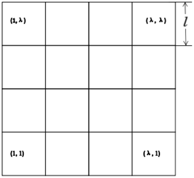
Given that the whole network is distributed in a square region with side length $L$ , we partition the network into small square cells with edge length $\ell =\mathbf{r}/\sqrt{5}$ , by a group of horizontal and vertical lines. In order for the sensors in a cell to transmit their data to the sensors in the neighboring cells (sharing a common side), we set $r=\delta ·r_{\max }$ , which is mentioned in the section “Network model.” The divided network is shown in Figure 1. Let $\lambda =\lceil L/\ell \rceil$ denote the number of cells in a row or column, we assign each cell positive integer coordinates (i, j) $(1\le i,j\le \lambda )$ , and a cell with coordinates (i, j) is denoted by cell ${\gamma }_{i,j}$ . Accordingly, the bottom-left corner cell is denoted by ${\gamma }_{1,1}$ and the upper-right corner cell is called ${\gamma }_{\lambda ,\lambda }$ .

Figure 1.

Network partition.

Construction of a data aggregation tree

After partitioning the network into many small square cells, we select randomly a node as the aggregated node in each cell. Let $v_{i,j}$ denote the aggregated node in the cell ${\gamma }_{i,j}$ , and we also assume that the sink $v_s$ is denoted by $v_{x,y}$ . That is to say, the sink may be located at the cell ${\gamma }_{x,y}$ . For convenience of description, an aggregated node is called a supernode if it has the same row with $v_{x,y}$ , denoted by $v_{x,j}(j\ne y)$ .

A data aggregation tree is constructed according to the following rules:

1. For each node $v$ in cell ${\gamma }_{i,j}$ , a directed link is created from $v$ to $v_{i,j}$ .

2. For the aggregated node $v_{i,j}$ , a directed link is formed from $v_{i,j}$ to $v_{i+1,j}$ if $i<x$ . Otherwise, a directed link is created from $v_{i,j}$ to $v_{i-1,j}$ .

3. Similarly, for every supernode, a directed edge is created from $v_{x,j}$ to $v_{x,j+1}$ if $j<y$ . Otherwise, a directed edge is created from $v_{x,j}$ to $v_{x,j-1}$ .

The construction process of a data aggregation tree is shown in Figure 2. In order to optimize description of the data aggregation scheduling in the following section, we introduce two concepts as follows.

1. Primary path. A primary path is the path which connects the aggregated nodes with the same row and its endings is a supernode.

2. Backbone path. A backbone path is the path connecting the supernodes and its endings is the sink.

Figure 2.

Construction of a data aggregation tree.

For instance, there are 16 primary paths and 2 backbone paths in Figure 2.

Data aggregation scheduling

In this section, we describe more details of the DAS-MPRS algorithm (see Algorithm 1). To describe conveniently, assume that the sink $v_s$ is located at the top-right corner cell ${\gamma }_{\lambda ,\lambda }$ . Note that when the sink is located at any position of the network, we can achieve the same results by making a little modification of our algorithm.

Algorithm 1 DAS-MPRS algorithm

1: Partition the deployment plane into square cells with side length $\ell =\mathbf{r}/\sqrt{5}$ ; 2: Select randomly a node to act as an aggregated node $v_{i,j}$ in the cell ${\gamma }_{i,j}$ ; 3: Set $K=\lceil (4P\beta \tau {\ell }^{-\alpha }/(5^{(-\alpha /2)}P{\ell }^{-\alpha }-\beta N_0){)}^{1/\alpha }\rceil$ ; 4: Set $\lambda$ be the number of cells in each row or column; 5: Color the cells with $(K+1{)}^2$ colors so that the distance of any two cells with the same color is at least $K\ell$ ; 6: for $i=1$ to $K+1$ do 7: for $j=1$ to $K+1$ do 8:   Let $C_{i,j}$ be the set of the cells with the same color; 9:   Pick an unscheduled node $v$ in each cell of $C_{i,j}$ , and send its data to the corresponding aggregated node; 10:  end for 11: end for 12: Construct the primary path by a set of the aggregated nodes located at the cells with the same row; 13: Color these primary paths using $(K+1)$ colors so that the distance of any two paths with the same color is at least $K\ell$ ; 14: Divide all primary paths into $K+1$ different groups, denoted by $G_1,G_2,\dots ,G_{K+1}$ ; 15: Schedule the first group $G_1$ ; 16: for $i=2$ to $K+1$ do 17:  Wait $K+1$ time-slots; 18:  Schedule the group $G_i$ ; 19: end for 20: Schedule the supernodes one by one along the backbone path which begins at the start node of the path and finishes at the sink.

The data transmission schedule begins at the nodes in each cell. When data are transmitted, however, it may incur interference caused by other concurrent data transmissions. To make the concurrent data transmissions more successfully, we set $K=\lceil (4P\beta \tau {\ell }^{-\alpha }/(5^{(-\alpha /2)}P{\ell }^{-\alpha }-\beta N_0){)}^{1/\alpha }\rceil$ , where $\tau =(\alpha (1+2^{-\alpha /2})/(\alpha -1))+(\pi 2^{-\alpha /2}/2(\alpha -2))$ and $\ell =\mathbf{r}/\sqrt{5}$ . Then, we color the cells with $(K+1{)}^2$ colors so that the distance between any two cells with the same color is $K\ell$ at least. In this way, when at most one node from every cell with a monotone color transmits simultaneously, the transmissions are interference-free. Finally, it will take several rounds to transmit data from the ordinary node $v$ to their corresponding aggregated node $v_{i,j}$ in the cell ${\gamma }_{i,j}$ . In each round, at most one ordinary node will be selected from a cell to be scheduled and only the nodes from the cells with the same color can be scheduled simultaneously.

After all ordinary nodes’ data have been transmitted in each cell, the aggregated nodes send data to their corresponding supernode from far to near along the primary path. To guarantee that the nodes in each primary path can transmit data simultaneously and successfully, we use $(K+1)$ colors to color these primary paths so that the distance of any two paths with the same color is at least $K\ell$ . Here the distance of two paths $P_i$ and $P_j$ is the minimum Euclidean distance between any two nodes u and v, where u is any node of path $P_i$ and v is any node of the path $P_j$ , respectively. Let $G$ denote a group of paths with the same color, it is not difficult to find that all primary paths can be divided into $K+1$ different groups.

Next, we schedule iteratively each group until all groups have been scheduled. Assume that the first group $G_1$ begins transmitting data at the time-slot $t$ , then the second group $G_2$ is assigned at the time-slot $t+K+1$ , and we schedule the third group $G_3$ at the time-slot $t+2(K+1)$ , and so on, the last group $G_{K+1}$ is scheduled at the time-slot $t+K(K+1)$ . Namely, we schedule a group every $K+1$ time-slots. Consider every group being scheduled, nodes are scheduled one by one along the primary path, beginning at the start node of the path and finishing at the end of the path. This process is repeated until all the data from the aggregated nodes are aggregated to their corresponding supernode.

Finally, supernodes are scheduled one by one along the backbone path, beginning at the start node of the path and finishing at the sink.

Algorithm analysis and performance evaluation

In this section, we reveal first that the schedule obtained by DAS-MPRS algorithm is correct. Then, we analyze the time latency achieved by our algorithm. Finally, we estimate the performance of our algorithm through simulations.

Correctness

In the following, we prove that DAS-MPRS algorithm is correct. Theorem 1 formally gives a feasible value of $K$ to guarantee that at most one node in each cell with the same color can be scheduled simultaneously without transmission interference. Theorem 2 illustrates that DAS-MPRS algorithm is correct.

Theorem 1

Assume that the network is divided into cells with side length $\ell =\mathbf{r}/\sqrt{5}$ , and we set $K=\lceil (4P\beta \tau {\ell }^{-\alpha }/(5^{(-\alpha /2)}P{\ell }^{-\alpha }-\beta N_0){)}^{1/\alpha }\rceil$ , where $\tau =(\alpha (1+2^{-\alpha /2})/(\alpha -1))+(\pi 2^{-\alpha /2}/2(\alpha -2))$ . If we use $(K+1{)}^2$ colors to color these cells such that the distance between any two cells with the same color is $K\ell$ at least, when at most one node from every cell with a monotone color transmits simultaneously, the transmissions are interference-free.

Proof

We demonstrate that all transmissions being scheduled at the time-slot t are received successfully by the intended receivers, that is, their SINR values are sufficiently high.

Without loss of generality, consider any link ${\ell }_{s,r}$ being scheduled at time-slot t, where $s\in S_t$ denotes the transmitter and $r$ is the corresponding receiver. Let $S_t$ denotes the transmitter set at time-slot t. For $\forall v\in S_t\backslash \{s\}$ , r and v are located in different cell with the distance $d(v,r)\ge \sqrt{i^2+j^2}K\ell$ , where $-\infty <i,j<\infty$ (i and j are positive integers and they both cannot be zero). Obviously, $d(s,r)\le \sqrt{5}\ell =r$ because they are located in the adjacent cells (sharing a common side). Since there is at most one node being scheduled in a cell at time-slot t, we can obtain the cumulative interference $I^{+}$ at the receiver r from all the other nodes transmitting data at time-slot t as follows

$$\begin{array}{c}{I}^{+}=\sum _{v\in S_t\backslash \{s\}}P{(d(v,r))}^{-\alpha }\hfill \\ \multicolumn{1}{c}{\le \sum _{i=-\infty }^{\infty }\sum _{j=-\infty }^{\infty }P{\left(\sqrt{i^2+j^2}K\ell \right)}^{-\alpha }}\\ \multicolumn{1}{c}{=4P{\left(K\ell \right)}^{-\alpha }·(\sum _{i=1}^{\infty }{i}^{-\alpha }+\sum _{i=1}^{\infty }\sum _{j=1}^{\infty }{\left(\sqrt{i^2+j^2}\right)}^{-\alpha })}\\ \multicolumn{1}{c}{=4P{\left(K\ell \right)}^{-\alpha }·(1+\sum _{i=2}^{\infty }{i}^{-\alpha }+2^{-\frac{\alpha }{2}}+2\sum _{i=2}^{\infty }{(\sqrt{1+i^2})}^{-\alpha }+\sum _{i=2}^{\infty }\sum _{j=2}^{\infty }{(\sqrt{i^2+j^2})}^{-\alpha })}\\ \multicolumn{1}{c}{=4P{\left(K\ell \right)}^{-\alpha }·(\frac{\alpha (1+2^{-\alpha /2})}{\alpha -1}+\frac{\pi 2^{-\alpha /2}}{2(\alpha -2)})}\\ \multicolumn{1}{c}{=4P\tau {\left(K\ell \right)}^{-\alpha }}\end{array}$$

where $\tau =(\alpha (1+2^{-\alpha /2})/(\alpha -1))+(\pi 2^{-\alpha /2}/2(\alpha -2))$ .

Thus, the SINR value of the receiver r can be computed as follows

$$\begin{array}{c}\multicolumn{1}{c}{\mathrm{SIN}{R}_r=\frac{P{(d(s,r))}^{-\alpha }}{N_0+I^{+}}}\\ \ge \frac{P{\left(\sqrt{5}\ell \right)}^{-\alpha }}{N_0+I^{+}}\hfill \\ \ge \frac{P{\left(\sqrt{5}\ell \right)}^{-\alpha }}{N_0+4P\tau {\left(K\ell \right)}^{-\alpha }}\hfill \\ =\frac{P{\left(\sqrt{5}\ell \right)}^{-\alpha }}{N_0+4P\tau {\left({\left(\frac{4P\beta \tau {\ell }^{-\alpha }}{5^{(-\alpha /2)}P{\ell }^{-\alpha }-\beta N_0}\right)}^{\frac{1}{\alpha }}\ell \right)}^{-\alpha }}\hfill \\ =\beta \hfill \end{array}$$

Theorem 2

DAS-MPRS algorithm can find a feasible schedule sequence $S=\{S_1,S_2,\dots ,S_T\}$ , that is, for every time-slot $t\in T$ , the nodes can be scheduled successfully.

Proof

As mentioned in the “Algorithm design” section, the data transmission schedule of DAS-MPRS algorithm is divided into two phases. In the first phase, the data are transmitted from the ordinary nodes to the aggregated node. It is apparent that Theorem 2 is correct according to Theorem 1. The reason is that there is one node at most in each cell transmitting its data to the aggregated node and distance between any two nodes being scheduled in the same time-slot is $K\ell$ at least.

In the second case, aggregated data are transmitted from the aggregated nodes toward the sink $v_s$ along the primary paths or the backbone path. For each group of primary path, if there is one node at most in a primary path to be scheduled, the nodes from the same group can be scheduled simultaneously and successfully according to Theorem 1 because the distance between any two nodes is at least $K\ell$ . On the contrary, for each primary path, the nodes are scheduled one by one along the path $P_i(1\le i\le \lambda )$ , starting at $v_{i,1}$ and ending at $v_{i,\lambda }$ . Thus, we can schedule a group every $K+1$ time-slots because the distance of any two nodes being scheduled in the same time-slot is $K\ell$ at least. According to Theorem 1, these nodes can be scheduled simultaneously without transmission interference.

Latency analysis

Theorem 3

The time latency achieved by DAS-MPRS algorithm is $(K+1{)}^2\mathrm{\Delta }-K-1+2\lambda$ at most, where $\mathrm{\Delta }$ is the maximal number of nodes in a cell and $\lambda$ denotes the number of cells at a row/column in the square network area.

Proof

Let $\mathrm{\Delta }$ be the maximal number of nodes in a cell, it is obvious that there are at most $\mathrm{\Delta }-1$ ordinary nodes in a cell. According to DAS-MPRS algorithm, there are $(K+1{)}^2$ different colors to color all cells. The transmissions are interference-free when at most one node from each cell with a monotone color transmits simultaneously. For every cell with the same color, it needs $\mathrm{\Delta }-1$ time-slots at most to schedule data from ordinary nodes to aggregated node. Therefore, it will take $(K+1{)}^2(\mathrm{\Delta }-1)$ time-slots at most to schedule all the ordinary nodes.

Next, we divide the primary paths into $K+1$ groups and schedule a group every $K+1$ time-slots according to DAS-MPRS algorithm. That is to say, if the first group is scheduled at time-slots $t$ , then the last group can be scheduled at time-slot $t+K(K+1)$ . In addition, it will take $\lambda$ time-slots for the last group to transmit data. Hence, it needs $K(K+1)+\lambda$ to schedule all the aggregated nodes on the primary paths.

Finally, it will spend $\lambda$ time-slots for the supernodes transmitting their data to the sink.

To sum up, the sink $v_s$ needs at most $(K+1{)}^2\mathrm{\Delta }-K-1+2\lambda$ time-slots to aggregate all sensors’ data by DAS-MPRS algorithm.

Performance evaluation

In this section, we evaluate the performance of our algorithm by conducting extensive simulations. Particularly, we compare our algorithm with the algorithm proposed by Xu et al., ¹⁷ denoted by Xu’s algorithm. It has the best result for the MLAS problem under the physical interference model with fixed transmission power, as far as our awareness is concerned. In our simulation, the nodes are distributed randomly in a square area of 10,000 m² (100 m × 100 m) with the number of nodes n = 1000–2000 step by 100. We set $N_0=0.1$ , $\delta =0.6$ , and $P=15$ , which is the same settings as Xu et al. ¹⁷ We implement the two algorithms in MATLAB 2010 and run the programs on a ThinkPad with a 2-core CPU (2.5 GHz) and 2 GB RAM. All our results presented are the average of 100 trials.

We first compare the time expenditures of constructing an aggregation tree with different nodes in the network. The results are presented in Figure 3. Obviously, the time spent by Xu’s algorithm is higher than that of DAS-MPRS algorithm along with the increasing number of nodes. As a matter of fact, constructing an aggregation tree by Xu’s algorithm is divided into three phases, that is, selecting a topology center, constructing a breadth first search (BFS) tree, and finding a CDS. In the first phase, the time complexity of choosing a node as a topology center is $O(|V||E|)$ if the classical Bellman-Ford algorithm is applied. For the second phase, the time complexity is $O(|V|+|E|)$ when it uses BFS algorithm to construct a BFS tree. It also has a time complexity of $O(|V|+|E|)$ for finding a CDS. In summary, Xu’s algorithm requires a computational complexity of $O(|V||E|)$ . However, randomly selecting a node to act as the aggregated node in each cell has a complexity of $O(|V|)$ in DAS-MPRS algorithm. Connecting these aggregated nodes to form an aggregation tree is no more than $|V|$ iteration. So the time complexity of constructing an aggregation tree by DAS-MPRS algorithm is $O(|V|)$ .

Figure 3.

The comparison of time expenditures of constructing an aggregation tree.

Next, we measure the aggregation latency of the two algorithms with different combinations of $\alpha$ and $\beta$ values. Note that the time latency is defined as the number of time-slots needed to aggregate all required data from sensors to the sink. Since $2<\alpha <6$ and $\beta \ge 1$ , we experiment with $\alpha$ set to 3, 4, and 5, and $\beta$ to 1, 2, and 4, respectively. The results are presented in Figure 4.

Figure 4.

The aggregation latency comparison of the two algorithms: (a) α = 3, β = 1; (b) α = 3, β = 2; (c) α = 3, β = 4; (d) α = 4, β = 1; (e) α = 4, β = 2; (f) α = 4, β = 4; (g) α = 5, β = 1; (h) α = 5, β = 2; and (i) α = 5, β = 4.

Figure 4 shows that the aggregation latency obtained by Xu’s algorithm and our algorithm is larger with smaller $\alpha$ , which represents less path loss of power and thus larger interference from neighbor nodes, and with larger $\beta$ , corresponding to higher SINR requirement. Generally, the aggregation latency is decided mainly by the number of colors and the maximal number of nodes in a cell. The number of colors of Xu’s algorithm is $(K_1+3{)}^2$ , where $K_1=\lceil (4P\beta \tau {\ell }^{-\alpha }/(2^{(-\alpha /2)}P{\ell }^{-\alpha }-\beta N_0){)}^{1/\alpha }+\sqrt{2}+1\rceil$ , $\tau =(\alpha (1+2^{-\alpha /2})/(\alpha -1))+(\pi 2^{-\alpha /2}/2(\alpha -2))$ , and $\ell =\mathbf{r}/\sqrt{2}$ (see Xu et al. ¹⁷ for detailed discussion of Xu’s algorithm), while ours is $(K_2+1{)}^2$ , where $K_2=\lceil (4P\beta \tau {\ell }^{-\alpha }/(5^{(-\alpha /2)}P{\ell }^{-\alpha }-\beta N_0){)}^{1/\alpha }\rceil$ and $\ell =\mathbf{r}/\sqrt{5}$ . It is not difficult to find that smaller $\alpha$ and larger $\beta$ values lead to a larger number of colors needed. The more colors required, the more aggregation latencies will be needed. The results showed in Figure 4 illustrate this discovery.

On the contrary, as shown in Figure 4, both of algorithms’ latencies increase as the number of nodes increases under the case that the value of $\alpha$ and $\beta$ are fixed. If we fix the value of $\alpha$ and $\beta$ , the nodes transmission radius $r$ has no change because $r=\delta r_{\max }$ and $r_{\max }=(P/N_0\beta {)}^{1/\alpha }$ . Thus, the value of $\lambda$ in DAS-MPRS algorithm and the network radius $R$ in Xu’s algorithm have no change or little change as the number of nodes increases. So the variation of latency generated by these algorithms is influenced mainly by the networks’ density. That is to say, as the number of nodes increases, the network node’s degree also increases. Thus, the time latency required by the two algorithms raises very obviously. During the data scheduling, we indicate that the node’s degree formed by Xu’s algorithm is larger than that of DAS-MPRS algorithm. So Figure 4 shows that time latency required by DAS-MPRS algorithm is lower than Xu’s algorithm.

Figure 5 demonstrates comparison results when we set the number of nodes $n=2000$ . Note that the nodes transmission radius $r$ changes according to the value of $\delta$ . When $r$ increases, the value of $\lambda$ and the network radius R decrease, and the latency generated by the two algorithms decreases. When $r$ reaches a critical value, both algorithms can obtain the best performance. As $r$ continues to increase, the performance of both algorithms becomes worse and worse. On one hand, the value of $\lambda$ and the network radius $R$ will decline apparently, but the degree of nodes will grow greatly. So the time-slots will be increased accordingly. On the other hand, when $r$ increases to some degree, only a few communication links can be scheduled simultaneously.

Figure 5.

The comparison of aggregation latency when the value of $\delta$ varies.

The DAS-MPRS algorithm has better performance than Xu’s algorithm in any case; nevertheless, these results are achieved under the assumption that every cell must contain at least one node. This is a serious drawback of the DAS-MPRS algorithm. For instance, the algorithm fails if a cell in the network is empty.

Conclusion

In this article, we study the MLAS problem under the physical interference model in wireless sensors networks and propose a simple data aggregation scheduling algorithm with the upper latency bound of $(K+1{)}^2\mathrm{\Delta }-K-1+2\lambda$ , whose performance is better than that of the existing algorithms under the assumption that every cell must contain at least a node. The main difference from the existing algorithms is that it constructs an aggregation tree using multi-path routing structures rather than CDSs. Compared with the existing methods, it creates rapidly an aggregation tree and uses low latency to aggregate data from all nodes to the sink. However, some interesting questions are left for future research. The first one is to extend the proposed algorithms to deal with a more general path-loss model. The second one is to design an effective data aggregation method that has the asymptotically optimum performance guarantee under the physical interference model with power control.