Strong barrier coverage of directional sensor networks with mobile sensors

Abstract

Barrier coverage is attractive for many practical applications of directional sensor networks. Power conservation is one of the important issues in directional sensor networks. In this article, we address energy-efficient barrier coverage for directional sensor networks with mobile sensors. First, we derive the critical condition for mobile deployment. We assume that a number of stationary directional sensors are placed independently and randomly following a Poisson point process in a two-dimensional rectangular area. Our analysis shows that the critical condition only depends on the deployment density ( $λ$ ) and the sensing radius (r). When the initial deployment satisfies $λ < 8 \ln 2 / r^2$ , barrier gaps may exist, so we need to redeploy mobile sensors to improve the barrier coverage. Then, we propose an energy-efficient barrier repair algorithm to construct an energy-efficient barrier to detect intruders moving along restricted crossing paths in the target area. Through extensive simulations, the results show that the energy-efficient barrier repair algorithm improves the barrier coverage and prolongs the network lifetime by minimizing the maximum sensor moving distance. And in comparison with the energy-efficient barrier coverage algorithm (previous works), the energy-efficient barrier repair algorithm increases by 18% of network lifetime on average.

Keywords

Directional sensor networks barrier coverage mobile sensor critical condition minimax moving distance

Introduction

Barrier coverage is one of the most important issues for various sensor network applications, such as national border control, critical resource protection, security surveillance, and intruder detection.^1,2 In these applications, the barrier coverage of a sensor network characterizes its capacity to detect intruders that attempt to cross the region of interest. The conventional research of barrier coverage mainly focused on traditional sensors which assume that the sensor has an omniangle of sensing range. However, sensors may have a limited angle of sensing range due to the technical constraints or cost considerations, which are denoted by directional sensors, such as image sensors, video sensors, and infrared sensors. Directional sensors may have several working directions and adjust their sensing directions during their operation. Therefore, barrier coverage of directional sensor networks (DSN) is much different and more complicated than traditional sensor networks, which calls for different design considerations.

In stationary sensor networks, barrier gaps which allow intruders to pass though the region undetected may exist, when the number of deployed sensors is not large enough or some sensors used to form the barrier run out of power. There are two ways to solve this problem. One way is to increase the number of stationary sensor nodes, which incurs a lot of deployment costs. The other way is to deploy mobile sensor nodes and effectively exploit sensor mobility to repair the barrier gaps, as illustrated in Figure 1. In this article, we will study strong barrier coverage for DSNs with mobile sensors and solve two problems.

Figure 1.

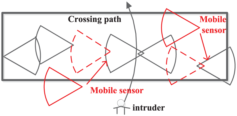
Repair the barrier gap by mobile sensors.

On one hand, when the stationary sensors in the target area cannot form a barrier, we need to redeploy the mobile sensors to improve the barrier coverage. Therefore, whether we need to deploy mobile sensors for a given stationary sensor network is one of the problems we need to solve, which is defined as critical condition for mobile deployment (CCMD) problem in this article. The critical condition may be affected by deployment parameters of the DSN, such as the deployment density, the sensing radius of each sensor, and the sensing angle of each sensor.

On the other hand, most sensors have limited power sources, and the batteries of the sensors are hard to replace due to the hostile or inaccessible environments in many scenarios. So, constructing energy-efficient barrier for DSNs is the other problem we need to solve, which is defined as energy-efficient barrier repair (EEBR) problem in this article. As shown in Figure 1, a barrier will be formed only when both mobile sensors are relocated to the desired locations. The moving distance significantly determines how long the target area can be barrier covered. Therefore, minimizing the maximum distance traveled by any sensor will balance the power consumption among sensors, which prolong the network lifetime.

In this article, we consider the following scenario. The target area is a two-dimensional (2D) Euclidean plane. A number of directional sensors are deployed uniformly and independently at random in the area following a Poisson point process. Our contributions are as follows:

We define and solve the CCMD problem. We divide the target area into squares of equal size and convert the barrier coverage problem to a bond percolation model. By our analysis, the CCMD depends on the deployment density ( $λ$ ) and the sensing radius (r). When the stationary network which deployed in the target area satisfies $λ > 8 \ln 2 / r^2$ , the target area can be barrier covered by the stationary network, and we do not need to redeploy mobile sensors. This result we obtained will provide important guidelines to the deployment and performance of DSN for barrier coverage.

We define and solve the EEBR problem. We propose an EEBR algorithm. First, we construct a flow graph based on the sensor location in formation. Then, we compute the maximum flow from the source node to the sink node of the flow graph. Each feasible flow in the flow graph can form a barrier for the sensor network. Finally, we choose the barrier which has the minimax moving distance to work for the sensor network. Through extensive simulations, the results show that the EEBR algorithm can improve the barrier coverage and prolong the network lifetime by minimizing the maximum sensor moving distance.

The rest of this article is organized as follows: In section “Related work,” we briefly survey the related work on barrier coverage of sensor network. In section “Network model and problem statement,” we describe the network model and define the CCMD and EEBR problems. In section “Solution to the CCMD problem,” we present and evaluate a solution to the CCMD problem. In section “Solution to the EEBR problem,” we propose an EEBR algorithm to solve the EEBR problem and give the simulation results of the algorithm. Finally, we conclude this article in section “Conclusion.”

Related work

In the past years, the barrier coverage problem in wireless sensor networks has been fairly well studied in the literature.

Most of the barrier coverage literatures assumed that every sensor node is stationary in the sensor networks. Zhang et al.³ presented several efficient centralized algorithms and a distributed algorithm to solve the strong barrier coverage problem for DSNs. The algorithms they proposed provided close-to-optimal solutions and consistently outperformed a simple greedy algorithm. Wang and Cao⁴ considered the problem of constructing camera barrier in both random and deterministic deployment. They proposed a novel method to select camera sensors to form a camera barrier, which is essentially a connected zone across the monitored field such that every point within this zone is full view covered. Chen et al.⁵ introduced the concept of local barrier coverage and proved that it is possible for individual sensors to locally determine the existence of local barrier coverage, even when the region of deployment is arbitrarily curved. They also developed a novel sleep–wake-up algorithm to maximize network lifetime. The algorithm they proposed outperformed randomized independent sleeping (RIS) algorithm by up to 6 times. Chen et al.⁶ believed quality of barrier coverage is not binary. They proposed a metric for measuring the quality of k-barrier coverage and established theorems that can be used to precisely measure the quality using the proposed metric. Stefan et al.⁷ studied three problems: the feasibility of barrier coverage, the problem of minimizing the largest relocation distance of a sensor (MinMax), and the problem of minimizing the sum of relocation distances of sensors (MinSum). Guo et al.⁸ studied the problem of constructing a β-breadth belt barrier with the minimum number of sensors thoroughly, both under 2D circumstances and three-dimensional (3D) circumstances. Besides, they extended this problem and studied how to build up k-disjoint β-breadth belt barriers under both 2D and 3D circumstances. Zhang et al.⁹ studied two problems: relocation of sensors with minimum number of mobile sensors and formation of k-barrier coverage with minimum energy cost. They relaxed the integrality and complicated constraints of the formulation and constructed a special model known as RELAX-RSMN with a totally unimodular constraint coefficient matrix to solve the relaxed 0-1 integer linear programming rapidly through linear programming. In Liu et al.,¹⁰ the authors first showed that in a rectangular area of width w and length l with $w = Ω (logl)$ , if the sensor density reached a certain value, then there existed, with high probability, multiple disjoint sensor barriers across the entire length of the area such that intruders cannot cross the area undetected. However, if $w = o (logl)$ , then with high probability, there was a crossing path not covered by any sensor regardless of the sensor density. Based on this result, they further proposed an efficient distributed algorithm which constructs multiple disjoint barriers in a large sensor network to cover a long boundary area of an irregular shape. Cheng and Wang¹¹ defined a new type of coverage problem named target-barrier coverage problem in wireless sensor networks. They focused on how to minimize the number of members required to construct target barriers in a distributed manner while satisfying the bound constraint and minimizing the amount of message exchange required. In Cheng and Wang,¹² they proposed algorithm that used mobile elements to check the presence of intruders at potential breach points. Compared with the extant algorithms, the proposed algorithm had two major advantages. First, it did not remove crossing barriers, so the overall network lifetime of barrier coverage could be extended. Second, it did not alternate working barriers always based on the order of barrier’s distance to the front side, from near to far, so the sleep–wake-up schedule could be flexibly arranged.

There are some literatures which focus on barrier coverage for sensor networks with mobile sensors. Saipulla et al.¹³ studied the barrier coverage with mobile sensors of limited mobility. They first explored the fundamental limits of sensor mobility on barrier coverage and presented a sensor mobility scheme that constructs the maximum number of barriers with minimum sensor moving distance. They further devised an algorithm that computed the existence of barrier coverage under the limited sensor mobility constraint and constructed a barrier if it exists. In He et al.,¹⁴ the authors considered the barrier coverage problem where n sensors are needed to guarantee full barrier coverage, and there are only m mobile sensors available (m < n). They first modeled the arrival of intruders at a specific location as a renew process. Then, they proposed two sensor patrolling algorithms to solve the problem: periodical monitoring scheduling (PMS) and coordinated sensor patrolling (CSP). In Keung et al.¹⁵ demonstrated the intrusion detection problem as a classical kinetic theory of gas molecules in physics. By examining the correlations and sensitivity from the system parameters, they derived the minimum number of mobile sensors that needs to be deployed in order to maintain the k-barrier coverage for a mobile sensor network. The algorithm proposed in Li and Shen¹⁶ computed a permutation of the left and right endpoints of the moving ranges of all the sensors forming a barrier coverage and minimized the maximum sensor movement distance by characterizing permutation switches that are critical. Tian et al.¹⁷ studied the barrier coverage problem in a mobile survivability heterogeneous wireless sensor network, which is composed of sensor nodes with environmental survivability to make them robust to environmental conditions and with motion capabilities to repair the barrier when sensors are dead. Shen et al.¹⁸ studied how to efficiently schedule mobile sensor nodes to form a barrier when sensor nodes suffer from location errors. They explored the relationship between the existence of uncovered hole and location errors and found that the lengths of uncovered holes are decided by the cumulative location errors. They also proposed a method in the frequency domain to efficiently calculate the distributions of the cumulative location errors. In Kim et al.,¹⁹ the authors first proposed a simple heuristic algorithm. Then, they designed another efficient algorithm for the problem and proved that the lifetime of hybrid barrier constructed by the algorithm is at least 3 times greater than the existing one on average.

Most of existing solutions to barrier coverage problem aim to find as many barrier sets as possible to enhance coverage for the target area. However, power conservation is still an important issue in DSNs and has not been carefully addressed in previous works.

Network model and problem statement

We assume that N directional sensors are deployed in a 2D rectangular region of length l and width w. In a realistic network scenario, the 2D rectangular region is usually referred to a strip. We assume that each sensor knows its coordinates of its own location. This may be done using an onboard Global Positioning System (GPS) or other localization mechanisms. Each sensor has a sensing range r and a sensing angle θ. Different from stationary sensors, mobile sensors can move after they are deployed. Existing mobile sensor platforms are often powered by small batteries which significantly limit the range of their movement. For instance, the onboard batteries of Robomote nodes only last for 20 min in full motion. Given a typical speed of 15 cm/s, the range of movement is only about 180 m. In this article, we assume that each mobile sensor has a uniform maximum moving range, which is denoted as R (R > 2r).

We adopt the widely used Boolean sensing model. The sensing region of a sensor is a sector of the sensing disk centered at the sensor with a sensing radius. Each sensor can rotate to different directions. We denote b_i,k as the kth direction of the ith sensor in the network. An intruder is said to be detected by a direction of a sensor if it lies within the direction’s sensing area. The sensing areas of different directions of a sensor do not overlap. Not more than one direction of the same sensor can work at the same time. A total of two directions of different sensors are said to be connected if their sensing areas overlap. A directional barrier is formed by a set of connected directions that intersects both of the left and right boundaries of the target area. We define it as follows:

Definition 1

A directional barrier is a subset of directions of the sensors such that (1) the leftmost and the rightmost directions overlap with the left and right boundaries of the target region, respectively; (2) any two neighboring directions overlap; and (3) it includes at most one direction from each sensor node.

Obviously, no intruders can cross such a directional barrier without being detected. Because of mechanical inaccuracy and other environmental factors, the sensors cannot be deployed as we desired. We cannot find a directional barrier for the network, as the barrier gaps may exist. We need to move the mobile sensor to improve the barrier coverage. When we need to deploy mobile sensor and how to construct an energy-efficient barrier with mobile sensors are the two problems we will solve in this work.

Definition 2

CCMD problem: Given a stationary DSN over the target area A, CCMD problem is to determine whether we need to deploy mobile sensors to improve the barrier coverage.

Definition 3

EEBR problem: When the DSN cannot form a barrier for the target area after the initial stationary deployment. EEBR problem is to construct an energy-efficient barrier for DSNs with mobile sensors such that the network lifetime is maximized.

Solution to the CCMD problem

In this section, we will solve the CCMD problem.

Deployment analysis for strong barrier

We consider the stationary sensor network scenario where sensors do not move after the initial deployment. We assume that the sensor locations follow a Poisson point process, where sensors are uniformly distributed in a 2D strip area of size A = [0, l] × [0, w]. We assume the density of the Poisson point is $λ$ . Thus, the expected number of nodes in the network is $λ lw$ .

Sensors have the equal likelihood to be located at any point in the rectangle. Thus, the sensors are spread out rather evenly in the area. By the widely adopted Boolean sensing model, the directional sensor can detect the target which is located in its sensing region. Thus, in DSNs, two sensors at locations $X_{i}$ and $X_{j}$ are connected if $‖ X_{i} - X_{j} ‖ \leq r$ , where $‖ X_{i} - X_{j} ‖$ is the distance between the two sensors. In DSNs, a barrier is formed by a set of connected sensors which intersects both of the left and right boundaries of the target area.

We convert the barrier coverage problem to a bond percolation model¹⁷ as follows: First, we divide the target area into squares of equal size, where the length of each side is $a = \sqrt{2} r / 4$ , as shown in the left-hand side of Figure 2. Then, we add Horizontal edges across half of the squares and vertical edges across others, as shown in the right-hand side of Figure 2. Thus, this construction results in a 2D lattice which consists of a grid of horizontal and vertical edges.

Figure 2.

Construction of the bond percolation model.

We consider the barrier coverage problem for a single square. As Figure 3(a) shows, if the sensor is located at the boundary of the square, it can form a barrier for this square by rotating its sensing directions. However, when the sensor is located in the square, it cannot form a barrier for the square in which it is located, which is shown in Figure 3(b).

Figure 3.

Barrier coverage for a single square: (a) sensor located at the boundary of the square and (b) sensor located in the square.

Then, we consider the barrier coverage for two adjacent squares. As Figure 4 shows, A₁ and A₂ are two adjacent squares. Sensors S₁ and S₂ are located in A₁ and A₂, respectively. The sensing radii of these two sensors are as same as r. On one hand, the distance between S₁ and the left boundary of A₁ is less than r, and therefore, S₁ can connect the left boundary of A₁. On the other hand, the length of the side is $\sqrt{2} r / 4$ . Therefore, the distance between S₁ and S₂ is less than or equal to r. S₂ can connect S₁. We can show that S₂ and S₁ can form a barrier for A₁.

Figure 4.

Barrier coverage for adjacent squares.

Considering the analyzed conclusion above, if both two adjacent squares have sensors, the left-hand side square can be barrier covered by the two sensors and no intruder can cross without detected. Therefore, if there is at least one sensor in each square, the target area could be barrier covered. Since stationary sensors deployed in a target area follow a Poisson point process with the density $λ$ and the sensing radius of the sensor r, we can obtain the probability of a square containing at least one sensor $p_{s}$ as follows

p_{s} = 1 - e^{- λ a^{2}}

(1)

A square is said to be open if it is occupied by at least one sensor and closed otherwise. If the squares along the path are all open, the path from left to right of the strip forms a barrier which can detect any intruder. A path consisting of a sequence of consecutive edges is open if every edge in the path is open. Therefore, the probability of a square containing at least one sensor ( $p_{s}$ ) is the same as the probability of every edge is open which is defined as $p_{e}$ .

As proposed in Grimmett,²⁰ the critical probability of $p_{e}$ is equal to 1/2; hence, we can obtain

p_{s} = 1 - e^{- λ a^{2}} = p_{e} > \frac{1}{2}

(2)

Therefore, the CCMD is

λ > \frac{8 \ln 2}{r^{2}}

(3)

When the deploy density $λ$ of the stationary network satisfies $λ > 8 \ln 2 / r^2$ , the percolation probability is greater than 0. In other words, there is at least one open path from the left to the right of the bond percolation model. We do not need to add mobile sensors to the network. The stationary sensors in this path can form a barrier for the target area detecting the intruder which wants to across the target area.

Analysis and simulation

We study the barrier coverage problem above by considering the directional sensor nodes distributed according to a Poisson point process. And we obtain the analysis result for the CCMD. Now, in this section, we compare our analysis described in section “Deployment analysis for strong barrier” and simulation results in different scenarios. We study the relationship between the barrier coverage probability and the network parameters, such as the deployment density ( $λ$ ), the sensing radius of each sensor (r), and the sensing angle of each sensor ( $θ$ ).

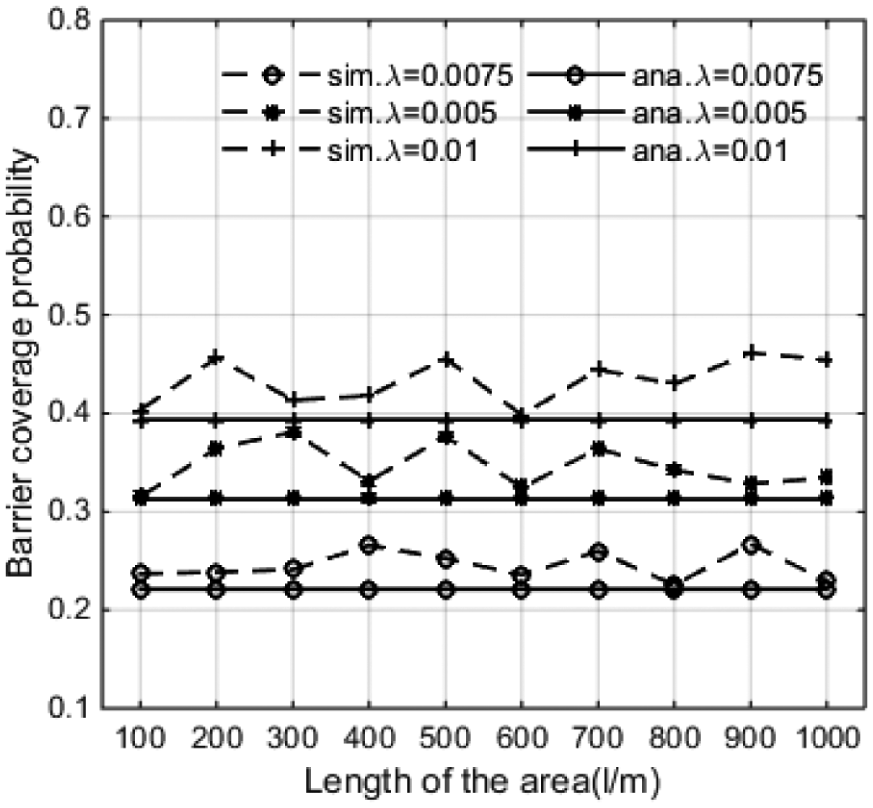
Figure 5 plots the relationship between the probability of barrier coverage and the length of the target area with the sensing radius of each sensor r = 20 m and the sensing angle of each sensor $θ = π / 2$ . Figure 6 plots the relationship between the probability of barrier coverage and the sensing radius of each sensor with the target area 1000 m × 500 m and the sensing angle of each sensor $θ = π / 2$ . In these two figures, we consider three different deployment densities $λ = 0.0075$ , $λ = 0.005$ , and $λ = 0.01$ . Figure 7 plots the probability of barrier coverage when the sensing angles of each sensor are $2 π / 3$ , $π / 2$ , $π / 3$ , and $π / 6$ . In Figure 7, the sensing radius of each sensor is r = 40 m, and the deployment density is $λ = 0.0075$ .

Figure 5.

Probability of barrier coverage for various area lengths for the Poisson deployment.

Figure 6.

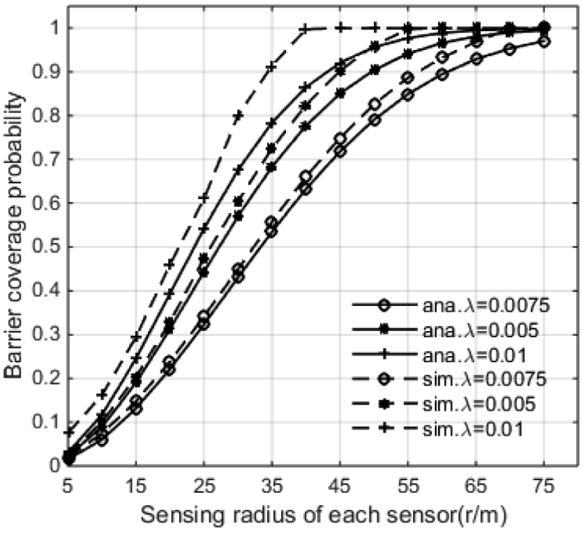
Probability of barrier coverage for various sensing radii for the Poisson deployment.

Figure 7.

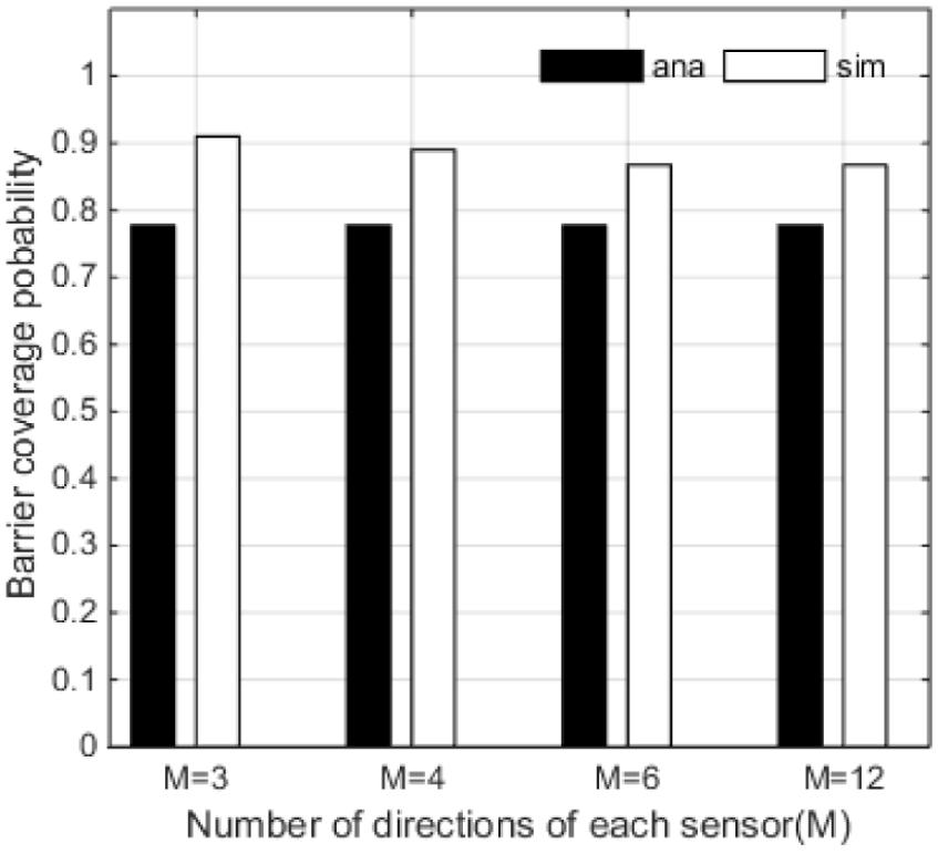
Probability of barrier coverage for various sensing angles for the Poisson deployment.

In Figure 5, we can see that the length of area l is varied from 100 to 1000 m. Because the number of sensors which are deployed in the area is $N = λ lw$ . When the length of area increases, the number of sensors increases, which guarantees the barrier coverage probability for the target area. In Figure 6, we can see that the probability of barrier coverage increases monotonically as the sensing radius of each sensor increases. The reason is that when the sensing radius increases, the number of sensors we need to form a barrier decreases. Therefore, the network has more probability to form a barrier for the area. Figure 7 implies that the sensing angle of each sensor has no effect on the probability both in our analysis and simulation results.

We can observe from the results above that there is a good match between our analysis and simulation. Also, we verify that our analysis is indeed a lower bound than the simulation. The CCMD in a stationary sensor network is sensitive to the deployment density and the sensing radius. When it satisfies $λ < 8 \ln 2 / r^2$ , we need to deploy mobile sensors in the target area to improve barrier coverage. Our analysis can guide the deployment methods and parameters in the realistic application.

Solution to the EEBR problem

In this section, we mainly consider the energy consumption of sensor movement. To prolong the lifetime of the network, the maximum moving distance of mobile sensors should be minimized.

Barrier gap

In stationary networks, if the number of deployed sensors is not large enough, barrier gaps may exist. In this section, we will focus on how to repair barrier gaps. First, we need to find the barrier gaps in the stationary sensor networks.

Definition 4

Barrier gap: When the sensing directions b_i,p and b_j,q satisfy the three conditions, there is a barrier gap between b_i,p and b_j,q, which is denoted by (b_i,p, b_j,q):

b_i,p and b_j,q belong to different sensors;

b_i,p cannot connect with b_j,q;

b_i,p and b_j,q are two adjacent nodes.

The barrier gap is that area which is not covered by any sensor, and the intruder can cross without detected. Whether the barrier gap can be repaired is determined by two aspects: (1) the repair location for the barrier gap and (2) the distance between the mobile sensor and the repair location.

Given a directional sensor with sensing radius r and sensing angle θ. The maximum region the sensor can sense is L

L = {\begin{matrix} r, 0 < θ \leq \frac{π}{3} \\ r \sin (\frac{θ}{2}), \frac{π}{3} < θ < 2 π \end{matrix}

(4)

For simplicity, we only consider the barrier gap which one sensor can repair. Therefore, the shortest distance between b_i,p and b_j,q which is denoted by d_ij is less than L. We consider the following cases: case 1 and case 2, to find the repair location for the gap (b_i,p, b_j,q). The line segment D₁D₂ is the shortest distance between b_i,p and b_j,q. The point O is the midpoint of D₁D₂.

Case 1: d_ij≤r. As Figure 8(a) shows, the points D₁ and D₂ are in the sensing region of the directions b_i,p and b_j,q, respectively. The line segment D₁D₂ satisfies ||D₁D₂|| = d_ij. In other words, the length of D₁D₂ is less than r. In this case, the maximum sensing range of a mobile sensor is r. So, when the mobile sensor moves to D₁ or D₂, it can intersect with b_i,p and b_j,q. Therefore, in this case, the repair location of gap (b_i,p, b_j,q) is D₁ or D₂.

Case 2: r < d_ij < L. As Figure 8(b) shows, the points D₁ and D₂ are in the sensing region of the directions b_i,p and b_j,q, respectively. The line segment D₁D₂ satisfies ||D₁D₂|| = d_ij. In other words, the length of D₁D₂ is greater than r. When the mobile sensor moves to D₁ or D₂, it cannot intersect with b_i,p and b_j,q. So, D₁ and D₂ cannot be the repair location for the gap (b_i,p, b_j,q). We draw a perpendicular bisector h of line segment D₁D₂. The point O is the intersect point of h and D₁D₂. We identify two points D₃ and D₄ on h, which satisfy ||D₃D₄|| = rcos(θ/2). In this case, the maximum sensing region of a mobile sensor is L, which satisfies L > ||D₃D₄||. So, when the mobile sensor moves to D₃ or D₄, it can intersect with b_i,p and b_j,q. Therefore, in this case, the repair location of gap (b_i,p, b_j,q) is D₃ or D₄.

Figure 8.

Repair location for the barrier gap: (a) when d_ij≤r and (b) when r < d_ij < L.

Then, the mobile sensor around the gap can repair the barrier gap if the distance between its location and repair location is less than R. The energy of mobile sensor which is consumed by repairing the barrier gap mainly depends on the moving distance. To prolong the lifetime, we need to choose the mobile sensor which has the minimum moving distance to repair the gap.

Constructing an energy-efficient barrier

In this section, we present an EEBR algorithm for DSNs with mobile sensors. We assume that the location of each sensor is collected prior to computation. We first construct a graph based on the sensor location information as follows:

We model a directed graph G(V, E) for the sensors in the network. Vertex $v_{i} (v_{i} \in V)$ represents directions of each sensor. There is a directed edge between $v_{i} (v_{i} \in V)$ and $v_{j} (v_{j} \in V)$ , if $v_{i}$ and $v_{j}$ overlap and they belong to different sensors.

From G(V, E), construct a flow graph $G^{*} (V^{*}, E^{*}, C)$ as follows: $\forall v_{i} \in V$ , add $v_{i}$ to $V^{*}$ , and $\forall (v_{i}, v_{j}) \in E$ , add ( $v_{i}, v_{j}$ ) to $E^{*}$ . Add a virtual source node $v_{0}$ to $V^{*}$ , and if the direction which $v_{i} (v_{i} \in V)$ is corresponding to covers the left boundary, add ( $v_{0}, v_{i}$ ) to $E^{*}$ , add a virtual sink node $v_{t}$ to $V^{*}$ , and if the direction which $v_{i} (v_{i} \in V)$ is corresponding to covers the right boundary, add ( $v_{i}, v_{t}$ ) to $E^{*}$ . If there is a barrier gap which is defined in section “Barrier gap” between $v_{i} (v_{i} \in V)$ and $v_{j} (v_{j} \in V)$ , and the mobile sensor $v_{k} (v_{k} \in V)$ can repair the gap, add ( $v_{i}, v_{k}$ ) and ( $v_{k}, v_{j}$ ) to $E^{*}$ . Set capacity ( $v_{i}, v_{j}$ ) = 1 if $(v_{i}, v_{j}) \in E^{*}$ .

Obviously, each feasible flow from $v_{0}$ to $v_{t}$ of $G^{*} (V^{*}, E^{*}, C)$ containing different static nodes and mobile sensors can form a directional barrier for the sensor network. Therefore, we can obtain all the possible barriers for the sensor network by the maximum flow algorithm. We use Ford–Fulkerson algorithm²¹ to compute and return the maximum flow from $v_{0}$ to $v_{t}$ in $G^{*} (V^{*}, E^{*}, C)$ , which is defined as $Maxflow (G^{*})$ . Each flow $f (f \in Maxflow (G^{*}))$ is a possible barrier for the sensor network. We compute the maximum moving distance for each barrier. Then, the barrier with the minimax moving distance will be chosen to work for the target area.

The following EEBR algorithm tests whether there exists a barrier across the target area and finds an energy-efficient barrier by considering the minimax moving distance.

Algorithm 1. EEBR algorithm.
1. Construct a directed graph G = (V, E) 2. if (there is a path from $v_{0}$ to $v_{t}$ in G) 3. return the path and d = 0; 4. else 5. Construct a flow graph $G^{} (V^{}, E^{}, C)$ 6. Use Ford–Fulkerson algorithm to compute the maximum flow $Maxflow (G^{})$ in $G^{}$ 7. for each flow $f (f \in Maxflow (G^{}))$ 8. Compute maximum moving distance D 9. ifD < d 10. d = D, f′ = f 11. endif 12. end 13. returnd, f′ 14. endif

Algorithm 1. EEBR algorithm.

1. Construct a directed graph G = (V, E)
2. if (there is a path from

v_{0}

v_{t}

in G)
3. return the path and d = 0;
4. else
5. Construct a flow graph

G^{*} (V^{*}, E^{*}, C)

6. Use Ford–Fulkerson algorithm to compute the maximum flow

Maxflow (G^{*})

G^{*}

7. for each flow

f (f \in Maxflow (G^{*}))

8. Compute maximum moving distance D
9. ifD < d
10. d = D, f′ = f
11. endif
12. end
13. returnd, f′
14. endif

When the EEBR algorithm terminates, it will return to the barrier and the minimax moving distance. The target area can be barrier covered by the barrier with the maximum network lifetime. Finding maximum flow from $v_{0}$ to $v_{t}$ in $G^{*}$ terminates in $O (V^{*} {E^{*}}^{2})$ iterations. Computing minimax moving distance terminates in O(m²). So, the total running time of EEBR algorithm is $O (V^{*} {E^{*}}^{2} + m^{2})$ .

Simulation results

In this section, we present the performance of the EEBR algorithm and compare it with the energy-efficient barrier coverage (EEBC) algorithm.²² In the simulation, we assume that our algorithm is computed in the sink node. Before the network starts to monitor the target area, the information of the barrier set is broadcasted to each sensor node. For simplicity, we assume that the initial lifetime of each sensor is unit 1.

Barrier coverage probability

Figure 9 shows the effect of the fraction of the mobile sensors on the probability of barrier coverage. In Figure 9, sensors are initially deployed uniformly at random in the target area of size 1000 m × 100 m. The sensing radius of each sensor is 10 m, and the sensing angle of each sensor is $π / 2$ . The maximum moving range of mobile sensor is set to be 30 m. We consider five different fractions of mobile sensors, 10%, 15%, 20%, 30%, and 40%. Figure 10 shows the effect of maximum sensor moving range on the probability of barrier coverage. In Figure 10, 300 nodes are deployed uniformly at random in target area of size 1000 m × 100 m. The fraction of mobile sensors is 15%. The sensing angle of each sensor is $π / 2$ . We consider five different maximum moving ranges of mobile sensors, 20, 30, 40, 50, and 60 m.

Figure 9.

Probability of barrier coverage versus fraction of mobile sensors (EEBR vs EEBC).

Figure 10.

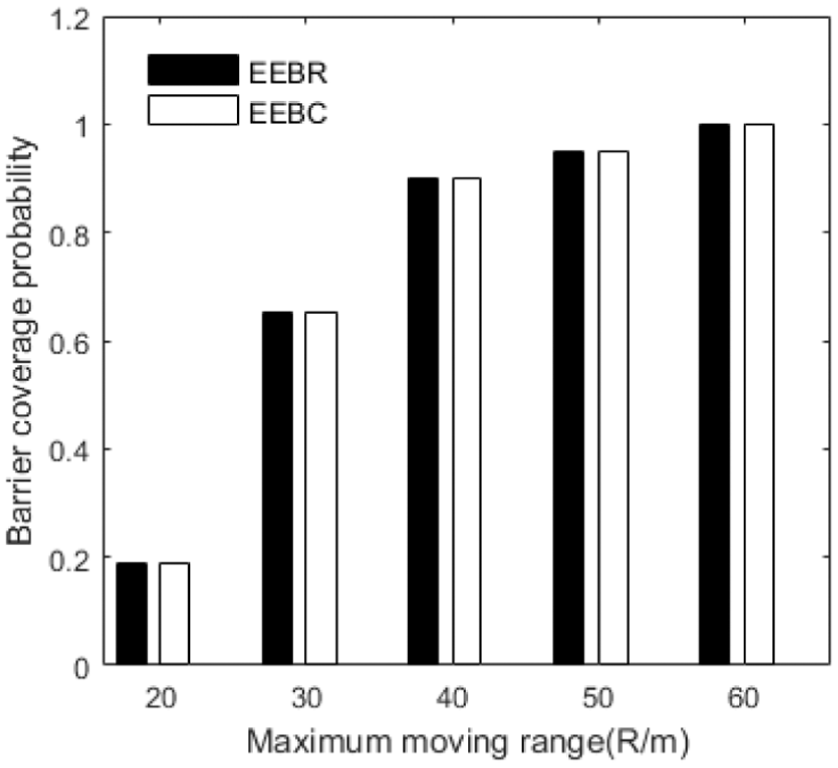
Probability of barrier coverage versus maximum moving range (EEBR vs EEBC).

In Figure 9, we can observe that as we increase the fraction of mobile sensors, the probability of successfully forming a barrier starts rising up rapidly and eventually levels off to 1. This result is important for network deployments, as it shows that increasing the fraction of mobile sensors leads to significant improvement in barrier coverage. As shown in Figure 10, when the maximum moving range increases, sensors can move farther, and more barriers can be formed, resulting in a rapid increase of the barrier coverage probability. This result shows that for a fixed fraction of mobile sensors, the setting with the larger maximum moving range always yields higher probability of barrier coverage. In Figures 9 and 10, we can also observe that barrier coverage probability of the EEBR algorithm is always the same as that of the EEBC algorithm. EEBC algorithm first finds all the possible barriers and then chooses the one which has the minimum gaps. EEBR algorithm first finds all the possible barriers and then chooses the one which has the minimum maximum moving distance. Therefore, both EEBR algorithm and EEBC algorithm can find all the possible barriers for the DSN. In other words, barrier coverage probability is the same for EEBR and EEBC in all cases.

Network lifetime

Figure 11 shows the effect of sensing radius on the network lifetime. In Figure 11, the size of the target area is 1000 m × 500 m. The total number of sensors varies from 0 to 600, and the fraction of mobile sensors is 15%. The maximum moving range is set to be 30 m. We consider three different sensing radii of each sensor, which are set to 10, 30, and 50 m, respectively. Figure 12 shows the effect of the maximum moving range on the network lifetime. In Figure 12, 300 sensors are deployed uniformly at random in three different rectangle settings, 1200 m × 100 m, 800 m × 100 m, and 500 m × 100 m. The fraction of mobile sensors is 15%. Every sensor has a sensing radius of 10 m. The maximum moving range varies from 0 to 120 m.

Figure 11.

Network lifetime versus total number of sensors (EEBR vs EEBC).

Figure 12.

Network lifetime versus maximum moving range (EEBR vs EEBC).

As shown in Figure 11, for each curve, when the total number of sensors increases, the network lifetime quickly increases to 1. We can also observe that as the sensing radius increases, the moving distance decreases, which could save the energy consumption. This result shows that the network lifetime increases as more redundant sensors are added. And we can prolong the network lifetime by adding the sensing radius of each sensor. In Figure 12, as the length of the target area increases, the network lifetime decreases. We can observe that for each curve, there is a transition point where the network lifetime does not add at all. This result shows that for a network scenario, when the barrier coverage probability is close to 1, adding maximum moving range of each mobile sensor cannot prolong the network lifetime.

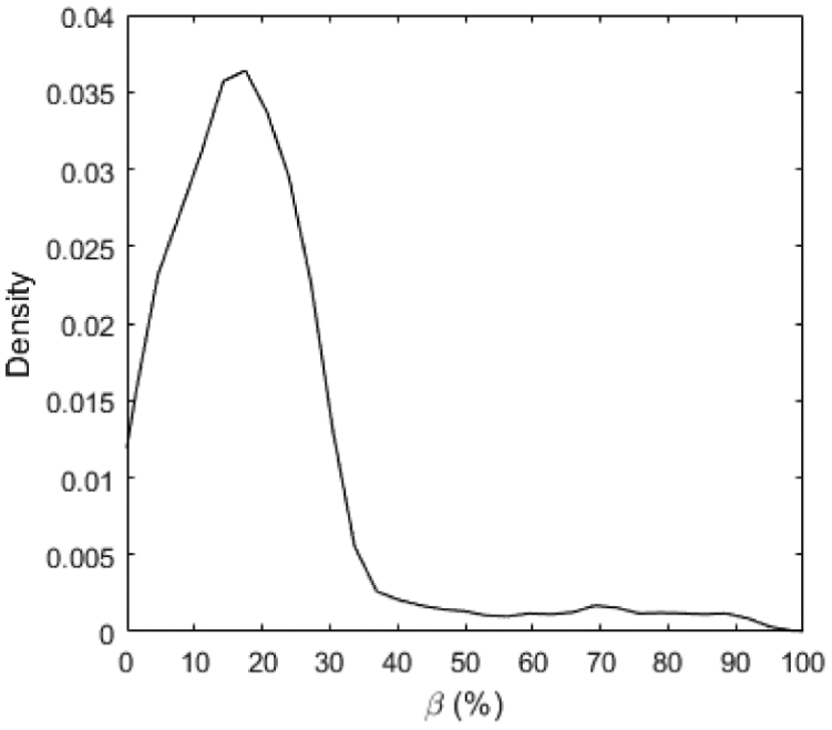
It can be seen from Figures 11 and 12 that the EEBR algorithm yields much more network lifetime in comparison with the EEBC algorithm. Figure 13 shows what percentage of network lifetime the EEBR algorithm can improve. We denote $β$ as the percent which the EEBR algorithm increased compared with the EEBC algorithm, $β = ((T_{EEBR} - T_{EEBC}) / T_{EEBC}) * 100 %$ . $T_{EEBR}$ is denoted as the network lifetime of EEBR algorithm. $T_{EEBc}$ is denoted as the network lifetime of EEBC algorithm. We randomly generate multiple deployments of directional sensors and plot the probability density function of $β$ , which is shown in Figure 13. We can see that the minimum value of $β$ is 0. It means that in some cases, the network lifetime is the same for EEBR and EEBC. In most cases, the value of $β$ is between 10% and 30%. And we can calculate that the average value of $β$ is 18%. This means that the EEBR algorithm can increase by 18% of network lifetime on average compared with the EEBC algorithm.

Figure 13.

Density distribution for $β$ .

Conclusion

In this article, we study the strong barrier coverage for DSNs with mobile sensors. We consider the following scenario. The target area is a 2D Euclidean plane. A number of directional sensors are deployed uniformly and independently at random in the area following a Poisson point process. We describe the network model and define CCMD and EEBR problems we need to solve. First, we derive CCMD, which depends on the deployment density and the sensing radius. The result we obtained will provide important guidelines to the deployment and performance of DSN for barrier coverage. Then, we propose an EEBR algorithm to construct a barrier for the DSN with mobile sensors. We first construct a flow graph based on the sensor location in formation and then compute the maximum flow of the flow graph. Each augmenting path forms a barrier in the sensor network. Through extensive simulations, we demonstrate that our algorithm has a desired barrier coverage performance for DSNs.

Footnotes

Handling Editor: Hassan Mathkour

Declaration of conflicting interests

The author(s) declared no potential conflicts of interest with respect to the research, authorship, and/or publication of this article.

Funding

The author(s) disclosed receipt of the following financial support for the research, authorship, and/or publication of this article: This work was supported by the National Natural Science Foundation of China under Grant Nos. 61502230 and 61073197, the Natural Science Foundation of Jiangsu Province under Grant No. BK20150960, and the Natural Science Foundation of the Jiangsu Higher Education Institutions of China under Grant No. 15KJB520015.

References

Balister

Bollobás

Sarkar

. Barrier coverage. Random Struct Algor 2016; 49(3): 429–478.

Tao

. A survey on barrier coverage problem in directional sensor networks. IEEE Sens J 2015; 15(2): 876–885.

Zhang

Tang

Zhang

. Strong coverage with directional sensors. In: Proceedings of the IEEE GLOBECOM global telecommunications conference, Honolulu, HI, 30 November–4 December 2009, pp.1816–1821. New York: IEEE.

Wang

Cao

. Barrier coverage in camera sensor networks. In: Proceedings of the 12th ACM international symposium on mobile ad hoc networking and computing (Mobihoc ‘11), Paris, 17–19 May 2011. New York: ACM.

Chen

Kumar

Lai

. Designing localized algorithms for Barrier coverage. In: Proceedings of the ACM Mobicom, Montreal, QC, Canada, 9–14 September 2007, pp.63–74. New York: ACM.

Chen

Lai

Xuan

. Measuring and guaranteeing quality of barrier coverage for general belts with wireless sensors. ACM Trans Sens Netw 2009; 6(1): 2.

Stefan

Stephane

Mohsen

et al . Complexity of barrier coverage with relocatable sensors in the plane. Theor Comput Sci 2015; 579(C): 64–73.

Guo

Zhu

et al . Enhancing barrier coverage with quality of monitoring in wireless camera sensor networks. Ad Hoc Netw 2016; 51(C): 62–79.

Zhang

Sun

Wang

. Efficient algorithm for k-barrier coverage based on integer linear programming. China Commun 2016; 13(7): 16–23.

10.

Liu

Dousse

Wangand

et al . Strong barrier coverage of wireless sensor networks. In: Proceedings of the 9th ACM international symposium on mobile ad hoc networking and computing (Mobihoc 08), Hong Kong, China, 26–30 May 2008, pp.411–419. New York: ACM.

11.

Cheng

Wang

. The target-barrier coverage problem in wireless sensor networks. IEEE T Mobile Comput. Epub ahead of print 11 September 2017. DOI: 10.1109/TMC.2017.2751040.

12.

Cheng

Wang

. The barrier-breach problem of barrier coverage in wireless sensor networks. IEEE Commun Lett 2017; 21(10): 2262–2265.

13.

Saipulla

Liu

Xing

et al . Barrier coverage with sensors of limited mobility. In: Proceedings of the 11th ACM international symposium on mobile ad hoc networking and computing (Mobihoc ‘10), Chicago, IL, 20–24 September 2010, pp.201–210. New York: IEEE.

14.

Chen

et al . Cost-effective barrier coverage by mobile sensor networks. In: Proceedings of the IEEE INFOCOM, Orlando, FL, 25–30 March 2012, pp.819–827. New York: IEEE.

15.

Keung

Zhang

. The intrusion detection in mobile sensor network. IEEE: ACM T Netw 2012; 20(4): 11–20.

16.

Shen

. Minimizing the maximum sensor movement for barrier coverage in the plane. In: Proceedings of the IEEE conference on computer communications, Kowloon, Hong Kong, 26 April–1 May 2015, pp.244–252. New York: IEEE.

17.

Tian

Liang

Wang

. Deployment and reallocation in mobile survivability-heterogeneous wireless sensor networks for barrier coverage. Ad Hoc Netw 2016; 36(1): 321–331.

18.

Shen

Weng

Wang

. Fault tolerant line-based barrier coverage formation in mobile wireless sensor networks. Int J Distrib Sens Netw 2015; 2015: 11.

19.

Kim

Wang

Son

et al . Maximum lifetime combined barrier-coverage of weak static sensors and strong mobile sensors. IEEE T Mobile Comput 2017; 16(7): 1956–1966.

20.

Grimmett

. Percolation. 2nd ed. Berlin: Springer, 1999.

21.

Lawler

. Combinatorial optimization: networks and matroids. New York: Renehart & Winston Press, 1977.

22.

Zhao

Bai

Shen

et al . Energy efficient barrier coverage in hybrid directional sensor networks. In: Proceedings of the international conference on wireless communications & signal processing (WCSP), Nanjing, China, 15–17 October 2015. New York: IEEE.